
Fitting Terrestrial Laser Scanner Point Clouds with T-Splines: Local Refinement Strategy for Rigid Body Motion


Abstract
:
1. Introduction
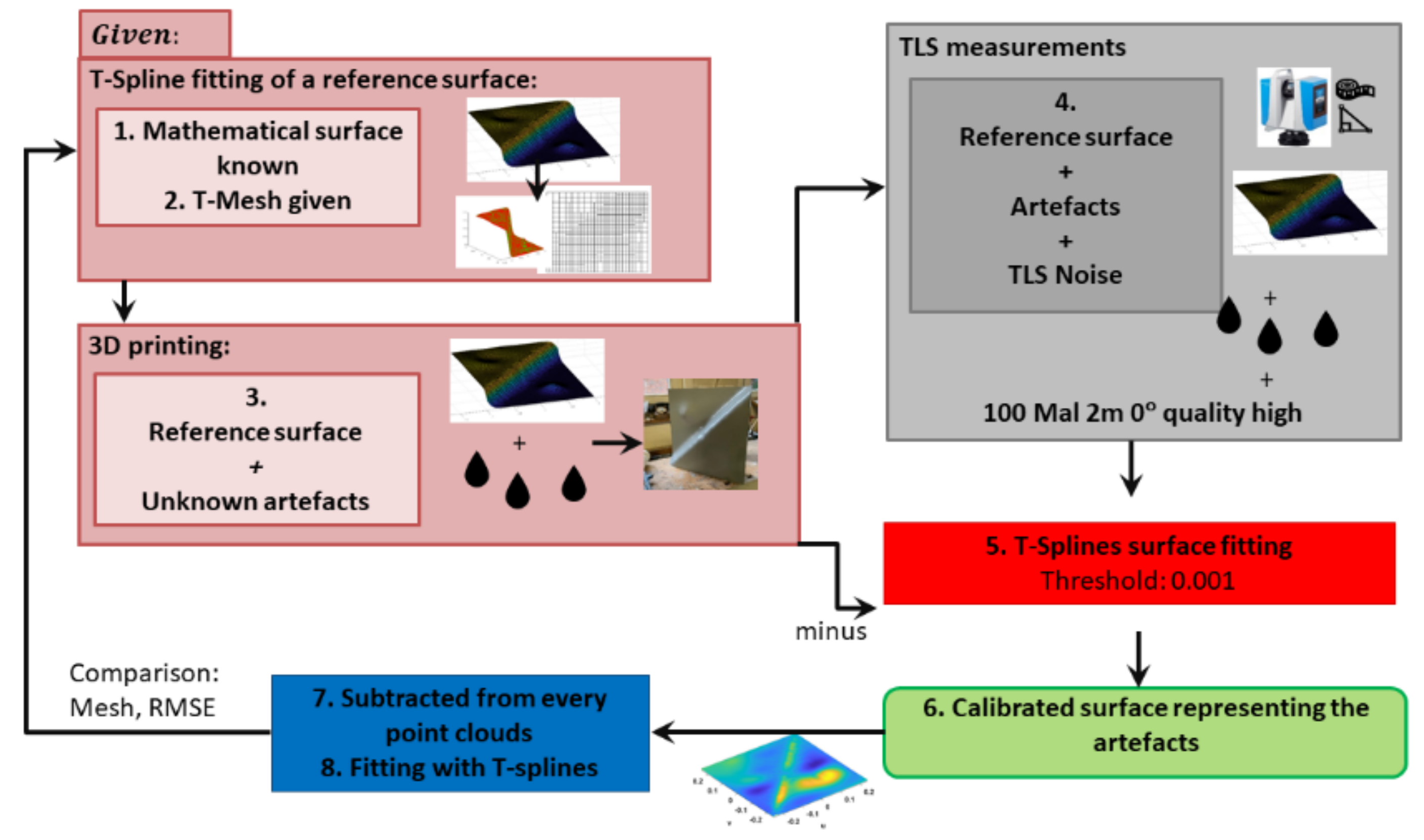
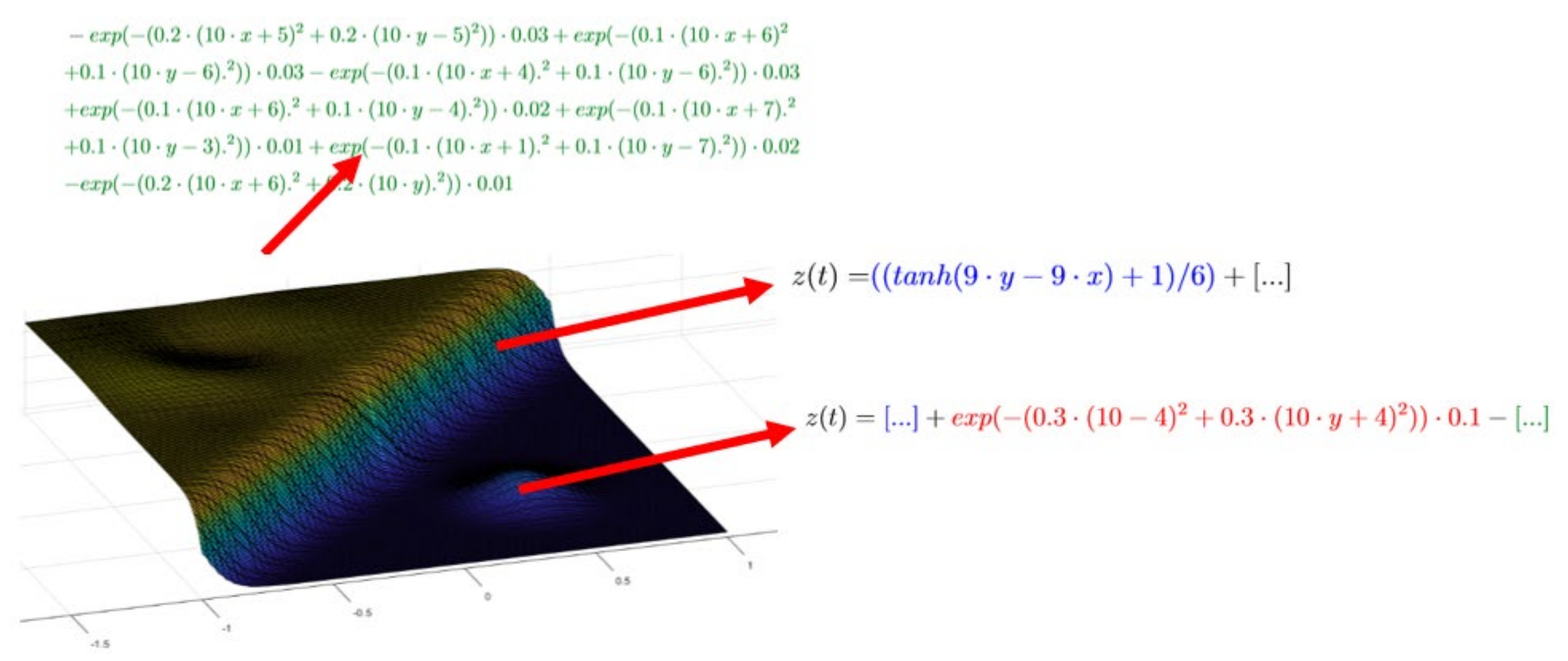
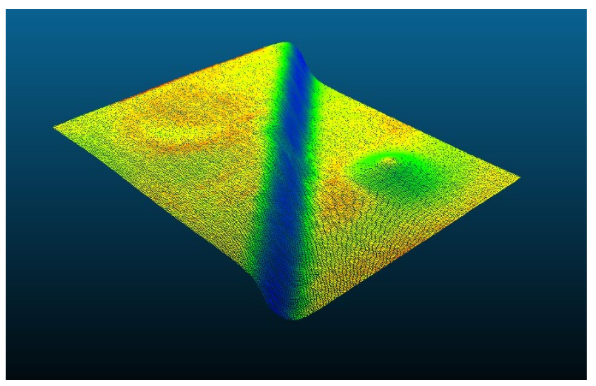
- Assessing the goodness of fit of surface approximation with T-splines. Accordingly, we use the high potential of three-dimensional (3D) printing. To that aim, we created and scanned with a TLS a 3D corpus corresponding to a known T-splines reference surface. Having modeled the inaccuracies due to the printing with Monte Carlo measurements, we allow a unique comparison between the known T-splines reference surface and the approximated noisy and scattered point cloud.
- Comparing the results of the adaptive fitting with the traditional but less locally flexible NURBS by highlighting the risky overfitting, i.e., fitting of the noise.
- Proposing a strategy in the case of the rigid body motion of an object to save computational time. Under rigid body motion, we understand that the shape of the body does not change strongly, only its orientation/distance in space: no strong strain or distortion occurs. We will investigate how to avoid repeating an iterative refinement for the second epoch of observations based on the mesh computed for the first epoch. This procedure can greatly simplify the analysis of deformation based on parametric surfaces and its rigorous statistical testing by significantly decreasing the computational time [27].
2. Surface Fitting Using T-Splines
2.1. Basis Concepts
2.2. Refinement Strategy
2.3. Iterative T-Spline Surface Approximation Using Least Squares
2.4. Criterion to Judge the Goodness of Fit
- The RMSE regarding the points to be approximated and also called average distance . Alternatively, an a posteriori variance factor could be computed, i.e., , as the mean of the error term computed with LS is 0. Since in this contribution , we will use the average distance RMSE, which has similarities to the average distance, as used in [26].
- The maximal error, .
- The number of points outside the tolerance , i.e., for which once the maximum of iterations allowed is reached. Note that the refinement is performed only if at least three points are outside the tolerance in this contribution. Consequently, even if the refinement stops, some cells may contain one or two points outside the tolerance. This strategy was chosen to avoid unnecessary cell refinement linked with the computational burden, when the observations may contain outliers.
3. From the 3D Printing of the Reference Surface to Its Scanning and Fitting
3.1. Mathematical Surface
3.2. 3D Printing
3.2.1. Principle
3.2.2. Preprocessing
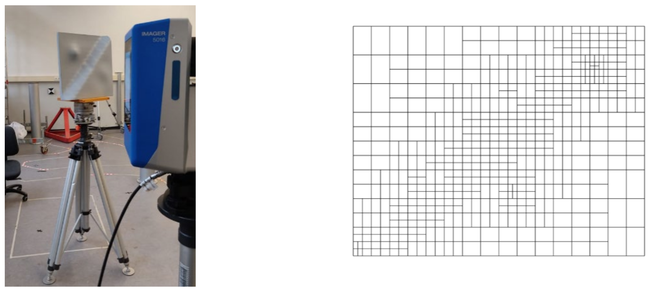
3.3. TLS Measurements
3.4. Calibration of the Printed Surface
- There is no error after the calibration compared to the 41 before calibration. This result confirms the presence of artefacts on the printed surface that were approximated by the iterative algorithm before calibration, leading to cells that still contain one or two errors.
- The Monte Carlo measurements permit the generation of a highly accurate calibrated surface: the point cloud approximated after the subtraction of the “droplets surface” became close to the printed reference; the RMSE reached 3.2 × 10⁻² mm, which corresponds to a decrease of 40% w.r.t. the RMSE before calibration. This small value after calibration highlights the high trustworthiness of the approximation, i.e., the closeness to the mathematical surface.
- The T-mesh is similar to the reference one, up to four points that were added supplementarily.
4. Approximation: Impact of the Scanning Configuration
- The approximation with T-splines and NURBS after calibration of the surface;
- The extent to which the original T-mesh can be reused for various configurations to avoid repeating the adaptive refinement and save computational time.
4.1. T-Splines Approximation by Varying the Scanning Configuration
4.1.1. Varying the Distance
- The RMSE for the reference surface increases by a factor between 1.2 and 1.5 approximately between the distances 4–2 and 6–4 m. This result seems strongly plausible as the number of scanned points decreases with the scanning distance. The number of points is about 140,000 for the distance of 2 m, 36,000 for 4 m and 18,000 for 6 m.
- There are no points outside tolerance except for the challenging tilting of 60° for which the number of errors reaches 25. This value is small compared with the size of the point clouds.
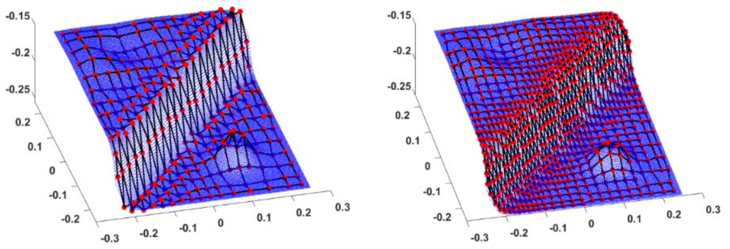
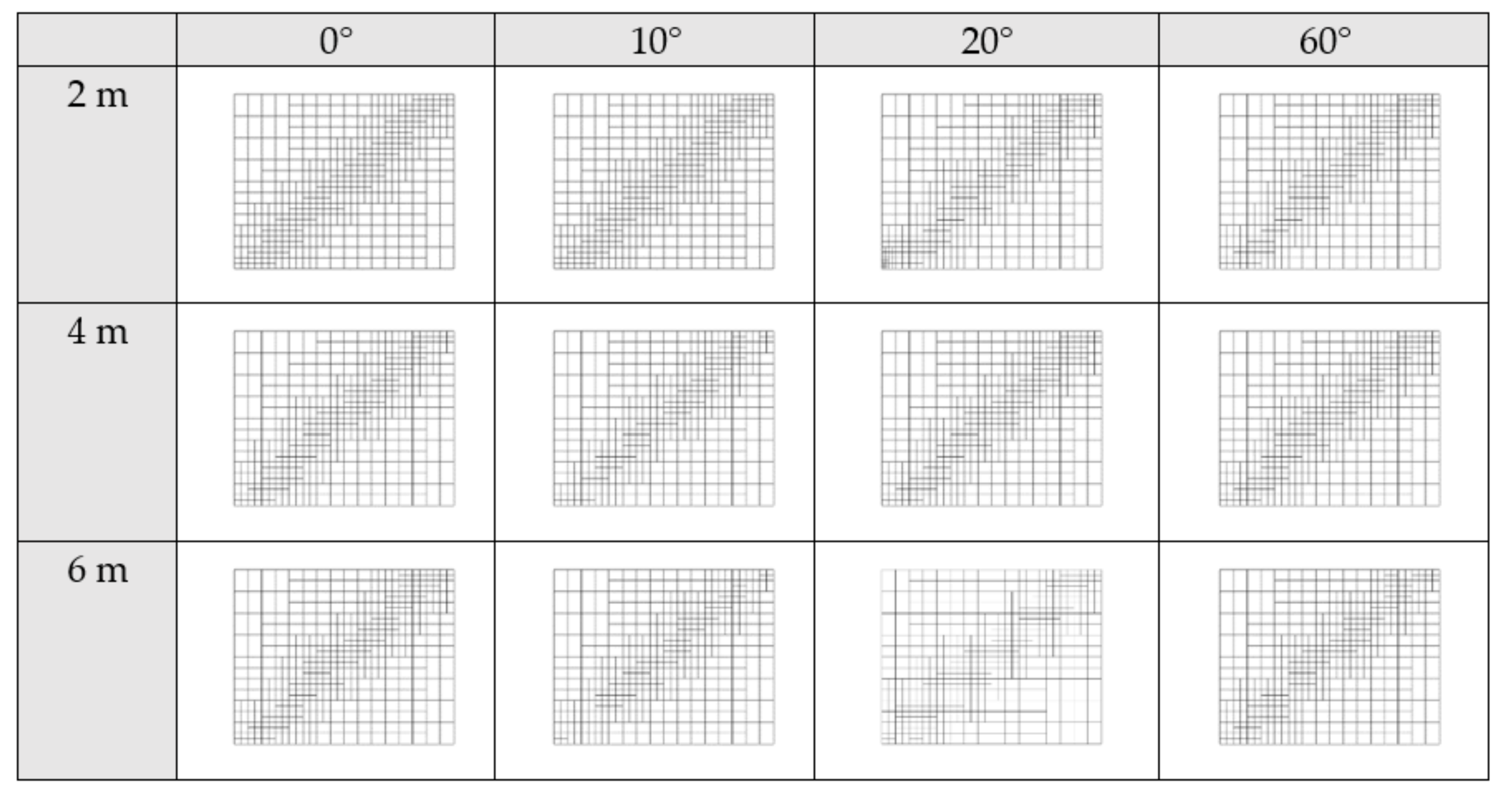
- The number of control points decreases slightly as the number of points to approximate becomes smaller, which is highlighted in Figure 10 with the corresponding T-meshes.
4.1.2. Varying the Tilting
- Leads to an approximative increase in the RMSE by a factor 2 between 0° and 60°. The maximum error becomes higher by up to a factor 3 for the distance of 2 m.
- Affects the repartition of the control points along the diagonal, i.e., along the dam. There are slightly less control points at the edges than for the reference T-mesh. This effect is linked with the repartition of the scanned points in space. This result has to be weighted by the very small value of the RMSE, making the differences statistically nearly insignificant.
- Does not lead to a strong variation in the number of control points to estimate. A maximum difference of 20 is observed due to the decrease in the number of scanned points, or the inclusion of lines in the T-mesh by the refinement algorithm caused by challenging geometries. Once more, the difference cannot be considered as significant and is not synonymous with a higher computational time.
- Increases the number of iterations needed to reach the tolerance. This effect is due to data gaps, shadowing effects or systematic errors, which necessitates a higher refinement level to reach the tolerance.
4.1.3. Further Comments and Conclusion
4.2. Comparison with NURBS
4.3. Avoiding Adaptive Refinement in Case of Rigid Body Motion
- Would be validated if the RMSE or the number of points outside tolerance does not change drastically between the reference and the T-mesh as used in Section 4.1 (Figure 10) to approximate the point clouds.
- Would avoid the re-computation of the basis functions and save computational time drastically when the same object is scanned at different epochs but only its orientation in space changes: no adaptive refinement would have to be performed for the second point cloud, and the approximation could be directly computed.
- Makes use of the property of a T-mesh: the T-mesh acts as a filter so that additional effects (systematic or stochastic information arising, e.g., when varying the tilting) could be eliminated.
4.4. Concluding Remarks
- We can be highly confident about the goodness of fit of a T-spline surface to a point cloud from a smooth surface.
- When the point clouds are rigidly deformed, an approximated mesh can be used with high confidence and a low impact on the RMSE for the reference, as only 1% of the points were outside the tolerance.
- Compared with the global refinement performed with NURBS, the main advantage of the local refinement strategy is to approximate the point cloud with a high definition only in some specific domains. Global refinement with NURBS may lead to an overfitting as the number of iterations increases. It is further linked with a strong increase in the computational time as the number of parameters to estimate increases. Local and adaptive refinement strategies should be preferred in the case of noisy and scattered point clouds.
5. Application: A Bridge under Load
5.1. Short Description of the Dataset
- approximate the two patches with T-splines;
- compare the T-meshes;
- perform the approximation for epoch E55 on the same T-mesh as epoch E00, i.e., without iteration. This will allow us to judge the feasibility of our methodology in the case of rigid body motion.
5.2. Results of the T-Splines Approximation and Comparison with NURBS
- The residuals do not show a spurious pattern, are nearly white and are below the millimeter level in norm. We note further that the number of errors is small regarding the size of the point clouds (170,000 points). Both remarks confirm the goodness of the approximation for the threshold chosen.
- The number of control points and errors was similar for both surfaces, which has to be linked with the fact that the patch did not change in shape but only in orientation.
- The maximum error may seem large: it fortunately concerns only a few points as the small RMSE of 1 mm indicates.
- The RMSE is similar to that for the NURBS approximation. The difference is approximately 0.1 mm for E00 (similar for E55 but not shown for the sake of shortness) and cannot be considered as significant. We insist that an RMSE that is too small is not synonymous with a good approximation, as the noise may have been fitted, as illustrated in the previous section. A good balance has to be found, by avoiding oscillations in the residuals. The residuals can be visually detected by inspecting the fitted surface.
- The number of control points to estimate for NURBS is three times higher than for T-splines for the same RMSE. This drawback increases the computational time by a factor 6 from 45 to 300 s. The corresponding NURBS mesh is shown in Figure 14 (bottom). Compared with the T-meshes of the two epochs (Figure 14, top), a lot more control points need to be introduced: 3550 versus 1141.
- The number of errors for NURBS increases with respect to the T-spline approximation due to the global refinement since all the cells of the mesh are halved, which corresponds to an extremely small threshold in an adaptive scheme.
5.3. “Re” Using the T-Mesh for Deformation Analysis
5.4. Summary
- Reduce the computational time regarding a global surface fitting using NURBS. The adaptive local refinement strongly decreases the number of parameters to estimate for the same order of the RMSE.
- Simplify the computation of the control points of the second epoch by using the same mesh as for the first epoch. This was made possible since the deformation of the patch was rigid, i.e., only its orientation changed and its shape was not strongly affected by the load.
- Show that the distance between the two point clouds was not affected by the simplification, which is an important property for further deformation analysis.
6. Conclusions
Author Contributions
Funding
Institutional Review Board Statement
Informed Consent Statement
Data Availability Statement
Conflicts of Interest
References
- Vosselman, G.; Maas, H.-G. (Eds.) Airborne and Terrestrial Laser Scanning; Whittles: Dunbeath, UK, 2010. [Google Scholar]
- Hohenthal, J.; Alho, P.; Hyyppa, J.; Hyyppa, H. Laser scanning applications in fluvial studies. Prog. Phys. Geogr. 2011, 35, 782–809. [Google Scholar] [CrossRef]
- Pu, S.; Vosselman, G. Knowledge based reconstruction of building models from terrestrial laser scanning data. ISPRS J. Photogramm. Remote Sens. 2009, 64, 575–584. [Google Scholar] [CrossRef]
- Watt, P.J.; Donoghue, D.N.M. Measuring forest structure with terrestrial laser scanning. Int. J. Remote Sens. 2005, 26, 1437–1446. [Google Scholar] [CrossRef]
- Liang, X.; Kankare, V.; Hyyppä, J.; Wang, Y.; Kukko, A.; Haggrén, H.; Yu, X.; Kaartinen, H.; Jaakkola, A.; Guan, F.; et al. Terrestrial laser scanning in forest inventories. ISPRS J. Photogramm. Remote Sens. 2016, 115, 63–77. [Google Scholar] [CrossRef]
- Lindenbergh, R.; Uchanski, L.; Bucksch, A.; van Gosliga, R. Structural monitoring of tunnels using terrestrial laser scanning. Rep. Geod. 2009, 87, 231–238. [Google Scholar]
- Heritage, G.L.; Large, A.R.G. Laser Scanning for the Environmental Sciences; Wiley-Blackwell: New York, NY, USA, 2009. [Google Scholar]
- Teza, G.; Galgaro, A.; Zaltron, N.; Genevois, R. Terrestrial laser scanner to detect landslide displacement fields: A new approach. Int. J. Remote Sens. 2007, 28, 3425–3446. [Google Scholar] [CrossRef]
- Monserrat, O.; Crosetto, M. Deformation measurement using terrestrial laser scanning data and least squares 3D surface matching. ISPR J. Photogramm. Remote Sens. 2008, 63, 142–154. [Google Scholar] [CrossRef]
- Lague, D.; Brodu, N.; Leroux, J. Accurate 3D comparison of complex topography with terrestrial laser scanner: Application to the Rangitikei canyon (N-Z). ISPRS J. Photogramm. Remote Sens. 2013, 82, 10–26. [Google Scholar] [CrossRef] [Green Version]
- Lichti, D.; Gordon, S.; Tipdecho, T. Error models and propagation in directly georeferenced terrestrial laser scanner networks. J. Surv. Eng. 2005, 135–142. [Google Scholar] [CrossRef]
- Schuhmacher, S.; Boehm, J. Georeferencing of terrestrial laser scanner data for applications in architectural modelling. In Proceedings of the ISPRS Working Group V/4Workshop 3DARCH 2005: Virtual Reconstruction and Visualization of Complex Architectures, Mestre-Venice, Italy, 22–24 August 2005. [Google Scholar]
- Barbarella, M.; Fiani, M.; Lugli, A. Landslide monitoring using multitemporal terrestrial laser scanning for ground displacement analysis. Geomat. Nat. Haz. Risk. 2015, 6, 398–418. [Google Scholar] [CrossRef]
- Dierckx, P. Curve and Surface Fitting with Splines; Report Monographs on Numerical Analysis; Clarendon Press: Oxford, UK; New York, NY, USA; Tokyo, Japan, 1993. [Google Scholar]
- Holst, C.; Schmitz, B.; Kuhlmann, H. TLS-Basierte Deformationsanalyse unter Nutzung von Standardsoftware. DVW e.V.: Terrestrisches Laserscanning 2016; DVW Schriftreihe, 85/2106; Wißner: Augsburg, Germany, 2016; pp. 39–58. [Google Scholar]
- Zhang, Y.; Neumann, I. Utility theory as a method to minimize the risk in deformation analysis decisions. J. Appl. Geod. 2014, 8, 283–294. [Google Scholar] [CrossRef] [Green Version]
- Bartels, R.H.; Beatty, J.C.; Barsky, B.A. An Introduction to Splines for Use in Computer Graphics & Geometric Modeling; Morgan Kaufmann Publishers Inc.: San Francisco, CA, USA, 1987. [Google Scholar]
- Wang, Y. Free-Form Surface Representation and Approximation Using T-Splines; Nanyang Technological University: Singapore, 2009. [Google Scholar] [CrossRef] [Green Version]
- Piegl, L.; Tiller, W. The Nurbs Book. In Monographs in Visual Communication, 2nd ed.; Springer: Berlin/Heidelberg, Germany, 1997. [Google Scholar]
- Forsey, D.R.; Bartels, R.H. Surface fitting with hierarchical splines. ACM Trans. Graph. 1995, 14, 134–161. [Google Scholar] [CrossRef]
- Giannelli, C.; Jüttler, B.; Speleers, H. THB-splines: The truncated basis for hierarchical splines. Comput. Aided Geom. Des. 2012, 29, 485–498. [Google Scholar] [CrossRef] [Green Version]
- Bressan, A. Some properties of LR-splines. Comput. Aided Geom. Des. 2013, 30, 778–794. [Google Scholar] [CrossRef]
- Dokken, T.; Pettersen, K.F.; Lyche, T. Polynomial splines over locally refined box-partitions. Comput. Aided Geom. Des. 2013, 30, 331–356. [Google Scholar] [CrossRef]
- Kiss, G.; Giannelli, C.; Zore, U.; Jüttler, B.; Großmann, D.; Barner, J. Adaptive CAD model (re-)construction with THB-splines. Graph. Model. 2014, 76, 273–288. [Google Scholar] [CrossRef]
- Jüttler, B. Surface fitting using convex tensor-product splines. J. Comput. Appl. Math. 1997, 84, 23–44. [Google Scholar] [CrossRef] [Green Version]
- Skytt, V.; Barrowclough, O.; Dokken, T. Locally refined spline surfaces for representation of terrain data. Comput. Graph. 2015, 49, 48–58. [Google Scholar] [CrossRef]
- Kermarrec, G.; Kargoll, B.; Alkhatib, H. On the impact of correlations on the congruence test: A bootstrap approach. Acta Geod. Geophys. 2020, 55, 495–513. [Google Scholar]
- Sederberg, T.W.; Zheng, J.; Bakenov, A.; NASRI, A.H. T-splines and t-nurccs. ACM Trans. Graph. 2003, 22, 477–484. [Google Scholar] [CrossRef]
- Sederberg, T.W.; Cardon, D.L.; Finnigan, T.; North, N.S.; Zheng, J.; Lyche, T. T-spline simplification and local refinement. ACM Trans. Graph. 2004, 23, 276–283. [Google Scholar] [CrossRef] [Green Version]
- Zheng, J.; Wang, Y.; Seah, H.S. Adaptive T-spline Surface Fitting to Z-Map Models. In Proceedings of the 3rd International Conference on Computer Graphics and Interactive Techniques in Australasia and South East Asia (GRAPHITE ‘05), Dunedin, New Zealand, 29 November–2 December 2005; Association for Computing Machinery: New York, NY, USA, 2005; pp. 405–411. [Google Scholar]
- Skytt, V.; Harpham, Q.; Dokken, T.; Dahl, H.E.I. Deconfliction and surface generation from bathymetry data using LR B-splines. In Scattered Data Interpolation with Multilevel B-Splines; Mathematical Methods for Curves and Surfaces. MMCS 2016; Floater, M., Lyche, T., Mazure, M.L., Mørken, K., Schumaker, L., Eds.; Springer: Cham, Switzerlan, 2016; Volume 10521. [Google Scholar] [CrossRef] [Green Version]
- Lee, S.; Wolberg, G.; Shin, S.Y. Scattered data interpolation with multilevel B-splines. IEEE Trans. Visual. Comput. Graph. 1997, 3, 229–244. [Google Scholar] [CrossRef] [Green Version]
- Yang, X.; Zheng, J. Approximate spline surface skinning. Comput. Aided Des. 2012, 44, 1269–1276. [Google Scholar] [CrossRef]
- Bracco, C.; Giannelli, C.; Großmann, D.; Sestini, A. Adaptive fitting with THB-splines: Error analysis and industrial applications. Comput. Aided Geom. Des. 2018, 62, 239–252. [Google Scholar] [CrossRef]
- Morgenstern, P.; Peterseim, D. Analysis-suitable adaptive T-mesh refinement with linear complexity. Comput. Aided Geom. Des. 2015, 34, 50–66. [Google Scholar] [CrossRef] [Green Version]
- Bureick, J.; Alkhatib, H.; Neumann, I. Robust spatial approximation of laser scanner point clouds by means of free-form curve approaches in deformation analysis. J. Appl. Geod. 2016, 10, 27–35. [Google Scholar] [CrossRef]
- Koch, K.R. Fitting free-form surfaces to laserscan data by nurbs. Allgemeine Vermessungs-Nachrichten 2009, 116, 134–140. [Google Scholar]
- Hennig, P.; Kästner, M.; Morgenstern, P.; Peterseim, D. Adaptive mesh refinement strategies in isogeometric analysis—A computational comparison. Comput. Methods Appl. Mech. Eng. 2017, 316, 424–448. [Google Scholar] [CrossRef] [Green Version]
- Chaudhry, S.; Salido-Monzú, D.; Wieser, A. A modeling approach for predicting the resolution capability in terrestrial laser scanning. Remote Sens. 2021, 13, 615. [Google Scholar] [CrossRef]
- Zhang, Z. Iterative point matching for registration of free-form curves and surfaces. Int. J. Comput. Vision 1994, 13, 119–152. [Google Scholar] [CrossRef]
- Lilliefors, H.W. On the Kolmogorov-Smirnov test for normality with mean and variance unknown. J. Am. Stat. Assoc. 1967, 62, 399–402. [Google Scholar] [CrossRef]
- Schacht, G.; Piehler, J.; Marx, S.; Müller, J.Z.A. Belastungsversuche an einer historischen Eisenbahn-Gewölbebrücke. Bautechnik 2017, 94, 125–130. [Google Scholar] [CrossRef]


| RMSE/Reference (mm) | Max Error (mm)/Nb of Errors | Nb of Control Points/Iterations | |
|---|---|---|---|
| Before calibration | 1.6 | 1.2/41 | 709/8 |
| After calibration | 3.2 × 10⁻² | 9.0 × 10⁻¹/0 | 593/7 |
| Printed reference to the mathematical reference | 8.1 × 10⁻² | 7.1 × 10⁻¹/0 | 597/7 |
| RMSE/Reference (mm) (NURBS) | Max Error/Nb of Errors (Max Error NURBS) | Nb of Control Points/Iterations (NURBS) | |
|---|---|---|---|
| 2 m 0° | 3.2 × 10⁻²(2.7 × 10⁻¹) | 9.0 × 10⁻¹/0 (3.3) | 593/7 (665/6) |
| 2 m 10° | 4.4 × 10⁻² (2.5 × 10⁻¹) | 6.3 × 10⁻¹/0 (3.5) | 589/7 (665/6) |
| 2 m 20° | 5.5 × 10⁻² (2.7 × 10⁻¹) | 9.7 × 10⁻¹/0 (8.6) | 611/10 (665/6) |
| 2 m 60° | 7.8 × 10⁻² (5.4 × 10⁻¹) | 2.8/21 (11) | 622/10 (665/6) |
| 4 m 0° | 5.0 × 10⁻² (2.6 × 10⁻¹) | 8.9 × 10⁻¹/0 (3.1) | 581/7 (665/6) |
| 4 m 10° | 6.7 × 10⁻² (2.5 × 10⁻¹) | 9.3 × 10⁻¹/0 (3.3) | 580/7 (665/6) |
| 4 m 20° | 7.2 × 10⁻² (2.6 × 10⁻¹) | 7.7 × 10⁻¹/0 (9.5) | 562/8 (665/6) |
| 4 m 60° | 1.0 × 10⁻¹ (7.5 × 10⁻¹) | 1.3/13 (34) | 573/10 (665/6) |
| 6 m 0° | 6.5 × 10⁻² (2.6 × 10⁻¹) | 9.1 × 10⁻¹/0 (3.3) | 563/8 (665/6) |
| 6 m 10° | 9.5 × 10⁻² (2.4 × 10⁻¹) | 9.8 × 10⁻¹/0 (3.2) | 536/7 (665/6) |
| 6 m 20° | 8.8 × 10⁻² (3.4 × 10⁻¹) | 1.1/0 (3.2) | 479/7 (665/6) |
| 6 m 60° | 1.1 × 10⁻¹ (5.2 × 10⁻¹) | 1.7/25 (3.7) | 541/8 (665/6) |
| Distance, Angle | RMSE for Reference (mm) | Max Error (mm)/Nb of Errors |
|---|---|---|
| 2 m 0° | 2.8 × 10⁻² | 9.0 × 10⁻¹/0 |
| 2 m 10° | 2.9 × 10⁻² | 7.0 × 10⁻¹/0 |
| 2 m 20° | 4.6 × 10⁻² | 7.5 × 10⁻¹/22 |
| 2 m 60° | 4.0 × 10⁻¹ | 1.0/335 |
| 4 m 0° | 4.0 × 10⁻² | 8.0 × 10⁻¹/0 |
| 4 m 10° | 4.8 × 10⁻² | 1.1/0 |
| 4 m 20° | 3.8 × 10⁻² | 9.5 × 10⁻¹/35 |
| 4 m 60° | 7.4 × 10⁻¹ | 1.1/287 |
| 6 m 0° | 2.8 × 10⁻² | 9.1 × 10⁻¹/0 |
| 6 m 10° | 6.1 × 10⁻² | 7.7 × 10⁻¹/0 |
| 6 m 20° | 9.2 × 10⁻² | 7.1 × 10⁻¹/25 |
| 6 m 60° | 7.5 × 10⁻¹ | 1.0/59 |
| RMSE for Reference (mm) | Max Error (mm)/Nb of Errors | Nb of Control Points/Computational Time (s) | |
|---|---|---|---|
| E00 | 9.0 × 10⁻¹ | 3.8/8 | 1141/45 |
| E00 with NURBS | 7.8 × 10⁻¹ | 3.6/56 | 3550/305 |
| E55 | 9.1 × 10⁻¹ | 4.0/12 | 898/43 |
| E55 with T-mesh from E00 | 9.9 × 10⁻¹ | 5/65 | 1141/10 |
Publisher’s Note: MDPI stays neutral with regard to jurisdictional claims in published maps and institutional affiliations. |
© 2021 by the authors. Licensee MDPI, Basel, Switzerland. This article is an open access article distributed under the terms and conditions of the Creative Commons Attribution (CC BY) license (https://creativecommons.org/licenses/by/4.0/).
Share and Cite
Kermarrec, G.; Schild, N.; Hartmann, J. Fitting Terrestrial Laser Scanner Point Clouds with T-Splines: Local Refinement Strategy for Rigid Body Motion. Remote Sens. 2021, 13, 2494. https://doi.org/10.3390/rs13132494
Kermarrec G, Schild N, Hartmann J. Fitting Terrestrial Laser Scanner Point Clouds with T-Splines: Local Refinement Strategy for Rigid Body Motion. Remote Sensing. 2021; 13(13):2494. https://doi.org/10.3390/rs13132494
Chicago/Turabian StyleKermarrec, Gaël, Niklas Schild, and Jan Hartmann. 2021. "Fitting Terrestrial Laser Scanner Point Clouds with T-Splines: Local Refinement Strategy for Rigid Body Motion" Remote Sensing 13, no. 13: 2494. https://doi.org/10.3390/rs13132494
APA StyleKermarrec, G., Schild, N., & Hartmann, J. (2021). Fitting Terrestrial Laser Scanner Point Clouds with T-Splines: Local Refinement Strategy for Rigid Body Motion. Remote Sensing, 13(13), 2494. https://doi.org/10.3390/rs13132494