Article

Mapping Potential Plant Species Richness over Large Areas with Deep Learning, MODIS, and Species Distribution Models

1
Department of Agriculture, Forestry and Bioresources, Seoul National University, Seoul 08826, Korea
2
Center of Remote Sensing and GIS, Korea Polar Research Institute, Incheon 21990, Korea
3
Department of Environmental Science and Policy, University of California Davis, Davis, CA 95616, USA
*
Author to whom correspondence should be addressed.
Remote Sens. 2021, 13(13), 2490; https://doi.org/10.3390/rs13132490
Submission received: 27 May 2021 / Revised: 21 June 2021 / Accepted: 22 June 2021 / Published: 25 June 2021

Abstract

:
The spatial patterns of species richness can be used as indicators for conservation and restoration, but data problems, including the lack of species surveys and geographical data gaps, are obstacles to mapping species richness across large areas. Lack of species data can be overcome with remote sensing because it covers extended geographic areas and generates recurring data. We developed a Deep Learning (DL) framework using Moderate Resolution Imaging Spectroradiometer (MODIS) products and modeled potential species richness by stacking species distribution models (S-SDMs) to ask, “What are the spatial patterns of potential plant species richness across the Korean Peninsula, including inaccessible North Korea, where survey data are limited?” First, we estimated plant species richness in South Korea by combining the probability-based SDM results of 1574 species and used independent plant surveys to validate our potential species richness maps. Next, DL-based species richness models were fitted to the species richness results in South Korea, and a time-series of the normalized difference vegetation index (NDVI) and leaf area index (LAI) from MODIS. The individually developed models from South Korea were statistically tested using datasets that were not used in model training and obtained high accuracy outcomes (0.98, Pearson correlation). Finally, the proposed models were combined to estimate the richness patterns across the Korean Peninsula at a higher spatial resolution than the species survey data. From the statistical feature importance tests overall, growing season NDVI-related features were more important than LAI features for quantifying biodiversity from remote sensing time-series data.

Graphical Abstract

1. Introduction

Spatial patterns of species richness can provide insights for understanding and monitoring community, regional, and global scales of biodiversity [1,2]. Diverse approaches have been used to estimate species richness or biodiversity, including using drones [3], citizen science observation data [4], and remotely sensed data [5]. In applied ecology and conservation biology, species richness is an indicator at the crossroads of conservation and restoration [6]. In addition, it can support decision making, conservation strategies, and the management of natural resources worldwide [7,8,9].
Estimating and conserving biodiversity requires studies of extensive areas that are independent from administrative boundaries [10]. However, insufficient data, including the lack of species surveys and geographical data gaps, are obstacles to understanding and measuring species biodiversity [7,11,12]. In addition, data-poor regions are often under great risk of losing biodiversity, so filling the data gaps is essential to halt the ongoing declines in worldwide biodiversity [13]. Although many global species databases, such as the Global Biodiversity Information Facility (GBIF; www.gbif.org), provide species’ occurrence data, their availability varies geographically [14]. For example, the number of occurrences for vascular plant species provided by the GBIF is 513,815 in South Korea but 27,060 in North Korea (accessed on 22 May 2021), despite these being neighboring nations. This is more than an 18-fold difference. The lack of species survey data can potentially be overcome by using species distribution models (hereafter SDMs) [15]. SDMs define the suitable environmental conditions needed for a species, and its range, by using environmental variables extracted at known species locations. SDMs have been used to estimate species richness by combining the predictions of each species’ modeled range [16].
Satellite remote sensing data can be an option for overcoming the spatial and temporal gaps of species’ occurrence data because the cover extended geographic areas, even in inaccessible areas, and generate information consistently on a regular basis [17,18]. Remote sensing technology measures the reflected radiation of the Earth’s surface and can detect various components of the ecosystem such as soil, vegetation, and water, which can indicate ecological conditions across wide geographical areas [19,20,21,22]. Incorporating spectral information from remote sensing imagery with species biodiversity data enables us to quantify biodiversity in inaccessible but biologically important regions. For example, Hernández-Stefanoni et al. [23] used the normalized difference vegetation index (NDVI) from Landsat 7 to calculate plant productivity and habitat structure for explaining α- and β-diversity, and examined the relationship between remotely sensed and field data. Wu and Liang [20] analyzed the relationships between vertebrate richness and remote sensing metrics using machine learning models, including support vector machines, random forests, and neural networks. Moreover, Zarnetske et al. [24] identified the relationships between tree diversity and geodiversity variables, including elevation, from NASA’s Shuttle Radar Topography Mission (SRTM) across diverse spatial grains. These studies combined existing biodiversity data with remote sensing imagery to construct biodiversity information for inaccessible areas. However, biodiversity data are often sparse and are concentrated in specific regions [24,25]. Novel biodiversity estimation techniques are needed for areas where survey data are incomplete or scarce.
Since the development of the AlphaGo, artificial intelligence (AI), which comprises a broad range of machine learning and deep learning (DL) methods, has gained increased attention in various industries and multidisciplinary studies [26]. Due to the simplicity of automation of AI-based approaches and their promising results, these new approaches offer an alternative method to many traditional methods/models in scientific research. Successful integration of the DL framework and remote sensing data shows a new possibility for producing spatially and temporally dense information on inaccessible areas [27,28]. Studies that have investigated combinations of remote sensing and machine learning approaches to represent biodiversity include Lopatin et al. [29], who modeled vascular plant species richness for trees, shrubs, and herbs using 12 airborne LiDAR-derived variables. They compared the suitability of random forest (RF) and a generalized linear model (GLM), and found that the GLM had better performance. Hakkenberg et al. [30] investigated remote sensing-derived variables from integrated LiDAR and hyperspectral data to map vascular plant richness in a forest landscape at different spatial scales using RF regression models. Sun et al. [31] introduced deep learning approaches to map tree species diversity using LiDAR and images with a high spatial resolution. They used convolutional neural network (CNN)-based algorithms such as VGG16, ResNet50, and AlexNet for tree species classification, which were then used to estimate forest species diversity. Although most studies have been limited to small areas, there is need to scale up in order to estimate plant species richness over the larger and inaccessible areas by incorporating both remote sensing and DL approaches.
The level of biodiversity on the Korean Peninsula is high and the proportion of endemic species is higher compared with other countries of the same size area due to its various topographical features and climatic conditions [32,33,34]. However, considerable portions of the peninsula are access-limited, and systematic ecological surveys have not been conducted. Novel biodiversity estimation approaches can be applied to other unreported areas where survey data are scarce.
The goal of the study was to estimate potential plant species richness for the Korean Peninsula, including North Korea, which has limited survey data, by combining deep learning with remote sensing data. To accomplish this goal, plant species richness in South Korea was estimated by combining the suitability predictions of 1574 species using species distribution models. To estimate potential plant species richness patterns for North Korea, a state-of-the-art DL approach was used to develop a species richness retrieval model by integration of the surveyed and estimated richness information collected in South Korea and multitemporal remote sensing data. Not only were we able to estimate potential plant species richness over the entire Korean Peninsula at a higher resolution than in previous efforts [33], but we identified which variables at which time periods were more important for estimating plant species richness.

2. Materials and Methods

Located at the eastern end of Eurasia, the total land area of the Korean Peninsula, including the islands, is 223,170 km2 (100,210 km2 for South Korea). The wildlife of the Korean Peninsula belongs to the Palearctic realm [35] and its climate is affected by the East Asian monsoon. Its 4 seasons have very distinct temperature and moisture patterns. The DMZ (demilitarized zone) divides the peninsula into North Korea (Democratic People’s Republic of Korea) and South Korea (Republic of Korea) (Figure 1).
Figure 2 illustrates a brief overview of this study to estimate plant species richness patterns for the Korean Peninsula, which comprised 2 parts: (1) species distribution modeling and (2) DL-based species richness modeling. First, we estimated plant species richness in South Korea by combining the 1574 species’ suitability estimations from species distribution models at a resolution of 30-arcseconds. We then developed a DL-based species richness model using the species richness results from South Korea and a time-series of MODIS-driven NDVI and LAI, which were resampled to 30-arcseconds from 15-arcseconds of the original sources. Finally, we applied the DL model to estimate the plant species richness for both North and South Korea from the original MODIS-driven NDVI and LAI images (15-arcseconds). More details are described in the following sections.

2.1. Species Distribution Modeling

To estimate species richness in South Korea, we used 183,854 occurrence records of vascular plants, comprising 1574 species from South Korea’s Third National Ecosystem Survey data (National Ecosystem Survey data are available at http://ecobank.nie.re.kr (accessed on 24 June 2021)). Most species observations were recorded between 2006 and 2012. Evaluating the habitat suitability for all species located in South Korea would be ideal for determining the potential species richness, but we required a minimum number of 10 occurrence records for use in modeling, since small sample sizes affect the reliability of statistical analyses [36,37]. The observation records for the 1574 species ranged from 10 to 921.
We downloaded 19 bioclimatic variables at a grid resolution of 30-arcseconds (≈900 × 900 m at the equator) from the WorldClim (http://worldclim.org/ (accessed on 24 June 2021); [38]), soil variables from the Harmonized World Soil Database at a resolution of 30 arcseconds [39], and digital elevation model (DEM) with a 90 m resolution from the SRTM (http://srtm.csi.cgiar.org/ (accessed on 24 June 2021); [40]). For elevation, we calculated the standard deviation and the range (maximum value minus minim value) of elevation at a coarser resolution of 30-arcseconds to identify the topographic changes in the surrounding areas [37,41]. We matched the resolutions of all variable layers to 30-arcseconds for further modeling processes. Among these variables, we selected 8 variables that had a Spearman’s |rho| of <0.7 [42,43]. These were annual mean temperature (Bio1), mean diurnal range (Bio2), isothermality (Bio3), precipitation of wettest quarter (Bio16), precipitation of driest quarter (Bio17), topsoil silt fraction, topsoil pH, and the standard deviation of elevation.
We fitted each species’ habitat suitability using the variables at a resolution of 30 arcseconds and predicted to South Korea at the same resolution level. We used the Maxent SDM [44] to estimate the plant species’ habitat suitability in South Korea. Maxent is appropriate for presence-only data and is highly reliable, even when the number of samples is small [36,45,46]. However, models of species with few occurrence records can be overfitted when the number of environmental predictors is large compared with having few occurrence records [47,48]. Lomba et al. [47] proposed a strategy for modeling rare species’ distributions using sets of bivariate models and averaging them using weights derived from model performance, and Breiner et al. [48] showed that ensembles of bivariate models performed better than standard models. We adopted the approach of using an ensemble of bivariate models for species with less than 50 occurrence records. In our study, we had 8 predictor variables, so the number of all possible bivariate predictor combinations was 28. We divided the occurrence records randomly in half and the portions of the data were used in fitting and validating a model, respectively. We calculated the AUC for each bivariate model, and the AUC (area under the curve) was used to calculate Somers’ D for weighting all the possible bivariate models. Somers’ D is D = 2 × (AUC—0.5), and bivariate models with a Somers’ D lower than 0 (i.e., AUC < 0.5) were not used to build the ensemble range models [48]. Finally, the suitability of the species was averaged by constructing the ensembles of bivariate models 5 times. For the species with 50 or more occurrence records, we used all 8 predictor variables and fitted the models 5 times using k-fold cross-validation [49] with k = 5. We averaged the 5 results for the final suitability result for each species.

2.2. Species Richness (as a Response Variable)

Several modeling approaches, including macro-ecological models [50] and stacking species distribution models (S-SDMs) [51], have been proposed for estimating species richness. As many global species databases, such as the Global Biodiversity Information Facility (GBIF; www.gbif.org (accessed on 24 June 2021)), eBird (https://ebird.org (accessed on 24 June 2021) [52]), and iNaturalist (www.inaturalist.org (accessed on 24 June 2021)), provide species’ occurrence data [14,16], S-SDMs which combine the predictions of each species’ SDM to estimate species richness have become a common strategy in recent studies [53]. Although there is still no agreement as to how to stack each species’ predictions, many studies have found that probability-based (raw SDM results ranging from 0 to 1) stacking produced unbiased richness that is closer to the true species richness [16,50,53,54]. We estimated the potential plant species richness of South Korea by combining the probability-based SDM results of the 1574 species.

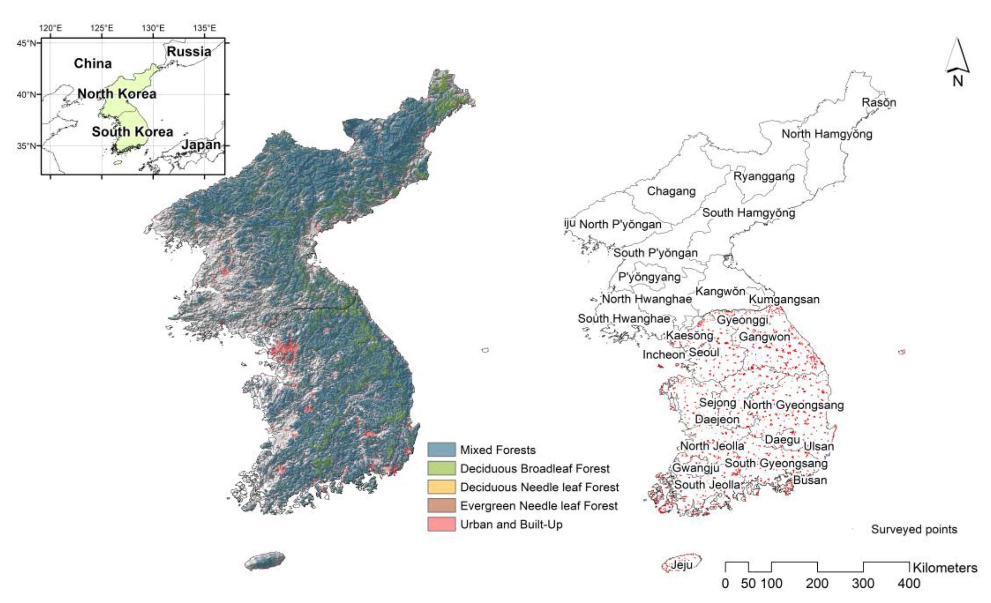
2.3. MODIS Products: NDVI and LAI (as Input Variables)

Remote sensing data efficiently record reflected energy over extended and inaccessible areas using sensors on aircraft or spacecraft, while also providing information on the spatial variability of reflectance periodically. Over the past decade, users have had opportunities to access data acquired from a variety of Earth-observing sensors. The Moderate Resolution Imaging Spectroradiometer (MODIS) is one of the most widely used remote sensing instruments aboard the Terra and Aqua satellites (https://modis.gsfc.nasa.gov/ (accessed on 24 June 2021)). With a 2330 km swath, MODIS can observe the Earth’s surface every 1 to 2 days, using an enhanced spectral resolution sensor in 36 spectral bands. Along with low-level MODIS products, diverse higher-level products for land, atmosphere, cryosphere, and ocean color applications have been distributed to the science and applications community [55]. Two MODIS sensors have sun-synchronous, near-polar circular orbits and observe the same regions 3 hours apart (Terra and Aqua are timed to cross the equator at 10:30 (from north to south) and 13:30 (from south to north), respectively).
Productivity measures calculated from remote sensing technology may be highly correlated to species richness [25]. Remote sensing indices provide a quantitative proxy of environmental phenomena as an alternative to in-situ measurements. Indices such as NDVI and leaf area index (LAI) that emphasize spectrally unique characteristics of the targets of interest have been developed for application of remote sensing data to vegetation dynamics. We used NDVI and LAI products, which may have high correlations with species richness [56], among the various regularly produced MODIS land products quantifying vegetation richness. NDVI quantifies vegetation by utilizing the spectral characteristics of green vegetation, which strongly reflects in the near-infrared range but absorbs in the red or blue wavelength region, and the value always falls between −1 and 1 (note: a negative NDVI indicates dead plants or inorganic objects, while a positive value indicates live plants, with those close to 1 being healthier) [57]. The NDVI is retrieved from daily atmosphere-corrected bidirectional surface reflectance using a specific compositing method to remove low quality data, and is widely used in all ecosystems and climates, and in natural resource management studies [58]. Leaf area index, which is defined as the one-sided green leaf area per unit ground area, is an important structural property of vegetation and characterizes plant canopies, representing foliage vigor [59]. While NDVI can be formulated by a simple difference/sum ratio, LAI is measured by a direct and destructive method, which is time-consuming [60]. LAI is mainly derived from a look-up-table that exploits the spectral information of the MODIS red and near-infrared surface reflectance, and a 3D radiative transfer equation [61].
In this study, we used the 16-day composite NDVI product (MOD13A1 and MYD13A1) at a resolution of 15 arcseconds and a combined 8-day composite LAI product (MCD15A2) at 15 arcseconds. However, since the MCD15A2 data contain many missing values because of high cloud cover, and to match the temporal resolution of the NDVI product, we converted them to 16-day composite images. To be consistent with the species richness results in South Korea, these NDVI and LAI data were then resampled at a spatial resolution of 30 arcseconds. The data were downloaded from the Land Processes Distributed Active Archive Center (LP DAAC; https://lpdaac.usgs.gov/ (accessed on 24 June 2021)) and processed using the MODIS Reprojection Tool to convert the map projection and to create mosaic images. To cover the entire Korean Peninsula, 3 images (h27v04, h27v05, and h28v05 of MODIS’s Sinusoidal Tile Grid) were composited.

2.4. Deep Learning-Based Species Richness Model

An artificial neural network mimics the learning process of the human brain and then is expanded to deep learning using deeper network architecture [26]. From an applied perspective, DL networks are able to automatically learn arbitrary complex mappings from inputs to outputs, and they offer promise for problems with complex nonlinear and multivariate regression.
Among the various types of DL architectures, multilayer perceptron (MLP) is the most practical and typical type of feedforward neural network and is effective for solving regression problems [62]. However, MLP is now deemed insufficient for modern advanced computer vision tasks. As an alternative, there is increased interest in convolutional neural networks (CNNs), which are more effective at analyzing image data [63], since they use spatial information and sparsely (partially) connected layers instead of MLP’s fully connected layers. Although we used co-registered MODIS-derived NDVI and LAI images collected in 2009 as inputs, there were many missing values at different pixel locations and times due to high cloud cover. In CNN architecture, these missing values could hinder both model training and proper inference. Therefore, in consideration of our data characteristics and the objectives of this study, pixel-wise MLP was used to estimate species richness. Multilayer perception comprises more than one perceptron, which consists of an input layer to receive the signal, an output layer that makes a decision, and one in between those two, and is capable of learning any continuous mapping function from the hierarchical or multilayered structure of the networks. Figure 3 illustrates the network architecture of MLP used in this study.
The input variables are the compiled MODIS-derived NDVI and LAI time-series ( x = [ x N D V I 1 ,   x N D V I 2 , ,   x N D V I i ,   x L A I 1 ,   x L A I 2 , ,   x L A I i ,   i = 23 ] )   collected in 2009, the middle year of the period when the species surveys were conducted, and which may have a high correlation with species richness. The output layer (y) is a value of species richness derived from S-SDMs. At each pixel location where no missing values existed, we obtained approximately 500,000 samples of x and y in South Korea for model training and testing. TensorFlow (https://tensorflow.org (accessed on 24 June 2021)), which is an end-to-end open source platform for DL, was used to develop our species richness estimation model.
In developing DL models, there are several hyperparameters that need to be tuned prior to training the model, but there are common sets of rules or heuristics governing parameter tuning. After iterative grid search parameter tuning, using a small subset of our data, 5 hidden layers ( H j , j = 1 ,   2 ,   , 5 ) were used, and the number of neurons (n) in each hidden layer was 64, 128, 256, 128, and 64, respectively. The hidden layers were stacked one by one to transfer the input signals to the deeper layer, which could extract hidden and unknown features related to species richness. We chose the RMSprop stochastic descent optimizer with the default parameters [64], and a rectified linear unit (ReLU) as a nonlinear activation function because of its promising performance in the literature [65]. Dropout layers with a rate of 0.2 were added to each hidden layer to prevent model overfitting [66]. The L1 loss function, also known as the least absolute error, was used because it is not sensitive to outliers and is intuitive. The detailed MLP model structure is described in Figure 3a.
To develop a geographically more robust estimation model due to the lack of survey data in North Korea, stacked species richness training data for South Korea were divided into quadrants (NE, NW, SE, and SW). For each quadrant of South Korea, we developed 4 MLPs using 3 subsets as the training set and the other set as the testing set. For example, as illustrated in Figure 3b, MLP 1 used the NW, SW, and SE datasets as the training sets and the SW dataset as the testing set. In MLP 2, the NE, SW, and SE datasets were used to train and the NW dataset was used to test. A randomly selected 20% of the training samples were used as validation data to determine the models’ performance and to minimize overfitting for unseen data. Therefore, we obtained 4 potential plant species richness models according to the geographical quadrants of South Korea. To evaluate the statistical model performance, estimations from the test set of each MLP model were combined, indicating that the combined statistical accuracies were calculated from the unseen data. For the final inference of the potential plant species richness of the entire Korean Peninsula at a resolution of 15 arcseconds, the resolution of the input NDVI and LAI products, and the results from all MLP branches were ensembled.
The training process was performed for a number of iterations in which all the training data were exposed to the network until the loss function reached its minimum value. The model score reached its maximum after approximately 5000 iterations with a NVIDIA Titan X GPU (3584 CUDA cores). The number of trainable parameters was 85,569 and the computational run-time was approximately 4 h with a training batch size of 1024.
Deep learning approaches have shown promising results in many scientific applications [67,68] but do not always guarantee better outcomes [69,70]. Therefore, we compared the performance of the proposed DL model with a RF regression model as a baseline, since RF showed reasonable results and is popular in various machine learning applications [71]. To determine the best values of the hyperparameters (number of trees, maximum tree depths, and the maximum number of features) in the RF model, a grid search was used.
Due to the unique characteristics of neural networks, which solve problems by exploiting the hidden relationships inherent in multiple input variables, it was difficult to physically quantify the importance of the input variables. As an alternative, we performed a statistical feature importance test (SFIT) to explain which feature had the greatest significance in the species richness retrievals and to determine the optimized features in an operational retrieval system. For the SFIT, a single feature was randomly shuffled, while all the other features were kept constant. We iterated this process by changing the test variable. The feature importance shows the extent to which the model performance decreased with random shuffling. In this study, we used the root mean square error (RMSE) as the performance metric.

2.5. Independent Validation of Species Richness

Finally, we evaluated our two model results, S-SDMs and DL species richness, by comparing the species richness obtained from independent tree plot datasets from the Korea Forest Service [72]. We calculated species richness using grids with a 10 km resolution after sensitivity analysis at different resolutions. We then calculated the overall correlation and local correlations between the species richness from the independent datasets and the results from the S-SDMs and DL species richness model. For direct comparisons, the model results were resampled at 10 km by pooling a median value of the corresponding pixels within a 10 km grid and comparing them with the results using the independent datasets. To calculate the local correlations, we defined a 3 × 3 square focal area (30 km × 30 km) for each grid, using a moving window to define the spatial ranges for correlations.

3. Results

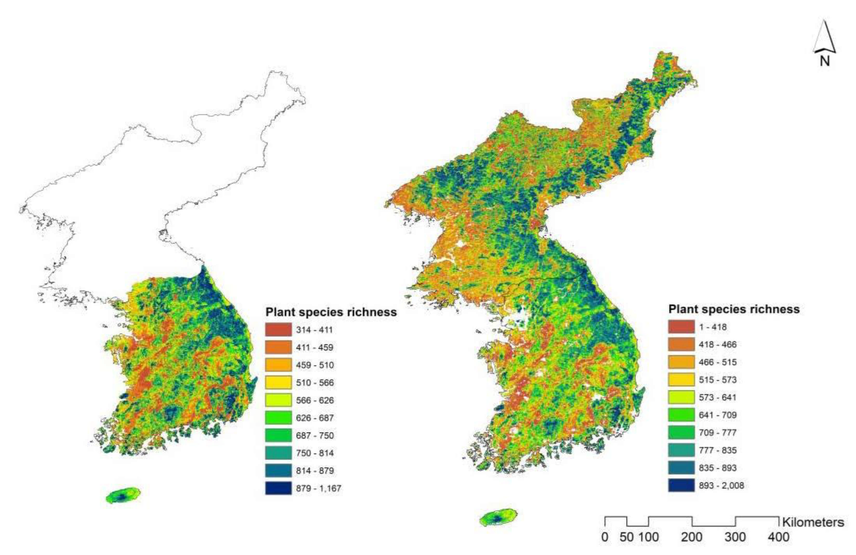
3.1. Species Richness Estimation from S-SDMs

The mean AUC and mean Boyce index of 1574 plant species were 0.77 (±0.11 SD) and 0.73 (±0.18 SD), respectively (Table S1, see Supplementary Materials). When we stacked the probability-based SDM results of 1574 species, the 30-arcsecond cell with the highest potential number of species richness had 1167 species. This was in the middle of Jeju Island, the largest island located in southernmost South Korea (Figure 4). S-SDMs predicted the highest species richness to be in the northeastern part of South Korea (Gangwon Province) and Jeju Island, and the results correspond with previous literature and other studies [33,73].

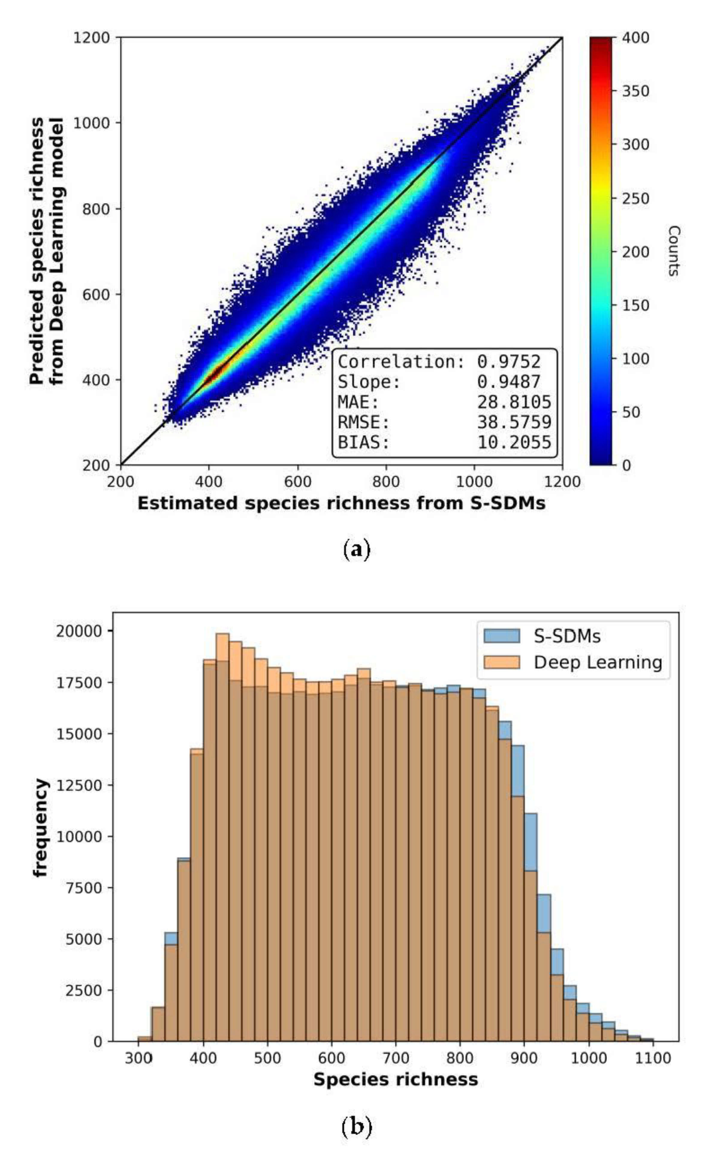
3.2. Deep Learning-Based Species Richness Estimation Model Using Remote Sensing Data

Table 1 summarizes the mean absolute error (MAE), RMSE, bias (also known as the mean error), and the Pearson’s correlation coefficient of RF and the proposed DL models. The p-values of all models from a two-sided Student’s t-test were <0.05, which means that there was a statistically significant difference between the S-SDMs-derived and RF/DL model-derived species richness at a confidence level of 95%. As shown in Table 1, all of error metrics of the proposed DL model outperformed those of the RF model. Although the RF model was computationally more efficient than the DL (approximately 1 min on a CPU (Intel E5-2699, 2.2 GHz, 22 cores) versus approximately 4 h on a GPU (NVIDIA Titan X, 3584 CUDA cores)), the error of the proposed DL model was about half that of the RF model (MAE: 28.8105 versus 61.1028; RMSE: 38.5759 versus 78.9512).
A combined scatterplot of plant species richness from the S-SDMs (PSRS-SDMs; x-axis) and DL models (PSRDL; y-axis) for the test sets, with the number of pixels denoted by the color density, shows that most data points were located around the one-to-one line (Figure 5a; black solid line), although some pixels were underestimated or overestimated. Overall, our model yielded an RMSE of 38.58 and a MAE of 28.81, with a near unity slope (0.95) in the linear regression model. The bias (mean difference between PSRS-SDMs and PSRDL) was calculated as 10.21, indicating that the proposed model slightly underestimated the potential plant species richness compared with the reference S-SDMs species richness, but the differences were small and may be handled by adjusting the slope and offset parameters in post-processing if necessary. A remarkable Pearson’s correlation coefficient (0.98) was achieved.
A histogram (Figure 5b) of PSRS-SDMs and PSRDL, with a 20 PSR bin width, shows a relative weakness in estimating PSR values between 400–600 and PSRs larger than 850. The Kullback–Leibler divergence (DKL) is often used to observe the statistical similarity of the two distributions. Although DKL is not a distance metric, it is close to zero if two distributions are similar. In this histogram, the DKL was 0.0043, indicating that the two distributions are nearly the same.
We applied the proposed model to a time-series of MODIS NDVI and LAI images acquired at a 15-arcsecond resolution to estimate plant species richness for both North and South Korea (Figure 4, right), whereas Figure 4 (left) is the reference S-SDM results for South Korea at a resolution of 30 arcseconds. For South Korea, the DL-predicted richness maps exhibited high agreement with the reference S-SDM results, which is similar to the statistical comparisons in Figure 5. There are some missing values in the predicted map (Figure 4, right), but these are mostly areas of large cities or missing values in the input NDVI or LAI images due to clouds. Based on quantitative and qualitative analysis of the S-SDMs results in South Korea, the MODIS LAI and NDVI time-series data were successfully integrated into the proposed DL model to estimate species richness. The distribution of species richness values near the border between North and South Korea showed continuous values. Forested areas in the eastern part of the Korean Peninsula showed high species richness, while low concentrations were in urban areas in the west (Figure 1). Cold highland areas in the north also showed relatively low richness values.

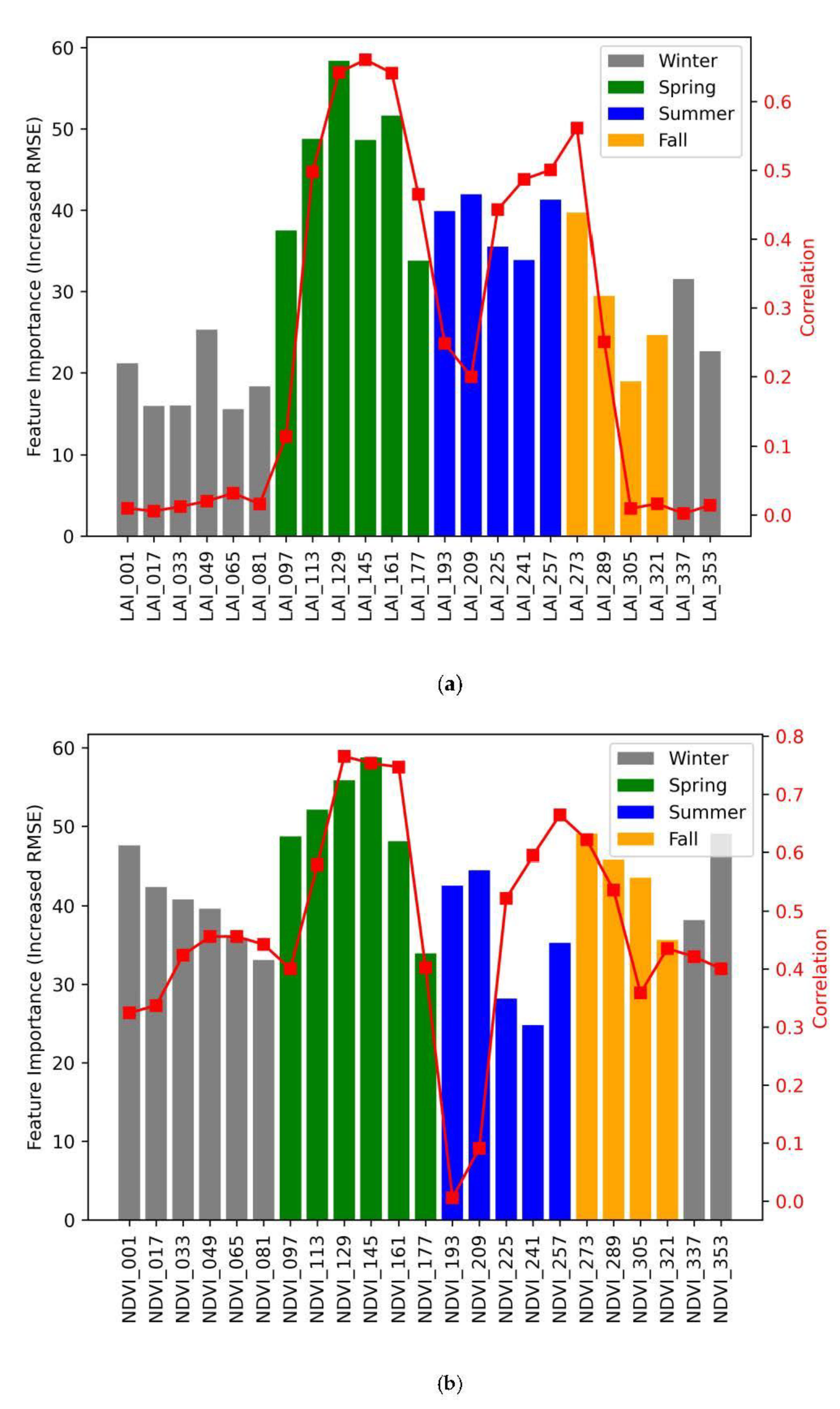
3.3. Statistical Feature Importance

Figure 6 shows the increased RMSE values obtained by the SFITs of the input features, which were calculated after 10 replications of the tests, with the Pearson’s correlation coefficients of each feature (red lines). A more important feature has a higher increased RMSE value. Table 2 summarizes the average feature importance according to the feature sources and seasons, with the correlation coefficients. We divided the input features according to the seasonal characteristics of the Korean Peninsula. Overall, NDVI-related features were generally more important than LAI features (32.64 versus 42.32). The features in the growing season (i.e., spring) exhibited greater feature importance than those of the other seasons in both the LAI and NDVI feature groups. Highly correlated features generally had higher statistical feature importance values, but were not proportional to each other.

3.4. Independent Validation of Species Richness

Species richness at a 10-km resolution using the independent South Korea datasets was high in the middle of Jeju Island, in southern mountainous areas, and in the northeastern part of South Korea (Figure 7). This is similar to the species richness results from the two species richness models (Figure 8). The overall Pearson’s correlation between the two species richness values was 0.49 for the species richness from S-SDMs and 0.47 from the DL model. From the local correlation map, we identified that positive correlations appeared in almost all regions (Figure 8). We found that the negative correlations along coastal and boundary lines, especially with the DL model results, mostly had to do with missing values from the input MODIS images.

4. Discussion

Biodiversity data are lacking in many parts of the world [24,25]. In order to overcome this limitation, deep learning, which is one of the techniques of machine learning, was applied to multitemporal satellite remote sensing data that are globally available. By DL combining the modeled richness estimations and remote sensing data, we increased the resolution of potential plant species richness maps for the Korean Peninsula to 15 arcseconds, including the large unreported area of North Korea, and maintained statistical accuracy. Since species richness represents a basic indicator for effective conservation and restoration, our results can provide resource managers and planners with maps that show areas in need of active conservation or restoration, even in regions that have not been sufficiently investigated. Threats to biodiversity are global problems [74], but the spatial gaps in scientific information make actions less reliable, because of socioeconomic status, history, culture, geography, and scientific interests [14]. Our novel data fusion approach shows potential for overcoming these data limitations.

4.1. Deep Learning-Based Species Richness Estimation

Based on our results in Table 1, the proposed DL-based model exhibited a better estimation capacity for plant species richness from remote sensing time-series data than the widely used RF model. Pau et al. [75] identified that there was no direct relationship between NDVI and species richness using the mean NDVI values of a 10-year period. However, it is worth noting that the DL model successfully captured the inherent relationships between 46 remote sensing-based input features and the species richness from the S-SDMs. An ensemble of spatially validated models using quarterly geographic datasets confirmed that the DL model was spatially robust, at least within South Korea. In light of the size and ecosystems of the Korean Peninsula and the spatial robustness of the proposed model, it could be used to estimate the spatial patterns of plant species richness in North Korea, as shown in visual inspections of Figure 4 (right).
Plant species richness may be related to a variety of factors, including temperature, light and water availability, and environmental heterogeneity [76]. We found that the average feature importance of LAI and NDVI in spring were the two most important feature groups, marking the onset of vegetation growth, while the fall months, when deciduous plants start dropping their leaves, were the most insignificant months for LAI (Table 2). However, NDVI features in the fall and winter months were more critical than the fall and winter LAI features. The high coverage of evergreen forests in the Korean Peninsula (approximately 30%) may explain the relatively high feature importance of fall and winter NDVI [77].
The relationship between LAI and NDVI is not clear. As seen in Figure 6, LAI or NDVI, at a specific time, particularly DOY 129–161, had relatively high agreement with the species richness values. However, exploiting a single LAI or NDVI feature was limited in terms of correctly retrieving the species richness values. Highly correlated features did not always guarantee high feature importance. For example, LAI337, NDVI193, and NDVI209 had very low correlation coefficients (less than 0.1), but they were statistically important in the DL model. NDVI features from DOY 225–257 were highly ranked features in the single feature correlation tests, but their feature importance was ranked at the bottom of the graph. Thus, it is difficult to say that there is a linear relationship between species richness and the correlation coefficient of a single feature. However, incorporating multiple features into the state-of-the-art DL framework proposed in this study could define the inherent relationships between species richness and remote sensing time-series data, and then estimate species richness with the accuracy level of the S-SDMs model. It seems that 46 features may be redundant, but the lack of negative feature importance in Figure 6 indicates that each feature plays a specific role in improving the species richness model in hidden networks.
Although previous studies investigated biodiversity using high-resolution airborne/spaceborne LiDAR and multispectral/hyperspectral data for local areas [29,30,31,78,79], data acquisition is challenging. Our proposed model used easy-to-access MODIS imagery to develop a species richness estimation model over extended and inaccessible regions by combining surveyed data, and further improved the spatial resolution of the species richness map.

4.2. Limitations and Recommendations

We validated our S-SDM- and DL-based species richness models using independent tree plot data. Although the independent data we used were only for trees, we found a moderate positive correlation between these species richness measures. As it can be seen in Figure 7, the area that has not been surveyed in the tree plot data is widely displayed, using smaller grids than 10 km produces many empty areas, and using larger grids generalized the richness pattern excessively [80]. There are widespread areas that have not been surveyed and it is difficult to evaluate the species richness of a large area depending only on surveys. In addition, in the local correlation map (Figure 8), most of the areas with negative correlations appear around coastal or administrative boundaries. This might be due to the differences in the resolution and the calculation methods of the two species richness sets. Therefore, it is necessary to use appropriate remote sensing data as inputs to the richness model to compensate for data scarcity according to the estimation’s purpose. Moreover, we may be able to further validate the S-SDM- and DL-based plant richness models in different ways. For example, area-specific plant surveys, targeted systematic surveys such as the forest tree survey used here, and herbarium or global species presence records such as GBIF and iNaturalist could be used to compare the S-SDM and DL models’ predictions at certain spots, either for subsets of the entire plant species richness (e.g., trees) or for the presence of individual species. While, in this study, we compared the overall pattern of species richness from each model and data source, it would also be possible to use a point-based or small area-based approach to assess the overall accuracy of our modeled approaches.
We were able to obtain a very detailed level of species richness, but it was greatly affected by the resolution of the remote sensing data we used. Although MODIS may be the best sensor for mapping at a global scale, it is not appropriate for observing local areas due to the low spatial resolution. Especially, NDVI shows higher correlation with species richness than LAI. NDVI can be readily derived from most remote sensing sensors, including sensors with better resolution but a narrower swath such as Landsat, WorldView, and KOMPSAT (Korean Multi-Purpose Satellite). Although the revisit cycle of high-resolution data is less frequent than MODIS, it may be possible to develop high-resolution species richness for local areas by optimizing our proposed model and the results of the feature importance test.
Regarding the DL framework, our proposed models were based on the most typical type of neural network, using pixel-wise inputs due to the characteristics of the data used in this study. As mentioned in Section 2.4, general image-based CNN architectures may not be appropriate for our data; applying one-dimensional CNN [81,82] or recurrent neural networks [83] in the temporal domain, or graph convolutional networks for handling graph structures between samples [84] should be interesting topics, as these are more advanced approaches. Additionally, super-resolution using a generative adversarial network [85] would further improve the spatial resolution of species richness map.
In addition, we quantitatively tested the proposed model using quarterly datasets acquired in 2009. Thus, we could not test the temporal robustness of the model using data from other years. One of the advantages of remote sensing data is it allows continuous data acquisition over extended areas. If we investigate and test multiple-year data, the proposed model can be further extended to an operational system to estimate and monitor plant species richness periodically. The GEO BON (the Group on Earth Observations Biodiversity Observation Network) consortium has developed the Local Biodiversity Intactness Index by combining the annual PREDICTS global biodiversity survey database and 1 km land-use maps [86]. Our study was able to provide more detailed information using a similar approach to GEO BON, and periodical application of our study is expected in terms of practicality. Moreover, our approach overcomes the limitations of SDMs’ environmental space, which can be explained only by the environmental variables used, by combining these with proxy values representing site degradation. Since many sites are not in pristine condition, especially in some parts of North Korea, developing a modification factor associated with site conditions could produce additional insights.

5. Conclusions

Species richness information provides basic clues for effective conservation and restoration, but many areas lack sufficient data for its estimation. We combined machine learning techniques in ecology and computer science to analyze remote sensing big data and estimate species richness across data-limited and inaccessible areas. Our DL-based model exhibited better estimation capacity for plant species richness than the widely used RF model. Overall, we found that NDVI related features in growing season are generally more important than LAI features for estimating plant species richness. Our methods are readily applicable to other regions, but the results may depend on the structure of the remote sensing data used. Thus, future studies using high-resolution remote sensing time-series data could provide more detailed information for effective conservation and restoration planning.

Supplementary Materials

The following are available online at https://www.mdpi.com/article/10.3390/rs13132490/s1. Table S1: Evaluation of the species distribution models using AUC and the Boyce index for 1574 plant species.

Author Contributions

Conceptualization, H.C. and J.C.; methodology, H.C., J.C., and J.H.T.; software, H.C. and J.C.; validation, H.C. and J.C.; resources, H.C. and J.C.; writing—original draft preparation, H.C. and J.C.; writing—review and editing, H.C., J.C., and J.H.T.; visualization, H.C. and J.C.; project administration, H.C.; funding acquisition, H.C. All authors have read and agreed to the published version of the manuscript.

Funding

This work was supported by the National Research Foundation of Korea (NRF) grant funded by the Korean government (MSIT) (No. 2019R1G1A1005770 and No. 2021R1A4A1025553) and by the Korea Polar Research Institute grant (No. PE21420). The APC was funded by Seoul National University.

Acknowledgments

The authors thank Chin-Sung Chang for comments on the manuscript and thank the three anonymous referees for constructive comments on the initial manuscript.

Conflicts of Interest

The authors declare no conflict of interest. The funders had no role in the design of the study; in the collection, analyses, or interpretation of data; in the writing of the manuscript; or in the decision to publish the results.

References

  1. Gotelli, N.J.; Colwell, R.K. Quantifying biodiversity: Procedures and pitfalls in the measurement and comparison of species richness. Ecol. Lett. 2001, 4, 379–391. [Google Scholar] [CrossRef] [Green Version]
  2. Pereira, H.M.; Ferrier, S.; Walters, M.; Geller, G.N.; Jongman, R.H.G.; Scholes, R.J.; Bruford, M.W.; Brummitt, N.; Butchart, S.H.M.; Cardoso, A.C.; et al. Essential biodiversity variables. Science 2013, 339, 277–278. [Google Scholar] [CrossRef] [PubMed] [Green Version]
  3. Wich, S.A.; Koh, L.P. Conservation Drones: Mapping and Monitoring Biodiversity; Oxford University Press: Oxford, UK, 2018. [Google Scholar]
  4. La Sorte, F.A.; Aronson, M.F.; Lepczyk, C.A.; Horton, K.G. Area is the primary correlate of annual and seasonal patterns of avian species richness in urban green spaces. Landsc. Urban Plan. 2020, 203, 103892. [Google Scholar] [CrossRef]
  5. Rocchini, D.; Balkenhol, N.; Carter, G.A.; Foody, G.; Gillespie, T.W.; He, K.S.; Kark, S.; Levin, N.; Lucas, K.; Luoto, M.; et al. Remotely sensed spectral heterogeneity as a proxy of species diversity: Recent advances and open challenges. Ecol. Inform. 2010, 5, 318–329. [Google Scholar] [CrossRef]
  6. Gotelli, N.J.; Colwell, R.K. Estimating species richness. In Biological Diversity: Frontiers in Measurement and Assessment; Oxford University Press: Oxford, UK, 2011; Volume 12, pp. 39–54. [Google Scholar]
  7. Benito, B.M.; Cayuela, L.; Albuquerque, F.S. The impact of modelling choices in the predictive performance of richness maps derived from species-distribution models: Guidelines to build better diversity models. Methods Ecol. Evol. 2013, 4, 327–335. [Google Scholar] [CrossRef]
  8. Rocchini, D.; Marcantonio, M.; Ricotta, C. Measuring Rao’s Q diversity index from remote sensing: An open source solution. Ecol. Indic. 2017, 72, 234–238. [Google Scholar] [CrossRef]
  9. Scholes, R.J.; Gill, M.J.; Costello, M.J.; Sarantakos, G.; Walters, M. Working in networks to make biodiversity data more available. In The GEO Handbook on Biodiversity Observation Networks; Walters, M., Scholes, R.J., Eds.; Springer: Cham, Switzerland, 2017; pp. 1–17. [Google Scholar]
  10. Kühl, H.S.; Bowler, D.E.; Bösch, L.; Bruelheide, H.; Dauber, J.; Eichenberg, D.; Eisenhauer, N.; Fernández, N.; Guerra, C.A.; Henle, K.; et al. Effective biodiversity monitoring needs a culture of integration. One Earth 2020, 3, 462–474. [Google Scholar] [CrossRef]
  11. Guralnick, R.P.; Hill, A.W.; Lane, M. Towards a collaborative, global infrastructure for biodiversity assessment. Ecol. Lett. 2007, 10, 663–672. [Google Scholar] [CrossRef] [Green Version]
  12. Turner, W. Sensing biodiversity. Science 2014, 346, 301–302. [Google Scholar] [CrossRef]
  13. Schmeller, D.S.; Böhm, M.; Arvanitidis, C.; Barber-Meyer, S.; Brummitt, N.; Chandler, M.; Chatzinikolaou, E.; Costello, M.J.; Ding, H.; García-Moreno, J.; et al. Building capacity in biodiversity monitoring at the global scale. Biodivers. Conserv. 2017, 26, 2765–2790. [Google Scholar] [CrossRef] [Green Version]
  14. Amano, T.; Lamming, J.D.L.; Sutherland, W.J. Spatial gaps in global biodiversity information and the role of citizen science. Bioscience 2016, 66, 393–400. [Google Scholar] [CrossRef] [Green Version]
  15. Elith, J.; Leathwick, J.R. Species distribution models: Ecological explanation and prediction across space and time. Annu. Rev. Ecol. Evol. Syst. 2009, 40, 677–697. [Google Scholar] [CrossRef]
  16. Grenié, M.; Violle, C.; Munoz, F. Is prediction of species richness from stacked species distribution models biased by habitat saturation? Ecol. Ind. 2020, 111, 105970. [Google Scholar] [CrossRef]
  17. Turner, W.; Rondinini, C.; Pettorelli, N.; Mora, B.; Leidner, A.; Szantoi, Z.; Buchanan, G.; Dech, S.; Dwyer, J.; Herold, M.; et al. Free and open-access satellite data are key to biodiversity conservation. Biol. Conserv. 2015, 182, 173–176. [Google Scholar] [CrossRef] [Green Version]
  18. Madonsela, S.; Cho, M.A.; Ramoelo, A.; Mutanga, O.; Naidoo, L. Estimating tree species diversity in the savannah using NDVI and woody canopy cover. Int. J. Appl. Earth Obs. Geoinf. 2018, 66, 106–115. [Google Scholar] [CrossRef] [Green Version]
  19. Pettorelli, N.; Safi, K.; Turner, W. Satellite remote sensing, biodiversity research and conservation of the future. Philos. Trans. R. Soc. B Biol. Sci. 2014, 369, 20130190. [Google Scholar] [CrossRef]
  20. Wu, J.; Liang, S. Developing an integrated remote sensing based biodiversity index for predicting animal species richness. Remote Sens. 2018, 10, 739. [Google Scholar] [CrossRef] [Green Version]
  21. Xu, H.; Wang, Y.; Guan, H.; Shi, T.; Hu, X. Detecting ecological changes with a remote sensing based ecological index (RSEI) produced time series and change vector analysis. Remote Sens. 2019, 11, 2345. [Google Scholar] [CrossRef] [Green Version]
  22. Randin, C.F.; Ashcroft, M.B.; Bolliger, J.; Cavender-Bares, J.; Coops, N.C.; Dullinger, S.; Dirnböck, T.; Eckert, S.; Ellis, E.; Fernández, N.; et al. Monitoring biodiversity in the Anthropocene using remote sensing in species distribution models. Remote Sens. Environ. 2020, 239, 111626. [Google Scholar] [CrossRef]
  23. Hernandez-Stefanoni, J.L.; Gallardo-Cruz, J.A.; Meave, J.A.; Rocchini, D.; Bello-Pineda, J.; López-Martínez, J.O. Modeling α- and β-diversity in a tropical forest from remotely sensed and spatial data. Int. J. Appl. Earth Obs. Geoinf. 2012, 19, 359–368. [Google Scholar] [CrossRef]
  24. Zarnetske, P.L.; Read, Q.D.; Record, S.; Gaddis, K.D.; Pau, S.; Hobi, M.L.; Malone, S.L.; Costanza, J.; Dahlin, K.M.; Latimer, A.M.; et al. Towards connecting biodiversity and geodiversity across scales with satellite remote sensing. Glob. Ecol. Biogeogr. 2019, 28, 548–556. [Google Scholar] [CrossRef] [Green Version]
  25. Soto-Navarro, C.; Ravilious, C.; Arnell, A.; de Lamo, X.; Harfoot, M.; Hill, S.L.L.; Wearn, O.R.; Santoro, M.; Bouvet, A.; Mermoz, S.; et al. Mapping co-benefits for carbon storage and biodiversity to inform conservation policy and action. Philos. Trans. R Soc. B Biol. Sci. 2020, 375, 20190128. [Google Scholar] [CrossRef] [Green Version]
  26. LeCun, Y.; Bengio, Y.; Hinton, G. Deep learning. Nature 2015, 521, 436–444. [Google Scholar] [CrossRef]
  27. Zhang, L.; Zhang, L.; Du, B. Deep learning for remote sensing data: A technical tutorial on the state of the art. IEEE Geosci. Remote Sens. Mag. 2016, 4, 22–40. [Google Scholar] [CrossRef]
  28. Zhu, X.X.; Tuia, D.; Mou, L.; Xia, G.-S.; Zhang, L.; Xu, F.; Fraundorfer, F. Deep learning in remote sensing: A comprehensive review and list of resources. IEEE Geosci. Remote Sens. Mag. 2017, 5, 8–36. [Google Scholar] [CrossRef] [Green Version]
  29. Lopatin, J.; Dolos, K.; Hernández, H.; Galleguillos, M.; Fassnacht, F. Comparing generalized linear models and random forest to model vascular plant species richness using LiDAR data in a natural forest in central Chile. Remote Sens. Environ. 2016, 173, 200–210. [Google Scholar] [CrossRef]
  30. Hakkenberg, C.R.; Zhu, K.; Peet, R.K.; Song, C. Mapping multi-scale vascular plant richness in a forest landscape with inte-grated LiDAR and hyperspectral remote-sensing. Ecology 2018, 99, 474–487. [Google Scholar] [CrossRef]
  31. Sun, Y.; Huang, J.; Ao, Z.; Lao, D.; Xin, Q. Deep learning approaches for the mapping of tree species diversity in a tropical wetland using airborne LiDAR and high-spatial-resolution remote sensing images. Forests 2019, 10, 1047. [Google Scholar] [CrossRef] [Green Version]
  32. Kim, K.C. Preserving biodiversity in Korea’s demilitarized zone. Science 1997, 278, 242–243. [Google Scholar] [CrossRef]
  33. Choe, H.; Thorne, J.H.; Seo, C. Mapping national plant biodiversity patterns in South Korea with the MARS species distribution model. PLoS ONE 2016, 11, e0149511. [Google Scholar] [CrossRef]
  34. Ministry of Environment. The 3rd Master Plans for Protection of Wildlife (2016–2020); Ministry of Environment: Sejong-si, Korea, 2016. (In Korean)
  35. Dinerstein, E.; Olson, D.; Joshi, A.; Vynne, C.; Burgess, N.D.; Wikramanayake, E.; Hahn, N.; Palminteri, S.; Hedao, P.; Noss, R.; et al. An ecoregion-based approach to protecting half the terrestrial realm. Bioscience 2017, 67, 534–545. [Google Scholar] [CrossRef] [PubMed]
  36. Hernandez, P.A.; Graham, C.H.; Master, L.L.; Albert, D.L. The effect of sample size and species characteristics on performance of different species distribution modeling methods. Ecography 2006, 29, 773–785. [Google Scholar] [CrossRef]
  37. Van Proosdij, A.S.J.; Sosef, M.S.M.; Wieringa, J.J.; Raes, N. Minimum required number of specimen records to develop accurate species distribution models. Ecography 2016, 39, 542–552. [Google Scholar] [CrossRef]
  38. Hijmans, R.J.; Cameron, S.E.; Parra, J.L.; Jones, P.G.; Jarvis, A. Very high resolution interpolated climate surfaces for global land areas. Int. J. Climatol. J. R. Meteorol. Soc. 2005, 25, 1965–1978. [Google Scholar] [CrossRef]
  39. FAO; IIASA; ISRIC; ISSCAS; JRC. Harmonized World Soil Database (Version 1.2); FAO: Rome, Italy; IIASA: Laxenburg, Austria, 2012. [Google Scholar]
  40. Jarvis, A.; Reuter, H.I.; Nelson, A.; Guevara, E. Hole-Filled Seamless SRTM Data V4, International Centre for Tropical Agri-culture (CIAT). 2008. Available online: http://srtm.csi.cgiar.org (accessed on 24 June 2021).
  41. Choe, H.; Thorne, J.H.; Joo, W.; Kwon, H. The biodiversity representation assessment in South Korea’s protected area network. J. Korea Soc. Environ. Restor. Technol. 2020, 23, 77–87. [Google Scholar]
  42. Dormann, C.F.; Elith, J.; Bacher, S.; Buchmann, C.; Carl, G.; Carré, G.; Marquéz, J.R.G.; Gruber, B.; Lafourcade, B.; Leitão, P.J.; et al. Collinearity: A review of methods to deal with it and a simulation study evaluating their performance. Ecography 2013, 36, 27–46. [Google Scholar] [CrossRef]
  43. Manzoor, S.A.; Griffiths, G.; Lukac, M. Species distribution model transferability and model grain size—Finer may not always be better. Sci. Rep. 2018, 8, 7168. [Google Scholar] [CrossRef] [Green Version]
  44. Phillips, S.J.; Anderson, R.P.; Schapire, R.E. Maximum entropy modeling of species geographic distributions. Ecol. Model. 2006, 190, 231–259. [Google Scholar] [CrossRef] [Green Version]
  45. Elith, J.; Graham, C.H.; Anderson, R.P.; Dudík, M.; Ferrier, S.; Guisan, A.; Hijmans, R.J.; Huettmann, F.; Leathwick, J.R.; Lehmann, A. Novel methods improve prediction of species’ distributions from occurrence data. Ecography 2006, 29, 129–151. [Google Scholar] [CrossRef] [Green Version]
  46. Aguirre-Gutiérrez, J.; Carvalheiro, L.G.; Polce, C.; van Loon, E.E.; Raes, N.; Reemer, M.; Biesmeijer, J.C. Fit-for-purpose: Species distribution model performance depends on evaluation criteria—Dutch hoverflies as a case study. PLoS ONE 2013, 8, e63708. [Google Scholar] [CrossRef] [Green Version]
  47. Lomba, A.; Pellissier, L.; Randin, C.; Vicente, J.; Moreira, F.; Honrado, J.; Guisan, A. Overcoming the rare species modelling paradox: A novel hierarchical framework applied to an Iberian endemic plant. Biol. Conserv. 2010, 143, 2647–2657. [Google Scholar] [CrossRef]
  48. Breiner, F.T.; Guisan, A.; Bergamini, A.; Nobis, M. Overcoming limitations of modelling rare species by using ensembles of small models. Methods Ecol. Evol. 2015, 6, 1210–1218. [Google Scholar] [CrossRef]
  49. Naimi, B.; Araújo, M.B. Sdm: A reproducible and extensible R platform for species distribution modelling. Ecography 2016, 39, 368–375. [Google Scholar] [CrossRef] [Green Version]
  50. D’Amen, M.; Dubuis, A.; Fernandes, R.F.; Pottier, J.; Pellissier, L.; Guisan, A. Using species richness and functional traits predictions to constrain assemblage predictions from stacked species distribution models. J. Biogeogr. 2015, 42, 1255–1266. [Google Scholar] [CrossRef]
  51. Mateo, R.G.; Felicisimo, A.M.; Pottier, J.; Guisan, A.; Muñoz, J. Do stacked species distribution models reflect altitudinal diversity patterns? PLoS ONE 2012, 7, e32586. [Google Scholar] [CrossRef] [Green Version]
  52. Sullivan, B.L.; Wood, C.L.; Iliff, M.J.; Bonney, R.E.; Fink, D.; Kelling, S. EBird: A citizen-based bird observation network in the biological sciences. Biol. Conserv. 2009, 142, 2282–2292. [Google Scholar] [CrossRef]
  53. Scherrer, D.; Mod, H.K.; Guisan, A. How to evaluate community predictions without thresholding? Methods Ecol. Evol. 2020, 11, 51–63. [Google Scholar] [CrossRef] [Green Version]
  54. Del Toro, I.; Ribbons, R.R.; Hayward, J.; Andersen, A.N. Are stacked species distribution models accurate at predicting multiple levels of diversity along a rainfall gradient? Austral. Ecol. 2019, 44, 105–113. [Google Scholar] [CrossRef] [Green Version]
  55. Justice, C.; Townshend, J.; Vermote, E.; Masuoka, E.; Wolfe, R.; Saleous, N.; Roy, D.; Morisette, J. An overview of MODIS land data processing and product status. Remote. Sens. Environ. 2002, 83, 3–15. [Google Scholar] [CrossRef]
  56. Huete, A.R. Vegetation indices, remote sensing and forest monitoring. Geogr. Compass 2012, 6, 513–532. [Google Scholar] [CrossRef]
  57. Jensen, J.R. Remote Sensing of the Environment: An Earth Resource Perspective; Pearson Prentice Hall: Upper Saddle River, NJ, USA, 2007. [Google Scholar]
  58. Didan, K.; Munoz, A.B.; Solano, R.; Huete, A. MODIS Vegetation Index User’s Guide (MOD13 Series). Version 3.00; Vegetation Index and Phenology Lab, University of Arizona: Tucson, AZ, USA, 2015. [Google Scholar]
  59. Carlson, T.N.; Ripley, D.A. On the relation between NDVI, fractional vegetation cover, and leaf area index. Remote Sens. Environ. 1997, 62, 241–252. [Google Scholar] [CrossRef]
  60. Campillo, C.; García, M.; Daza, C.; Prieto, M. Study of a non-destructive method for estimating the leaf area index in vegetable crops using digital images. HortScience 2010, 45, 1459–1463. [Google Scholar] [CrossRef]
  61. Myneni, R.; Knyazikhin, Y.; Park, T. MCD15A2H MODIS/Terra + Aqua Leaf Area Index/FPAR 8-day L4 Global 500 m SIN Grid V006; NASA EOSDIS Land Processes DAAC: Sioux Falls, SD, USA, 2015. [CrossRef]
  62. Gardner, M.W.; Dorling, S.R. Artificial neural networks (the multilayer perceptron)—A review of applications in the at-mospheric sciences. Atmos. Environ. 1998, 32, 2627–2636. [Google Scholar] [CrossRef]
  63. Krizhevsky, A.; Sutskever, I.; Hinton, G.E. Imagenet classification with deep convolutional neural networks. Commun. ACM 2017, 60, 84–90. [Google Scholar] [CrossRef]
  64. Tieleman, T.; Hinton, G. Lecture 6.5-rmsprop: Divide the gradient by a running average of its recent magnitude. COURSERA Neural Netw. Mach. Learn. 2012, 4, 26–31. [Google Scholar]
  65. Chollet, F. Deep Learning with R; Manning Publications: Shelter Island, NY, USA, 2018. [Google Scholar]
  66. Srivastava, N.; Hinton, G.; Krizhevsky, A.; Sutskever, I.; Salakhutdinov, R. Dropout: A simple way to prevent neural networks from overfitting. J. Mach. Learn. Res. 2014, 15, 1929–1958. [Google Scholar]
  67. Bhatnagar, S.; Gill, L.; Ghosh, B. Drone image segmentation using machine and deep learning for mapping raised bog vegetation communities. Remote Sens. 2020, 12, 2602. [Google Scholar] [CrossRef]
  68. Kim, Y.J.; Kim, H.-C.; Han, D.; Lee, S.; Im, J. Prediction of monthly Arctic sea ice concentrations using satellite and reanalysis data based on convolutional neural networks. Cryosphere 2020, 14, 1083–1104. [Google Scholar] [CrossRef] [Green Version]
  69. Korotcov, A.; Tkachenko, V.; Russo, D.P.; Ekins, S. Comparison of deep learning with multiple machine learning methods and metrics using diverse drug discovery data sets. Mol. Pharm. 2017, 14, 4462–4475. [Google Scholar] [CrossRef]
  70. Joharestani, M.Z.; Cao, C.; Ni, X.; Bashir, B.; Talebiesfandarani, S. PM2.5 prediction based on random forest, XGBoost, and deep learning using multisource remote sensing data. Atmosphere 2019, 10, 373. [Google Scholar] [CrossRef] [Green Version]
  71. Fernández-Delgado, M.; Cernadas, E.; Barro, S.; Amorim, D. Do we need hundreds of classifiers to solve real world classifi-cation problems? J. Mach. Learn. Res. 2014, 15, 3133–3181. [Google Scholar]
  72. Korea Forest Service. The 6th National Forest Inventory and Monitoring; Korea Forest Service: Daejeon, Korea, 2016. [Google Scholar]
  73. Choe, H.; Thorne, J.H.; Huber, P.R.; Lee, D.; Quinn, J.F. Assessing shortfalls and complementary conservation areas for national plant biodiversity in South Korea. PLoS ONE 2018, 13, e0190754. [Google Scholar] [CrossRef]
  74. Malhi, Y.; Franklin, J.; Seddon, N.; Solan, M.; Turner, M.G.; Field, C.B.; Knowlton, N. Climate change and ecosystems: Threats, opportunities and solutions. Philos. Trans. R. Soc. B Biol. Sci. 2020, 375, 20190104. [Google Scholar] [CrossRef] [Green Version]
  75. Pau, S.; Gillespie, T.W.; Wolkovich, E.M. Dissecting NDVI-species richness relationships in Hawaiian dry forests. J. Biogeogr. 2012, 39, 1678–1686. [Google Scholar] [CrossRef]
  76. Pausas, J.G.; Austin, M.P. Patterns of plant species richness in relation to different environments: An appraisal. J. Veg. Sci. 2001, 12, 153–166. [Google Scholar] [CrossRef]
  77. Kang, J.; Suh, M.; Kwak, C. Classification of land cover over the Korean peninsula using MODIS data. Atmosphere 2009, 19, 169–182. [Google Scholar]
  78. Camathias, L.; Küchler, M.; Stofer, S.; Baltensweiler, A.; Bergamini, A. High-resolution remote sensing data improves models of species richness. Appl. Veg. Sci. 2013, 16, 539–551. [Google Scholar] [CrossRef]
  79. Cord, A.F.; Klein, D.; Gernandt, D.S.; de la Rosa, J.A.P.; Dech, S. Remote sensing data can improve predictions of species richness by stacked species distribution models: A case study for Mexican pines. J. Biogeogr. 2014, 41, 736–748. [Google Scholar] [CrossRef]
  80. Choe, H.; Thorne, J.H.; Hijmans, R.; Seo, C. Integrating the Rabinowitz rarity framework with a National Plant Inventory in South Korea. Ecol. Evol. 2019, 9, 1353–1363. [Google Scholar] [CrossRef]
  81. Ince, T.; Kiranyaz, S.; Eren, L.; Askar, M.; Gabbouj, M. Real-time motor fault detection by 1-D convolutional neural networks. IEEE Trans. Ind. Electron. 2016, 63, 7067–7075. [Google Scholar] [CrossRef]
  82. Peng, D.; Liu, Z.; Wang, H.; Qin, Y.; Jia, L. A novel deeper one-dimensional CNN with residual learning for fault diagnosis of wheelset bearings in high-speed trains. IEEE Access 2019, 7, 10278–10293. [Google Scholar] [CrossRef]
  83. Sak, H.; Senior, A.; Beaufays, F. Long short-term memory based recurrent neural network architectures for large vocabulary speech recognition. arXiv 2014, arXiv:1402.1128. [Google Scholar]
  84. Hong, D.; Gao, L.; Yao, J.; Zhang, B.; Plaza, A.; Chanussot, J. Graph convolutional networks for hyperspectral image classification. IEEE Trans. Geosci. Remote Sens. 2020, 1–13. [Google Scholar] [CrossRef]
  85. Ledig, C.; Theis, L.; Huszar, F.; Caballero, J.; Cunningham, A.; Acosta, A.; Aitken, A.; Tejani, A.; Totz, J.; Wang, Z.; et al. Photo-realistic single image super-resolution using a generative adversarial network. In Proceedings of the 2017 IEEE Conference on Computer Vision and Pattern Recognition (CVPR), Honolulu, HI, USA, 21–26 July 2017; pp. 5892–5900. [Google Scholar]
  86. GEO BON. Global Biodiversity Change Indicators. Version 1.2; Group on Earth Observations Biodiversity Observation Network Secretariat: Leipzig, Germany, 2015; 20p. [Google Scholar]
Figure 1. Topography and forest distributions on the Korean Peninsula (left), and administrative boundaries and the surveyed point locations of plants used in S-SDMs (right).
Remotesensing 13 02490 g001
Figure 2. Overview of the present study. Potential plant species richness in South Korea calculated by combining the 1574 species’ suitability estimations from species distribution models at 30-arcseconds was used as the ground truth. Multilayer perceptron (MLP) models using quarterly Moderate Resolution Imaging Spectroradiometer (MODIS)-driven Normalized Difference Vegetation Index (NDVI) and Leaf Area Index (LAI) time-series datasets in South Korea were applied to estimate the plant species richness at a 15-arcsecond resolution for the entire Korean Peninsula, including inaccessible North Korea.
Remotesensing 13 02490 g002
Figure 3. Network architecture of the species richness estimation model of the Korean Peninsula. (a) Individual network architecture of each MLP block. Here, x is the MODIS-derived NDVI and LAI time-series data at each pixel location, and y is the corresponding species richness derived from S-SDMs. (b) Overall architecture of the proposed method from quarterly geographic datasets of South Korea.
Remotesensing 13 02490 g003
Figure 4. Potential plant species richness estimated from S-SDMs in South Korea (left) and estimated by the deep learning model in the Korean Peninsula (right). Nonzero values are grouped into 10 classes in each figure; each class contains an equal number of grid cells (decile).
Remotesensing 13 02490 g004
Figure 5. Statistical accuracies of the proposed DL-based species richness model. (a) Scatterplot of S-SDMs-estimated (x-axis) and DL-estimated (y-axis) species richness values; (b) histograms of S-SDMs-estimated (blue) and DL-estimated (orange) species richness values.
Remotesensing 13 02490 g005
Figure 6. Statistical importance of input variables in feature permutation tests. (a) LAI features; (b) NDVI features. Pearson’s correlation coefficients between each feature and the species richness values are plotted as red lines. Note: the numbers in the feature names are the day of the year.
Remotesensing 13 02490 g006
Figure 7. Independent tree plot datasets (left) and species richness obtained from independent tree plot datasets (right).
Remotesensing 13 02490 g007
Figure 8. Local correlations between species richness from independent tree datasets and from S-SDMs (left) and from the deep learning model (right) in grids at a 10 km resolution.
Remotesensing 13 02490 g008
Table 1. Comparison of statistical accuracy metrics between the random forest and deep learning models.
Model TypesMAE (Mean Absolute Error)RMSE (Root Mean Square Error)BiasCorrelation
Random Forest61.102878.95120.56560.8843
Deep Learning28.810538.575910.20550.9752
Table 2. Comparison of feature importance according to the seasons (seasonal correlation coefficients from single feature tests are in parentheses).
DOY (Day of Year)LAI (Leaf Area Index)NDVI (Normalized Difference Vegetation Index)
Spring97–17746.46 (0.50)49.59 (0.61)
Summer193–25738.51 (0.38)35.06 (0.38)
Fall273–32128.19 (0.21)43.50 (0.49)
Winter1–81; 337–35320.84 (0.01)40.83 (0.41)
Average 32.64 (0.25)42.32 (0.47)
Publisher’s Note: MDPI stays neutral with regard to jurisdictional claims in published maps and institutional affiliations.

