
A Study of Two Impactful Heavy Rainfall Events in the Southern Appalachian Mountains during Early 2020, Part I; Societal Impacts, Synoptic Overview, and Historical Context

 , , and
Abstract
:1. Background
2. Methodology
2.1. Surface-Based Observations
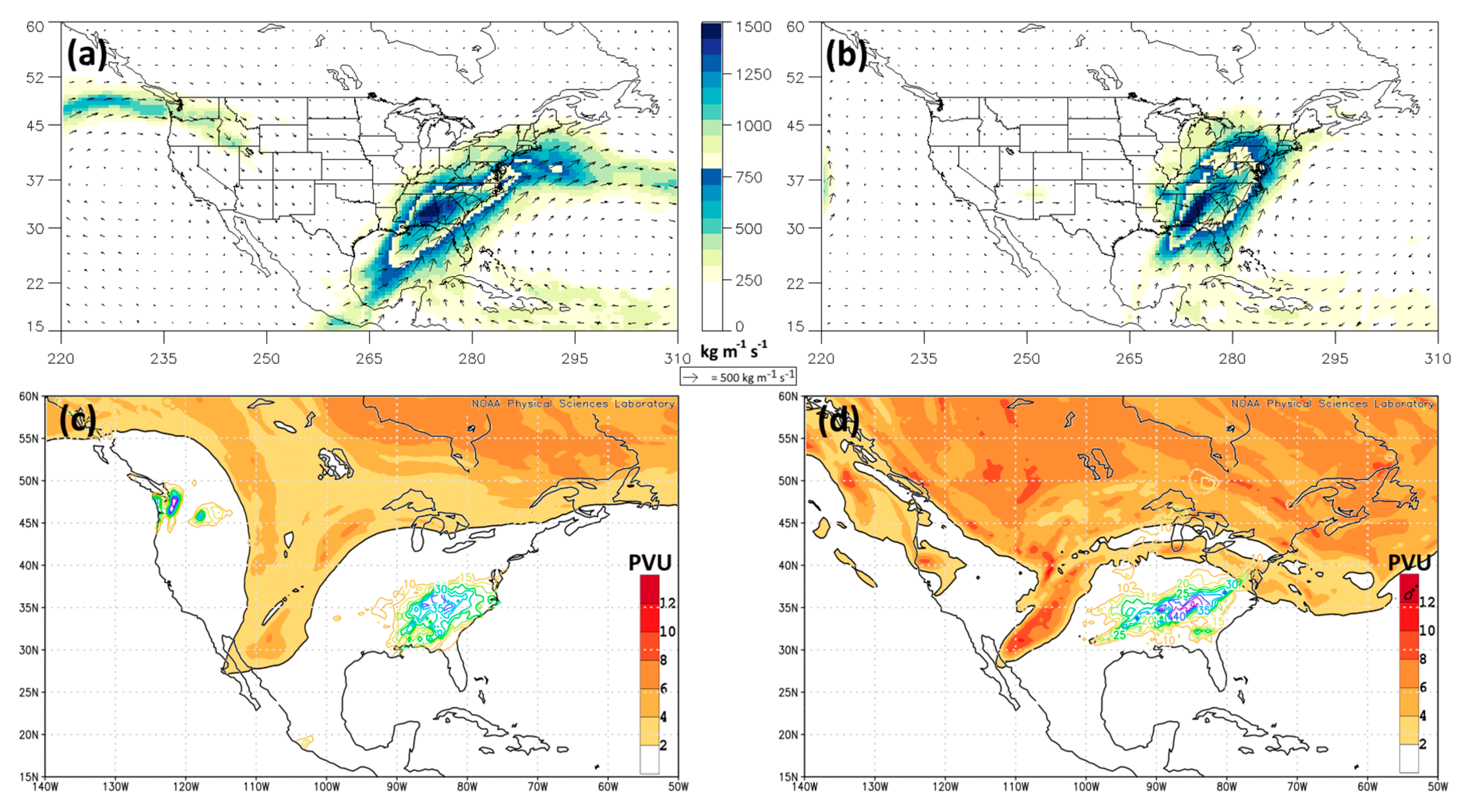
2.2. Atmospheric River Detection Algorithm
2.3. Space-Borne Observations
2.3.1. Soil Moisture
2.3.2. Precipitable Water
2.3.3. Flooding
3. Results
3.1. Societal Hazards
3.1.1. Flooding
3.1.2. Landslides
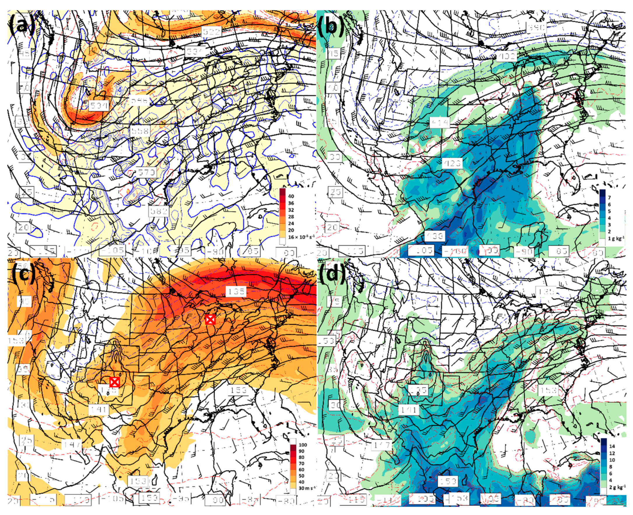
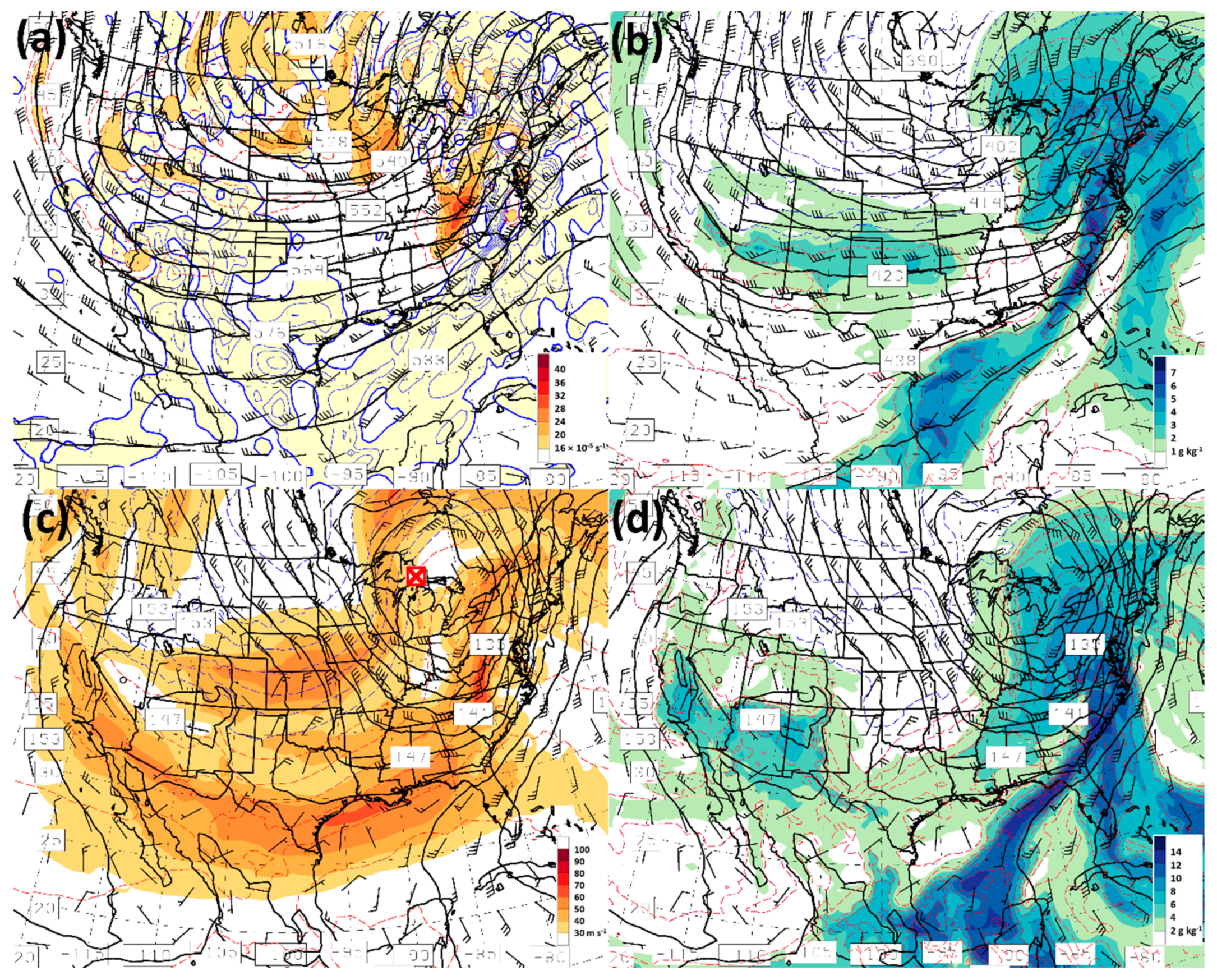
3.2. Synoptic Setting
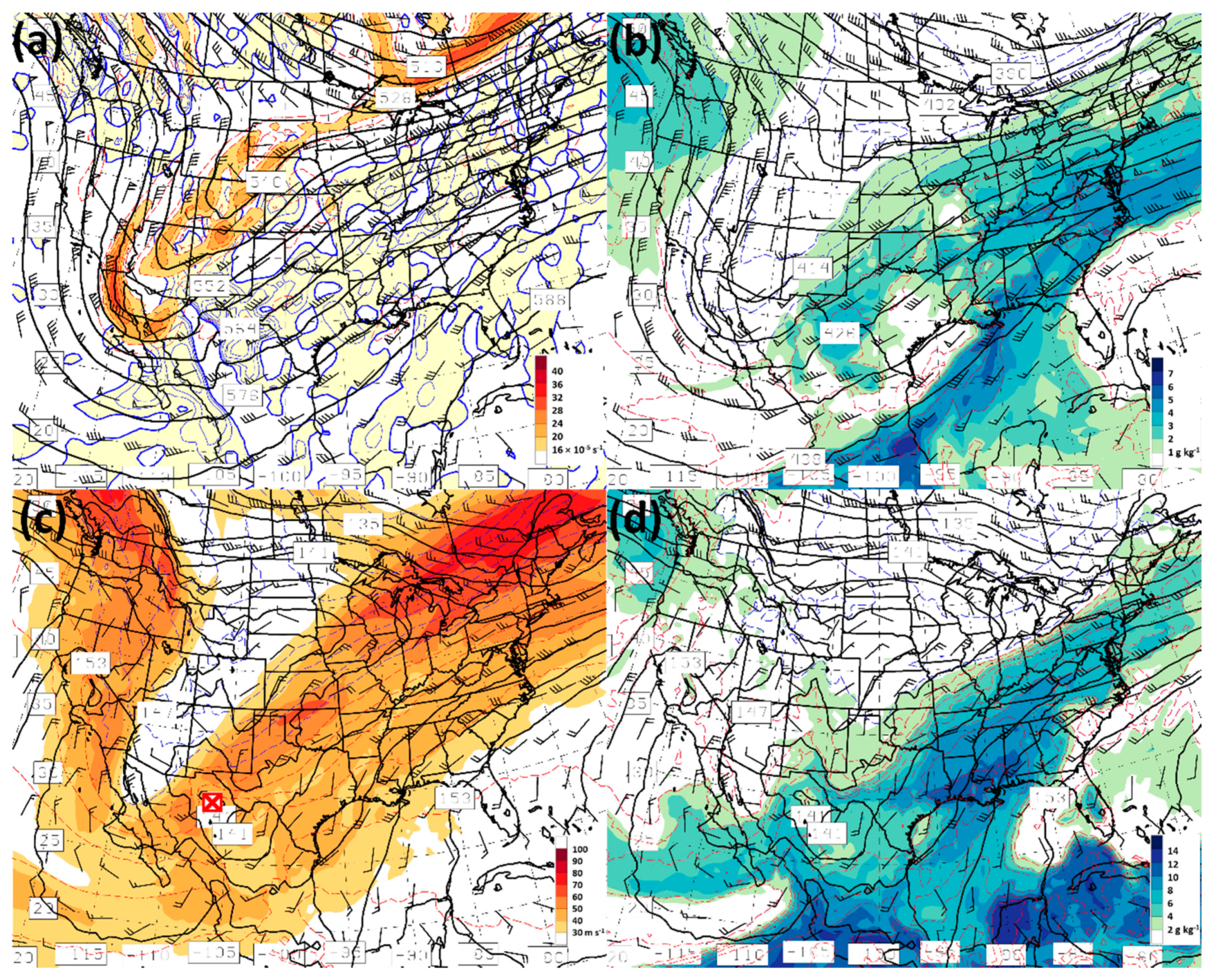
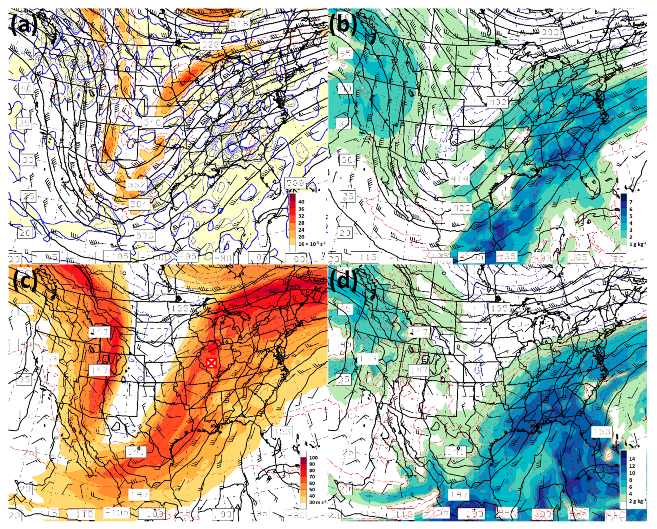
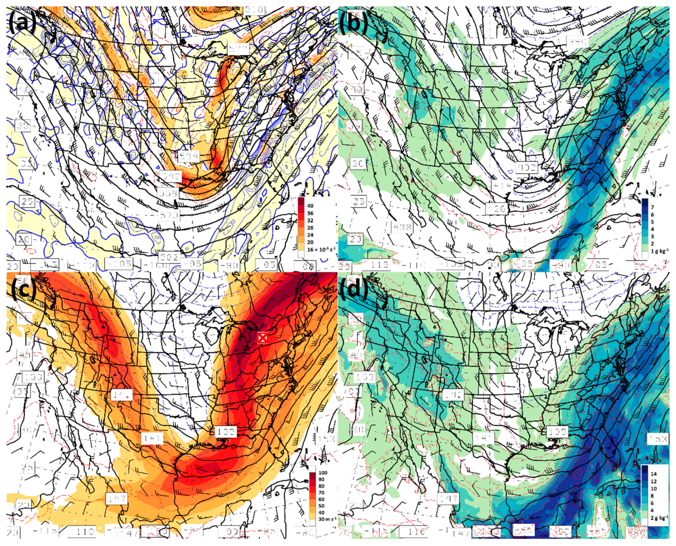
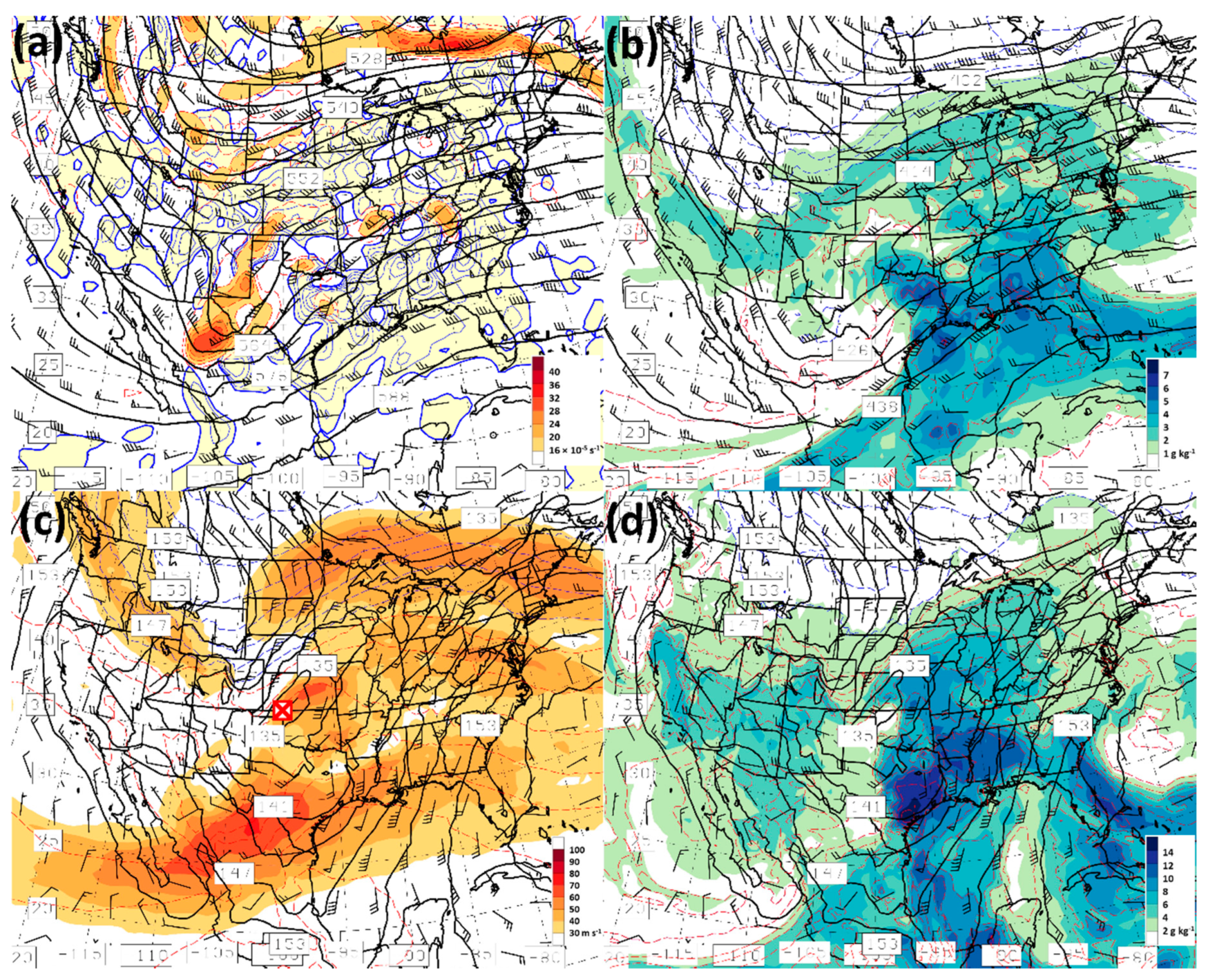
3.2.1. GFS Analyses
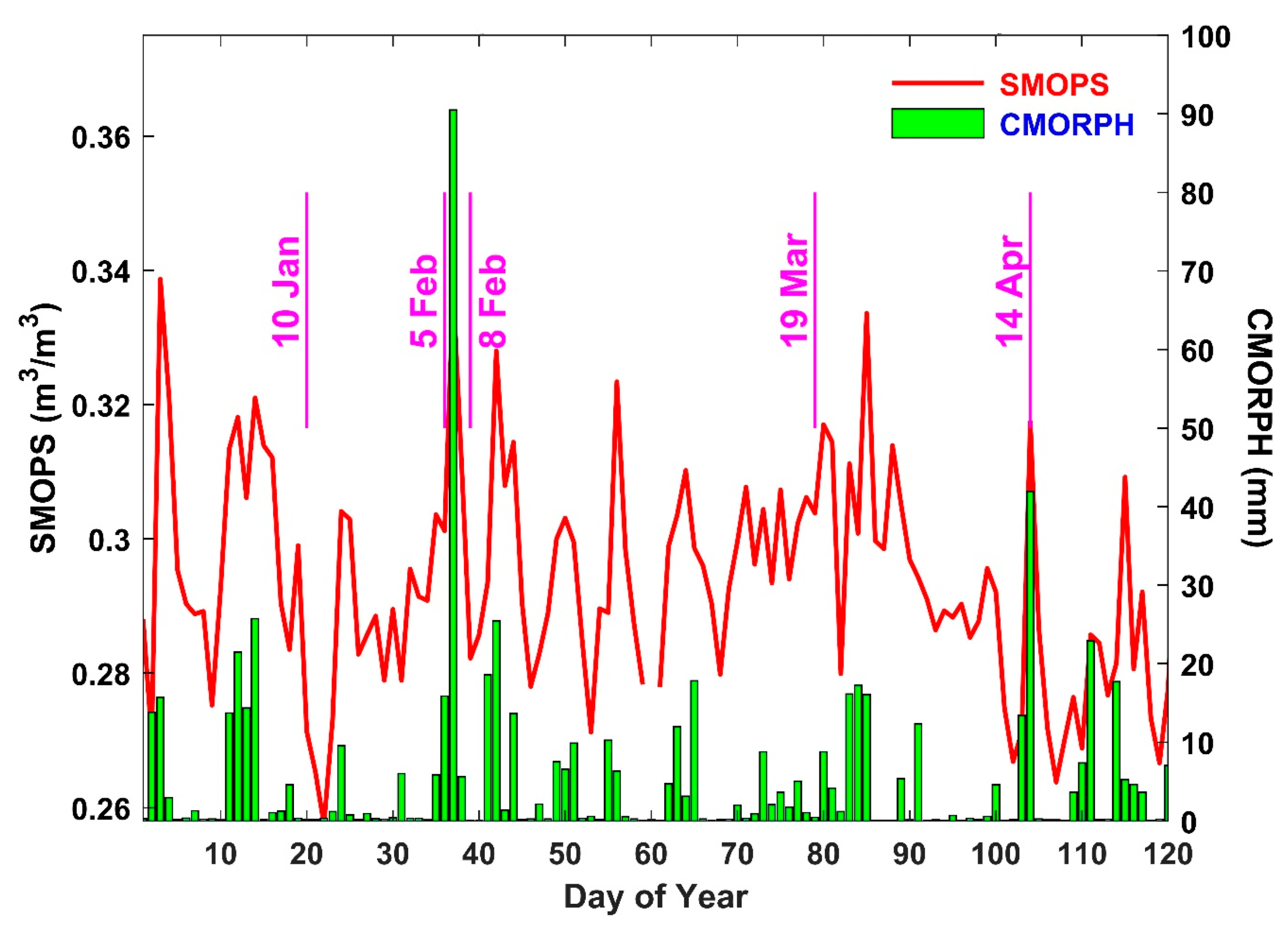
3.2.2. Soil Moisture
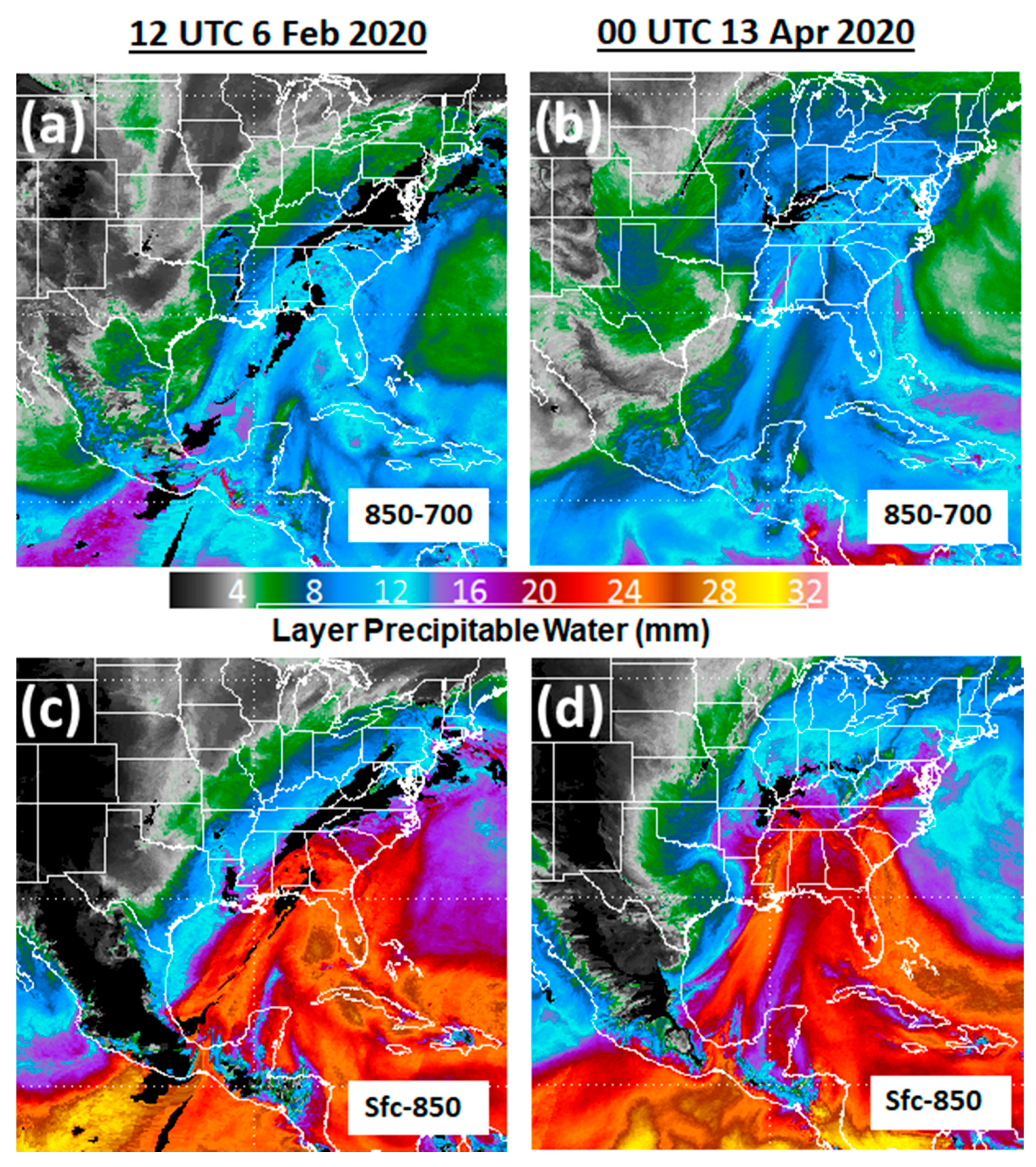
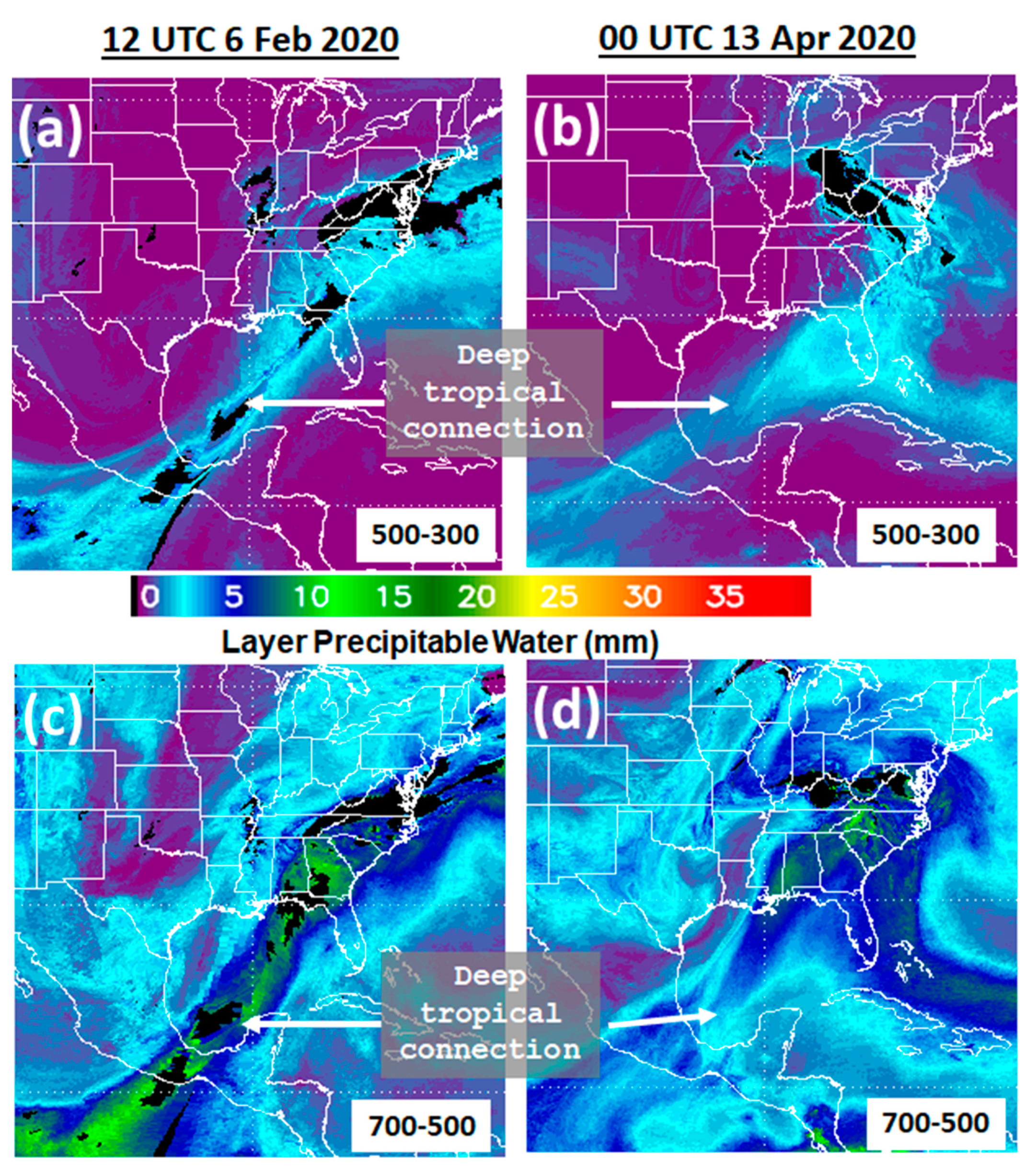
3.2.3. Blended Precipitable Water
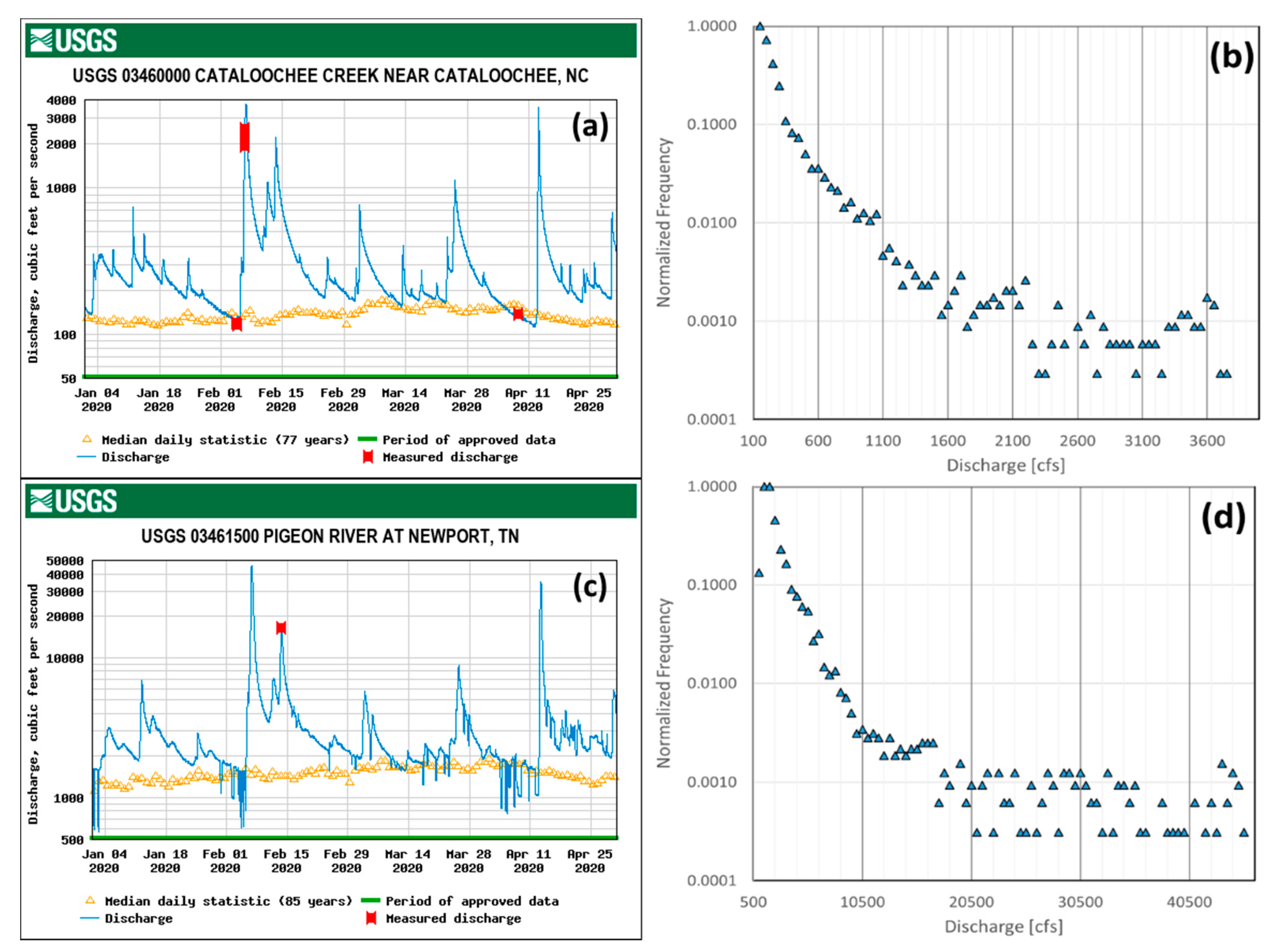
3.3. Rainfall Observations
Historical Perspective
4. Discussion
5. Conclusions
Author Contributions
Funding
Institutional Review Board Statement
Informed Consent Statement
Data Availability Statement
Acknowledgments
Conflicts of Interest
Appendix A

| Duke GSMRGN Gauge Attributes | CHLRGN Gauge Attributes | ||||||||||
|---|---|---|---|---|---|---|---|---|---|---|---|
| Gauge | Lat. | Lon. | Elev. (m) | Gauge | Lat. | Lon. | Elev. (m) | Gauge | Lat. | Lon. | Elev. (m) |
| RG002 | 35°25.5′ | 82°58.2′ | 1731 | RG109 | 35°29.7′ | 83°02.4′ | 1500 | WRG06 | 35°3.62′ | 83°25.8′ | 687 |
| RG003 | 35°23.0′ | 82°54.9′ | 1609 | RG110 | 35°32.8′ | 83°08.8′ | 1563 | WRG05 | 35°3.63′ | 83°27.9′ | 1144 |
| RG004 | 35°22.0′ | 82°59.4′ | 1922 | RG111 | 35°43.7′ | 82°56.8′ | 1394 | WRG20 | 35°3.89′ | 83°26.5′ | 740 |
| RG005 | 35°24.5′ | 82°57.8′ | 1520 | RG112 | 35°45.0′ | 82°57.8′ | 1184 | WRG31 | 35°1.96′ | 83°28.1′ | 1366 |
| RG008 | 35°22.9′ | 82°58.4′ | 1737 | RG300 | 35°43.5′ | 83°13.0′ | 1558 | WRG13 | 35°3.75′ | 83°27.4′ | 961 |
| RG010 | 35°27.3′ | 82°56.8′ | 1478 | RG301 | 35°42.3’ | 83°15.3′ | 2003 | WRG41 | 35°3.32′ | 83°25.7′ | 776 |
| RG011 | 35°23.7′ | 82°54.9′ | 1244 | RG302 | 35°43.2′ | 83°14.8′ | 1860 | WRG12 | 35°2.84′ | 83°27.5′ | 1001 |
| RG100 | 35°35.1′ | 83°04.3′ | 1495 | RG303 | 35°45.7′ | 83°09.7′ | 1490 | WRG55 | 35°2.39′ | 83°27.3′ | 1035 |
| RG101 | 35°34.5′ | 83°05.2′ | 1520 | RG304 | 35°40.2′ | 83°10.9′ | 1820 | WRG96 | 35°2.72′ | 83°26.2′ | 894 |
| RG102 | 35°33.8′ | 83°06.2′ | 1635 | RG305 | 35°41.4′ | 83°07.9′ | 1630 | ||||
| RG103 | 35°33.2′ | 83°07.0′ | 1688 | RG306 | 35°44.7′ | 83°10.2′ | 1536 | ||||
| RG104 | 35°33.2′ | 83°05.2′ | 1587 | RG307 | 35°39.0′ | 83°11.9′ | 1624 | ||||
| RG105 | 35°38.0′ | 83°02.4′ | 1345 | RG308 | 35°43.8′ | 83°10.9′ | 1471 | ||||
| RG106 | 35°25.9′ | 83°01.7′ | 1210 | RG309 | 35°40.9′ | 83°09.0′ | 1604 | ||||
| RG107 | 35°34.0′ | 82°54.4′ | 1359 | RG310 | 35°42.1′ | 83°07.3′ | 1756 | ||||
| RG108 | 35°33.2′ | 82°59.3′ | 1277 | RG311 | 35°45.9′ | 83°08.4′ | 1036 | ||||
Appendix B
| Abbreviation | Definition |
|---|---|
| AR | Atmospheric River |
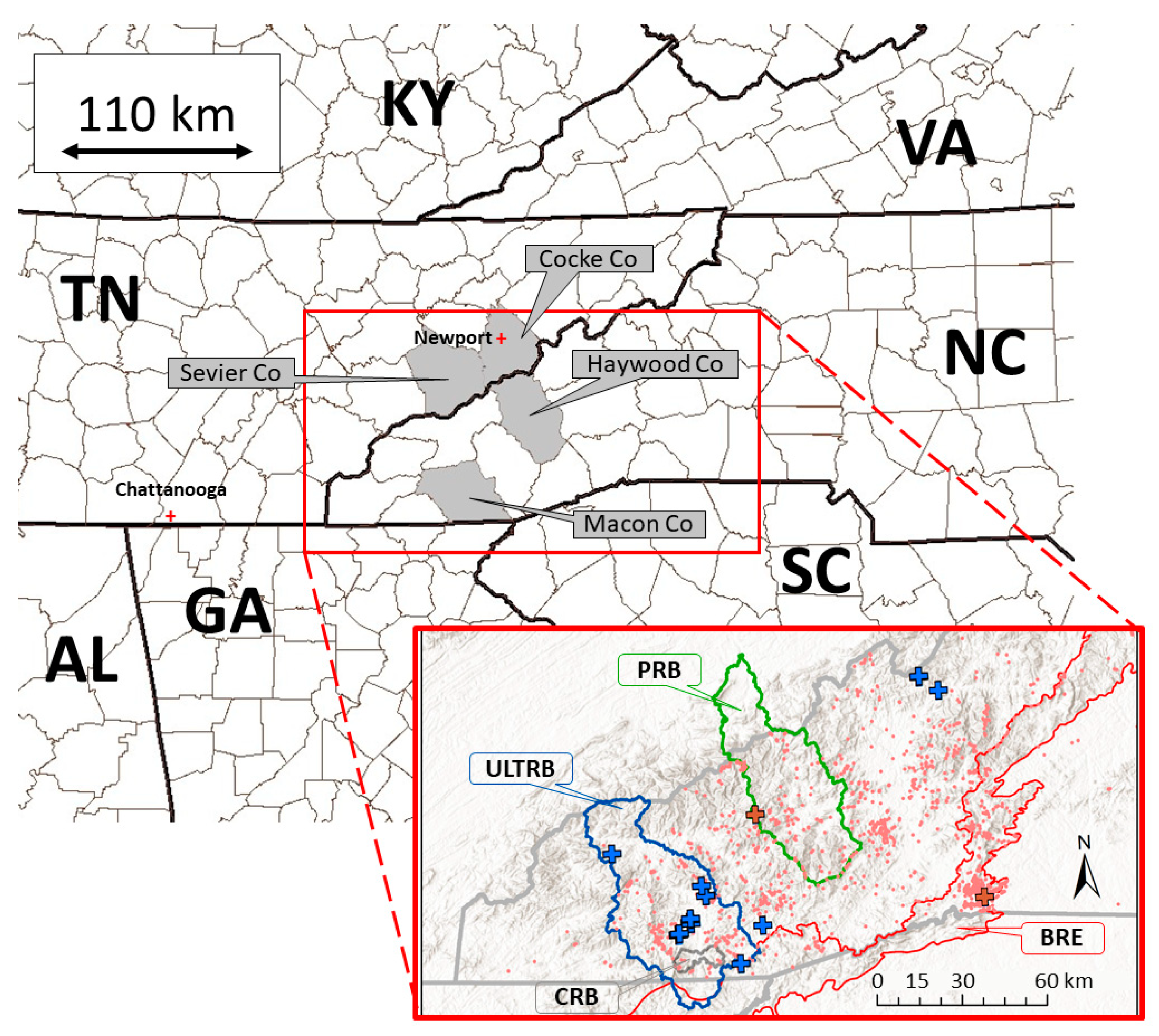
| BRE | Blue Ridge Escarpment |
| CHLRGN | Coweeta Hydrologic Laboratory Rain Gauge Network |
| CRB | Coweeta River Sub-Basin |
| Duke GSMRGN | Duke Great Smoky Mountains Rain Gauge Network |
| ERTC | Elevated Rain Time Cluster |
| ExtR | Extreme (top 2.5%) Rainfall event |
| PRB | Pigeon River Basin |
| ULTRB | Upper Little Tennessee River Basin |
References
- Barros, A.P.; Arulraj, M. Remote Sensing of Orographic Precipitation. In Satellite Precipitation Measurement. Advances in Global Change Research; Levizzani, V., Kidd, C., Kirschbaum, D., Kummerow, C., Nakamura, K., Turk, F., Eds.; Springer: Cham, Switzerland, 2020; Volume 69, pp. 559–582. [Google Scholar] [CrossRef]
- Barros, A.P.; Arulraj, M. Improving quantitative precipitation estimates in mountainous regions by modelling low-level seeder-feeder interactions constrained by Global Precipitation Measurement Dual-frequency Precipitation Radar measurements. Remote Sens. Environ. 2019, 231, 111213. [Google Scholar] [CrossRef]
- Huang, A.; Zhao, Y.; Zhou, Y.; Yang, B.; Zhang, L.; Dong, Z.; Fang, D.; Wu, Y. Evaluation of multisatellite precipitation products by use of ground-based data over China. J. Geophys. Res. Atmos. 2016, 121, 10654–10675. [Google Scholar] [CrossRef]
- Duan, Y.; Wilson, A.M.; Barros, A.P. Scoping a field experiment: Error diagnostics of TRMM Precipitation Radar estimates in complex terrain as a basis for IPHEx2014. Hydrol. Earth Syst. Sci. 2015, 19, 1501–1520. [Google Scholar] [CrossRef] [Green Version]
- Zwiebel, J.; Van Baelen, J.; Anquetin, S.; Pointin, Y.; Boudevillain, B. Impacts of orography and rain intensity on rainfall structure. The case of the HyMeX IOP7a event. Q. J. R. Met. Soc. 2015, 142 (Suppl. 1), 310–319. [Google Scholar] [CrossRef]
- Barros, A.P.; Petersen, W.; Schwaller, M.; Cifelli, R.; Mahoney, K.; Peters-Liddard, C.; Shepherd, M.; Nesbitt, S.; Wolff, D.; Heymsfield, G.; et al. NASA GPM-Ground Validation: Integrated Precipitation and Hydrology Experiment 2014 Science Plan; NASA: Greenbelt, MD, USA, 2014. [Google Scholar] [CrossRef] [Green Version]
- Derin, Y.; Yilmaz, K.K. Evaluation of multiple satellite-based precipitation products over complex topography. J. Hydrometeorol. 2014, 15, 1498–1516. [Google Scholar] [CrossRef] [Green Version]
- Prat, O.P.; Barros, A.P. Assessing satellite-based precipitation estimates in the southern Appalachian Mountains using rain gauges and TRMM PR. Adv. Geosci. 2010, 25, 143–153. [Google Scholar] [CrossRef] [Green Version]
- Rotunno, R.; Houze, R.A. Lessons on orographic precipitation from the Mesoscale Alpine Programme. Q. J. R. Met. Soc. 2007, 133, 811–830. [Google Scholar] [CrossRef]
- Martin, A.; Ralph, F.M.; Demirdjian, R.; DeHaan, L.; Weihs, R.; Helly, J.; Reynolds, D.; Iacobellis, S. Evaluation of atmospheric river predictions by the WRF model using aircraft and regional mesonet observations of orographic precipitation and its forcing. J. Hydrometeorol. 2018, 19, 1097–1113. [Google Scholar] [CrossRef]
- Wilson, A.M.; Barros, A.P. An investigation of warm rainfall microphysics in the southern Appalachians: Orographic enhancement via low-level seeder–feeder interactions. J. Atmos. Sci. 2014, 71, 1783–1805. [Google Scholar] [CrossRef]
- Barstad, I.; Caroletti, G.N. Orographic precipitation across an island in southern Norway: Model evaluation of time-step precipitation. Q. J. R. Met. Soc. 2013, 139, 1555–1565. [Google Scholar] [CrossRef]
- Lin, Y.; Colle, B.A.; Yuter, S.E. Impact of moisture flux and freezing level on simulated orographic precipitation errors over the Pacific Northwest. J. Hydrometeorol. 2013, 14, 140–152. [Google Scholar] [CrossRef] [Green Version]
- Trapero, L.; Bech, J.; Lorente, J. Numerical modelling of heavy precipitation events over Eastern Pyrenees: Analysis of orographic effects. Atmos. Res. 2013, 123, 368–383. [Google Scholar] [CrossRef]
- Yanluan, L.; Colle, B.A. A new bulk microphysical scheme that includes riming intensity and temperature-dependent ice characteristics. Mon. Weather Rev. 2011, 139, 1013–1035. [Google Scholar] [CrossRef]
- Milbrandt, J.A.; Yau, M.K.; Mailhot, J.; Bélair, S. Simulation of an orographic precipitation event during IMPROVE-2. Part I: Evaluation of the control run using a triple-moment bulk microphysics scheme. Mon. Weather Rev. 2008, 136, 3873–3893. [Google Scholar] [CrossRef]
- Barstad, I.; Smith, R.B. Evaluation of an orographic precipitation model. J. Hydrometeorol. 2005, 6, 85–99. [Google Scholar] [CrossRef]
- Chen, S.-H.; Lin, Y.-L. Effects of moist froude number and CAPE on a conditionally unstable flow over a mesoscale mountain ridge. J. Atmos. Sci. 2005, 62, 331–350. [Google Scholar] [CrossRef] [Green Version]
- Bozkurt, D.; Sen, O.L.; Ezber, Y.; Guan, B.; Viale, M.; Caglar, F. Influence of African atmospheric rivers on precipitation and snowmelt in the Near East’s Highlands. J. Geophys. Res. Atmos. 2021, 126, 23. [Google Scholar] [CrossRef]
- Eiras-Barca, J.; Ramos, A.M.; Algarra, I.; Vázquez, M.; Dominguez, F.; Miguez-Macho, G.; Nieto, R.; Gimeno, L.; Taboada, J.; Ralph, F.M. European west coast atmospheric rivers: A scale to characterize strength and impacts. Weather Clim. Extrem. 2021, 31, 9. [Google Scholar] [CrossRef]
- Sharma, A.R.; Déry, S.J. Contribution of atmospheric rivers to annual, seasonal, and extreme precipitation across British Columbia and southeastern Alaska. J. Geophys. Res. Atmos. 2020, 125, 21. [Google Scholar] [CrossRef]
- Shu, J.; Shamseldin, A.Y.; Weller, E. The impact of atmospheric rivers on rainfall in New Zealand. Sci. Rep. 2021, 11, 11. [Google Scholar] [CrossRef]
- Ionita, M.; Nagavciuc, V.; Guan, B. Rivers in the sky, flooding on the ground: The role of atmospheric rivers in inland flooding in central Europe. Hydrol. Earth Syst. Sci. 2020, 24, 5125–5147. [Google Scholar] [CrossRef]
- Pan, M.; Lu, M. East Asia atmospheric river catalog: Annual cycle, transition mechanism, and precipitation. Geophys. Res. Lett. 2020, 47, 10. [Google Scholar] [CrossRef]
- Ramos, A.M.; Sousa, P.M.; Dutra, E.; Trigo, R.M. Predictive skill for atmospheric rivers in the western Iberian Peninsula. Nat. Hazards Earth Syst. Sci. 2020, 20, 877–888. [Google Scholar] [CrossRef] [Green Version]
- Rauber, R.M.; Hu, H.; Dominguez, F.; Nesbitt, S.W.; McFarquhar, G.M.; Zaremba, T.J.; Finlon, J.A. Structure of an atmospheric river over Australia and the Southern Ocean. Part I: Tropical and midlatitude water vapor fluxes. J. Geophys. Res. Atmos. 2020, 125, 18. [Google Scholar] [CrossRef]
- Saavedra, F.; Cortés, G.; Viale, M.; Margulis, S.; McPhee, J. Atmospheric rivers contribution to the snow accumulation over the southern Andes (26.5° S–37.5° S). Front. Earth Sci. 2020, 8, 11. [Google Scholar] [CrossRef]
- Viale, M.; Valenzuela, R.; Garreaud, R.D.; Ralph, F.M. Impacts of atmospheric rivers on precipitation in southern South America. J. Hydrometeorol. 2018, 19, 1671–1687. [Google Scholar] [CrossRef]
- Mahoney, K.M.; Jackson, D.L.; Neiman, P.; Hughes, M.; Darby, L.; Wick, G.; White, A.; Sukovich, E.; Cifelli, R. Understanding the role of atmospheric rivers in heavy precipitation in the southeast United States. Mon. Weather Rev. 2016, 144, 1617–1632. [Google Scholar] [CrossRef]
- Rutz, J.; Steenburgh, W.J.; Ralph, F.M. Climatological characteristics of atmospheric rivers and their inland penetration over the western United States. Mon. Weather Rev. 2014, 142, 905–921. [Google Scholar] [CrossRef]
- Stohl, A.; Forster, C.; Sodemann, H. Remote sources of water vapor forming precipitation on the Norwegian west coast at 60° N—A tale of hurricanes and an atmospheric river. J. Geophys. Res. 2008, 113, 13. [Google Scholar] [CrossRef] [Green Version]
- American Meteorological Society. Glossary of Meteorology. Available online: http://glossary.ametsoc.org/wiki/Atmospheric_river (accessed on 1 April 2021).
- Zhu, Y.; Newell, R.E. A proposed algorithm for moisture fluxes from atmospheric rivers. Mon. Weather Rev. 1998, 126, 725–735. [Google Scholar] [CrossRef]
- Newell, R.E.; Newell, N.E.; Zhu, Y.; Scott, C. Tropospheric rivers?—A pilot study. Geophys. Res. Lett. 1992, 19, 2401–2404. [Google Scholar] [CrossRef] [Green Version]
- Browning, K.A.; Pardoe, C.W. Structure of low-level jet streams ahead of mid-latitude cold fronts. Q. J. R. Meteorol. Soc. 1973, 99, 619–638. [Google Scholar] [CrossRef]
- Dettinger, M.D.; Ralph, F.M.; Das, T.; Neiman, P.J.; Cayan, D. Atmospheric rivers, floods, and the water resources of California. Water 2011, 3, 445–478. [Google Scholar] [CrossRef]
- Kean, J.W.; Staley, D.M.; Lancaster, J.T.; Rengers, F.K.; Swanson, B.J.; Coe, J.A.; Hernandez, J.L.; Sigman, A.J.; Allstadt, K.E.; Lindsay, D.N. Inundation, flow dynamics, and damage in the 9 January 2018 Montecito debris-flow event, California, USA. Opportunities and challenges for post-wildfire risk assessment. Geosphere 2019, 15, 1140–1163. [Google Scholar] [CrossRef] [Green Version]
- Miller, D.K.; Miniat, C.F.; Wooten, R.M.; Barros, A.P. An expanded investigation of atmospheric rivers in the southern Appalachian Mountains and their connection to landslides. Atmosphere 2019, 10, 71. [Google Scholar] [CrossRef] [Green Version]
- Nippgen, F.; McGlynn, B.L.; Emanuel, R.E.; Vose, J.M. Watershed memory at the Coweeta Hydrologic Laboratory: The effect of past precipitation and storage on hydrologic response. Water Resour. Res. 2016, 52, 1673–1695. [Google Scholar] [CrossRef] [Green Version]
- Doglioni, A.; Galeandro, A.; Guerricchio, A.; Fortunato, G.; Guglielmo, E.; Ponte, M.; Simeone, V. Analysis of the rainfall preceding the activation of the large Maierato landslide in 2010. Landslide Sci. Pr. Glob. Environ. Chang. 2013, 4, 107–114. [Google Scholar]
- Conte, E.; Donato, A.; Pugliese, L.; Troncone, A. Analysis of the Maierato landslide (Calabria, Southern Italy). Landslides 2018, 15, 1935–1950. [Google Scholar] [CrossRef]
- United States Geological Survey. StreamStats. Available online: https://streamstats.usgs.gov/ss/ (accessed on 11 June 2021).
- Gaugler, M.S. Underwater Video Mapping of the Pigeon River in Haywood County, North Carolina, and Cocke County, Tennessee. Ph.D. Dissertation, University of Tennessee, Knoxville, TN, USA, 2012; 160p. [Google Scholar]
- Tao, J.; Barros, A.P. Coupled prediction of flood response and debris flow initiation during warm- and cold-season events in the Southern Appalachians, USA. Hydrol. Earth Syst. Sci. 2014, 18, 367–388. [Google Scholar] [CrossRef] [Green Version]
- Laseter, S.H.; Fort, C.R.; Vose, J.M.; Swift, L.W., Jr. Long-term temperature and precipitation trends at the Coweeta Hydrologic Laboratory, Otto, North Carolina, USA. Hydrol. Res. 2012, 43, 890–901. [Google Scholar] [CrossRef]
- Miller, D.K.; Hotz, D.; Winton, J.; Stewart, L. Investigation of atmospheric rivers impacting the Pigeon River Basin of the southern Appalachian Mountains. Weather Forecast. 2018, 33, 283–299. [Google Scholar] [CrossRef]
- Perry, L.B.; Konrad, C.E.; Schmidlin, T.W. Antecedent upstream air trajectories associated with northwest flow snowfall in the southern Appalachians, USA. Weather Forecast. 2007, 22, 334–352. [Google Scholar] [CrossRef]
- North Carolina Geological Survey. Landslides in Western North Carolina. Available online: http://landslidesncgs.org/ (accessed on 20 December 2020).
- Neiman, P.J.; Ralph, F.M.; Wick, G.A.; Lundquist, J.D.; Dettinger, M.D. Meteorological characteristics and overland precipitation impacts of atmospheric rivers affecting the west coast of North America based on eight years of SSM/I satellite observations. J. Hydrometeorol. 2008, 9, 22–47. [Google Scholar] [CrossRef]
- Neiman, P.J.; Ralph, F.M.; White, A.B.; Kingsmill, D.A.; Persson, P.O.G. The statistical relationship between upslope flow and rainfall in California’s coastal mountains: Observations during CALJET. Mon. Weather Rev. 2002, 130, 1468–1492. [Google Scholar] [CrossRef]
- Neiman, P.J.; Sukovich, E.M.; Ralph, F.M.; Hughes, M. A seven year wind profiler–based climatology of the windward barrier jet along California’s northern Sierra Nevada. Mon. Weather Rev. 2010, 138, 1206–1233. [Google Scholar] [CrossRef]
- Ralph, F.M.; Coleman, T.; Neiman, P.J.; Zamora, R.J.; Dettinger, M.D. Observed impacts of duration and seasonality of atmospheric-river landfalls on soil moisture and runoff in coastal Northern California. J. Hydrometeorol. 2013, 14, 443–459. [Google Scholar] [CrossRef] [Green Version]
- Liu, J.; Zhan, X.; Zhao, L.; Yin, J.; Fang, L.; Schull, M.A.; Adeyeye, A. NOAA Soil Moisture Operational Product System (SMOPS): Version 3.1 updates and validation. In Proceedings of the 99th American Meteorological Society Annual Meeting, Phoenix, AZ, USA, 6–10 January 2019; p. 565. [Google Scholar]
- Yin, J.; Zhan, X.; Liu, J.; Schull, M. An intercomparison of Noah model skills with benefits of assimilating SMOPS blended and individual soil moisture retrievals. Water Resour. Res. 2019, 55, 2572–2592. [Google Scholar] [CrossRef]
- Yin, J.; Zhan, X.; Liu, J. NOAA Satellite Soil Moisture Operational Product System (SMOPS) version 3.0 generates higher accuracy blended satellite soil moisture. Remote Sens. 2020, 12, 2861. [Google Scholar] [CrossRef]
- Entekhabi, D.; Njoku, E.G.; O’Neill, P.E.; Kellogg, K.H.; Crow, W.T.; Edelstein, W.N.; Entin, J.K.; Goodman, S.D.; Jackson, T.J.; Johnson, J.; et al. The Soil Moisture Active Passive (SMAP) mission. Proc. IEEE 2010, 98, 704–716. [Google Scholar] [CrossRef]
- Kerr, Y.H.; Waldteufel, P.; Wigneron, J.-P.; Delwart, S.; Cabot, F.; Boutin, J.; Escorihuela, M.-J.; Font, J.; Reul, N.; Gruhier, C.; et al. The SMOS mission: New tool for monitoring key elements of the globalwater cycle. Proc. IEEE 2010, 98, 666–687. [Google Scholar] [CrossRef] [Green Version]
- Maeda, T.; Taniguchi, Y.; Imaoka, K. GCOM-W1 AMSR2 level 1R product: Dataset of brightness temperature modified using the antenna pattern matching technique. IEEE Trans. Geosci. Remote Sens. 2016, 54, 770–782. [Google Scholar] [CrossRef]
- Wagner, W.; Hahn, S.; Kidd, R.; Melzer, T.; Bartalis, Z.; Hasenauer, S.; Figa-Saldana, J.; de Rosnay, P.; Jann, A.; Schneider, S.; et al. The ASCAT soil moisture product: A review of its specifications, validation results, and merging applications. Meteorol. Z. 2013, 22, 5–33. [Google Scholar] [CrossRef] [Green Version]
- Zhan, X.; Liu, J.; Zhao, L.; Yin, J.; Fang, L.; Wang, N.-Y.; Schull, M.; Vukicevic, T.; Ferraro, R. Integration of satellite soil moisture observations for numerical weather and water predictions. In Geophysical Research Abstracts, Proceedings of the 21st EGU General Assembly, EGU2019, Vienna, Austria, 7–12 April 2019; Copernicus: Göttingen, Germany, 2019; Volume 21, p. 21. [Google Scholar]
- Yin, J.; Zhan, X.; Zheng, Y.; Liu, J.; Fang, L.; Hain, C.R. Enhancing model skill by assimilating SMOPS blended soil moisture product into Noah land surface model. J. Hydrometeorol. 2015, 16, 917–931. [Google Scholar] [CrossRef]
- Yin, J.; Zheng, Y.; Zhan, X.; Hain, C.R.; Zha, I.Q.; Duan, C.; Wu, R.; Liu, J.; Fang, L. An assessment of impacts of land-cover changes on root-zone soil moisture. Int. J. Remote Sens. 2015, 36, 6116–6134. [Google Scholar] [CrossRef]
- Boukabara, S.-A.; Garrett, K.; Chen, W.; Iturbide-Sanchez, F.; Grassotti, C.; Kongoli, C.; Chen, R.; Liu, Q.; Yan, B.; Weng, F.; et al. MiRS: An all-weather 1DVAR satellite data assimilation and retrieval system. IEEE Trans. Geosci. Remote Sens. 2011, 49, 3249–3272. [Google Scholar] [CrossRef]
- Forsythe, J.M.; Kidder, S.Q.; Fuell, K.K.; LeRoy, A.; Jedlovec, G.J.; Jones, A.S. A multisensor, blended, layered water vapor product for weather analysis and forecasting. J. Oper. Meteor. 2015, 3, 41–58. [Google Scholar] [CrossRef]
- Gitro, C.M.; Jurewicz, M.L.; Kusselson, S.J.; Forsythe, J.M.; Kidder, S.Q.; Szoke, E.J.; Bikos, D.; Jones, A.S.; Gravelle, C.M.; Grassotti, C. Using the multi-sensor advected layered precipitable water product in the operational forecast environment. J. Oper. Meteor. 2018, 6, 59–73. [Google Scholar] [CrossRef]
- Li, S.; Sun, D.; Goldberg, M.D.; Sjoberg, W.; Santek, D.; Hoffman, J.P.; DeWeese, M.; Restrepo, P.; Lindsey, S.; Holloway, E. Automatic near real-time flood detection using Suomi-NPP/VIIRS data. Remote Sens. Environ. 2017, 204, 672–689. [Google Scholar] [CrossRef]
- Kulp, M. Personal Communication; National Park Service: Gatlinburg, TN, USA, 2021. [Google Scholar]
- National Weather Service. Advanced Hydrologic Prediction Service. Available online: https://water.weather.gov/ahps2/hydrograph.php?gage=nept1&wfo=mrx (accessed on 25 April 2021).
- Jones, A.H.; Roe, C.L. The northern Gulf low of February 14, 1953. Mon. Wea. Rev. 1953, 81, 47–52. [Google Scholar] [CrossRef]
- Moore, B.J.; Keyser, D.; Bosart, L.F. Linkages between Extreme Precipitation Events in the Central and Eastern United States and Rossby Wave Breaking. Mon. Wea. Rev. 2019, 147, 3327–3349. [Google Scholar] [CrossRef]
- Bosart, L.F.; Moore, B.J.; Cordeira, J.M.; Archambault, H.M. Interactions of North Pacific tropical, midlatitude, and polar disturbances resulting in linked extreme weather events over North America in October 2007. Mon. Wea. Rev. 2017, 145, 1245–1273. [Google Scholar] [CrossRef]
- Joyce, R.J.; Janowiak, J.E.; Arkin, P.A.; Xie, P. CMORPH: A method that produces global precipitation estimates from passive microwave and infrared data at high spatial and temporal resolution. J. Hydromet. 2004, 5, 487–503. [Google Scholar] [CrossRef]
- State Climate Office of North Carolina; NC State University. Cardinal. Available online: https://products.climate.ncsu.edu/cardinal/request (accessed on 18 May 2021).
- Wooten, R.M.; Cattanach, B.L.; Bozdog, G.N.; Isard, S.J.; Fuemmeler, S.J.; Bauer, J.B.; Witt, A.C.; Douglas, T.J.; Gillon, K.A.; Latham, R.S. The North Carolina Geological Survey’s response to landslide events: Methods, findings, lessons learned, and challenges. In Proceedings of the 3rd North American Symposium on Landslides; De Graff, J.V., Shakur, A., Eds.; Association of Environmental & Engineering Geologists: Brunswick, OH, USA, 2017. Special Publication 27. pp. 359–370, ISBN 978–0–9897253-7-8. [Google Scholar]
- Wooten, R.M.; Douglas, T.J.; Scheip, C.M.; Hill, J.S.; Korte, D.M. Slope failures at 96 Trails End Lane, Smokey Mountain Acres, Maggie Valley, North Carolina. In Field Report of the North Carolina Geological Survey; 3 June 2020; 20p. [Google Scholar]


| Event | 5–7 February 2020 | 12–13 April 2020 | ||
|---|---|---|---|---|
| NWS CWA | GSP | MRX | GSP | MRX |
| Flood | 29 (38%) | 22 (96%) | 2 (4%) | 0 |
| Flash Flood | 32 (42%) | 1 (4%) | 7 (15%) | 14 (45%) |
| Thunderstorm Wind | 6 (8%) | 0 | 26 (57%) | 11 (36%) |
| Tornado | 9 (12%) | 0 | 11 (24%) | 6 (19%) |
| Total | 76 | 23 | 46 | 31 |
Publisher’s Note: MDPI stays neutral with regard to jurisdictional claims in published maps and institutional affiliations. |
© 2021 by the authors. Licensee MDPI, Basel, Switzerland. This article is an open access article distributed under the terms and conditions of the Creative Commons Attribution (CC BY) license (https://creativecommons.org/licenses/by/4.0/).
Share and Cite
Miller, D.; Forsythe, J.; Kusselson, S.; Straka III, W.; Yin, J.; Zhan, X.; Ferraro, R. A Study of Two Impactful Heavy Rainfall Events in the Southern Appalachian Mountains during Early 2020, Part I; Societal Impacts, Synoptic Overview, and Historical Context. Remote Sens. 2021, 13, 2452. https://doi.org/10.3390/rs13132452
Miller D, Forsythe J, Kusselson S, Straka III W, Yin J, Zhan X, Ferraro R. A Study of Two Impactful Heavy Rainfall Events in the Southern Appalachian Mountains during Early 2020, Part I; Societal Impacts, Synoptic Overview, and Historical Context. Remote Sensing. 2021; 13(13):2452. https://doi.org/10.3390/rs13132452
Chicago/Turabian StyleMiller, Douglas, John Forsythe, Sheldon Kusselson, William Straka III, Jifu Yin, Xiwu Zhan, and Ralph Ferraro. 2021. "A Study of Two Impactful Heavy Rainfall Events in the Southern Appalachian Mountains during Early 2020, Part I; Societal Impacts, Synoptic Overview, and Historical Context" Remote Sensing 13, no. 13: 2452. https://doi.org/10.3390/rs13132452
APA StyleMiller, D., Forsythe, J., Kusselson, S., Straka III, W., Yin, J., Zhan, X., & Ferraro, R. (2021). A Study of Two Impactful Heavy Rainfall Events in the Southern Appalachian Mountains during Early 2020, Part I; Societal Impacts, Synoptic Overview, and Historical Context. Remote Sensing, 13(13), 2452. https://doi.org/10.3390/rs13132452