
Comparison of Historical Water Temperature Measurements with Landsat Analysis Ready Data Provisional Surface Temperature Estimates for the Yukon River in Alaska

Abstract
1. Introduction
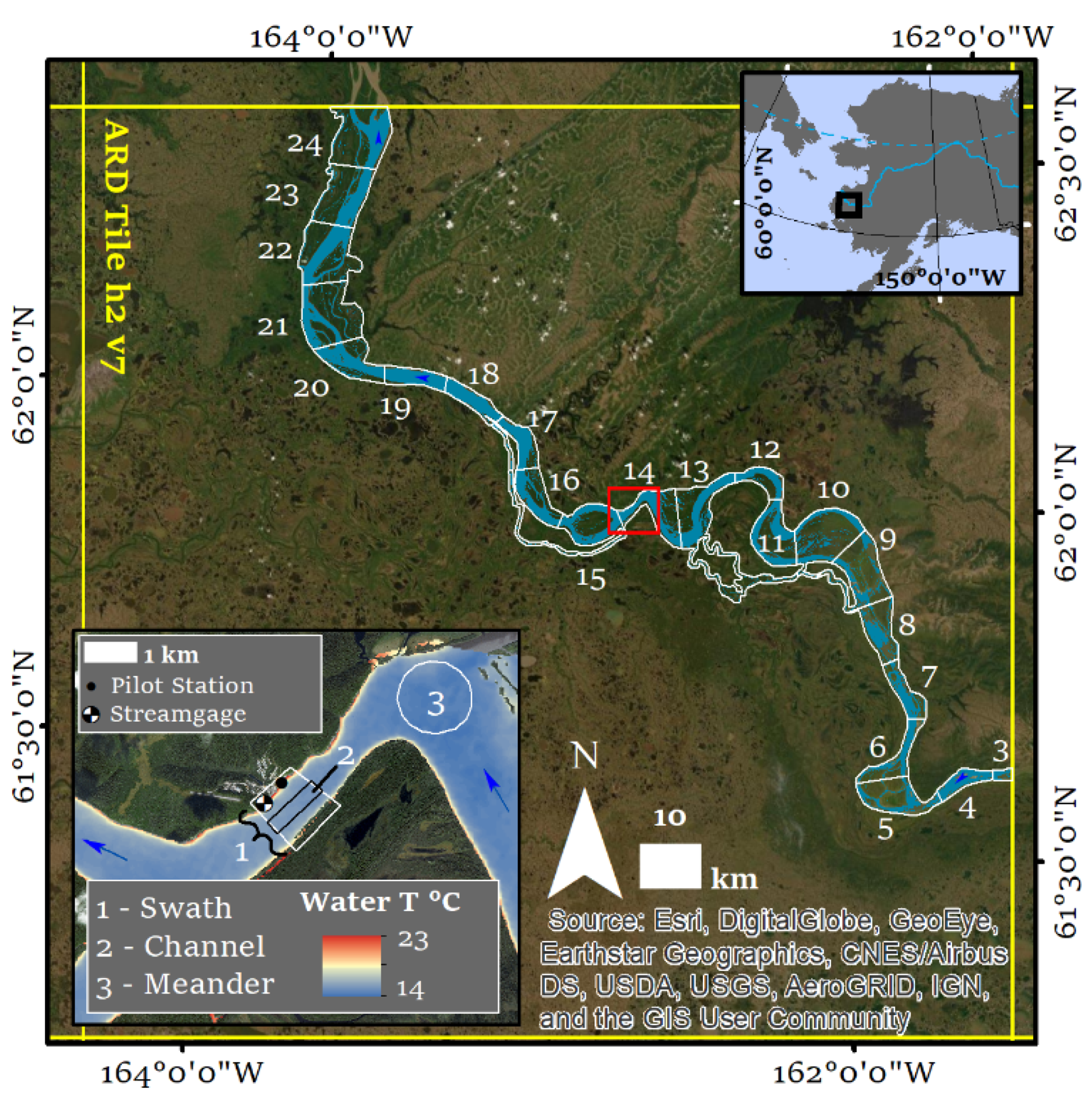
2. Study Area
3. Materials and Methods
4. Results
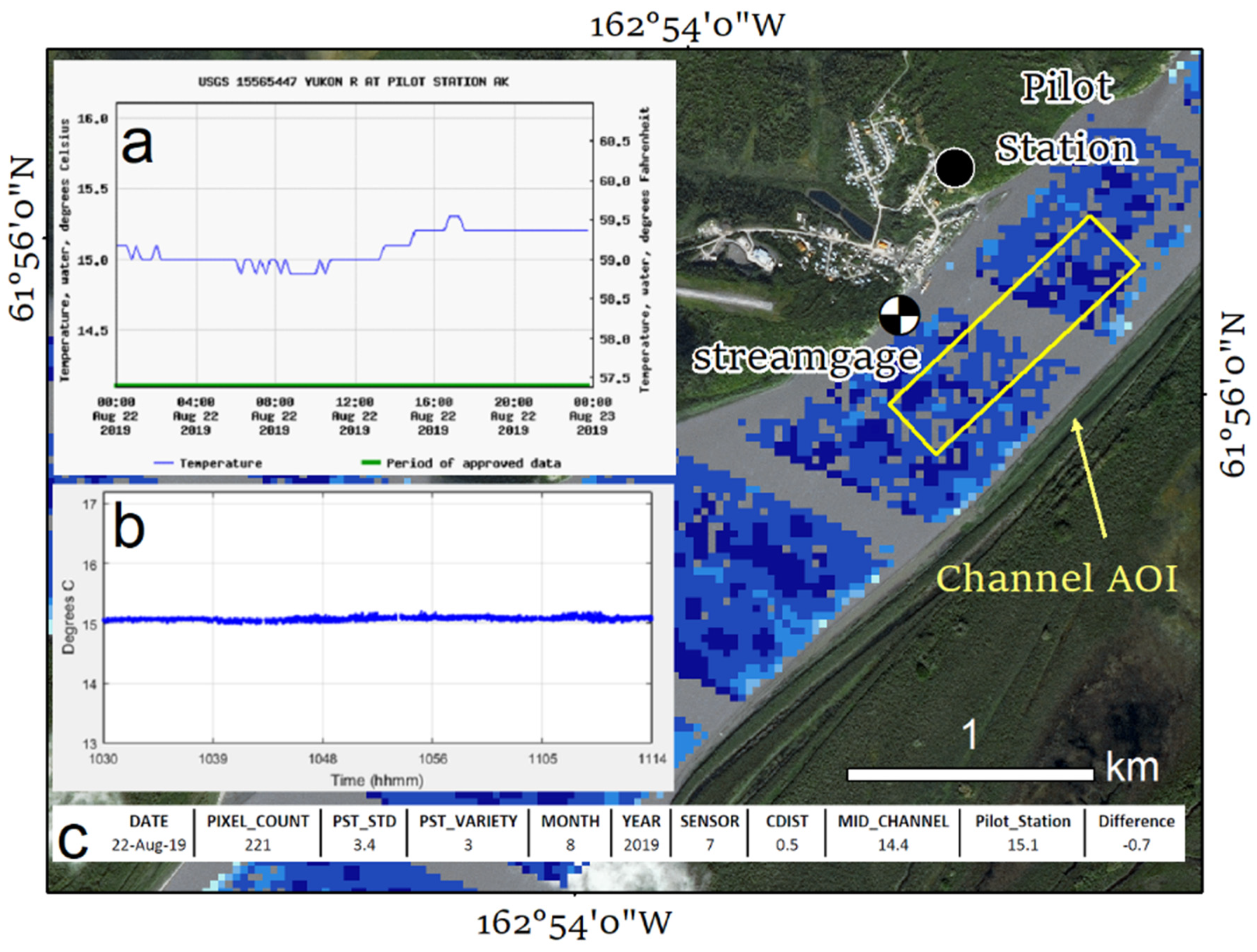
4.1. Provisional Surface Temperature Estimates at the 1 km Scale
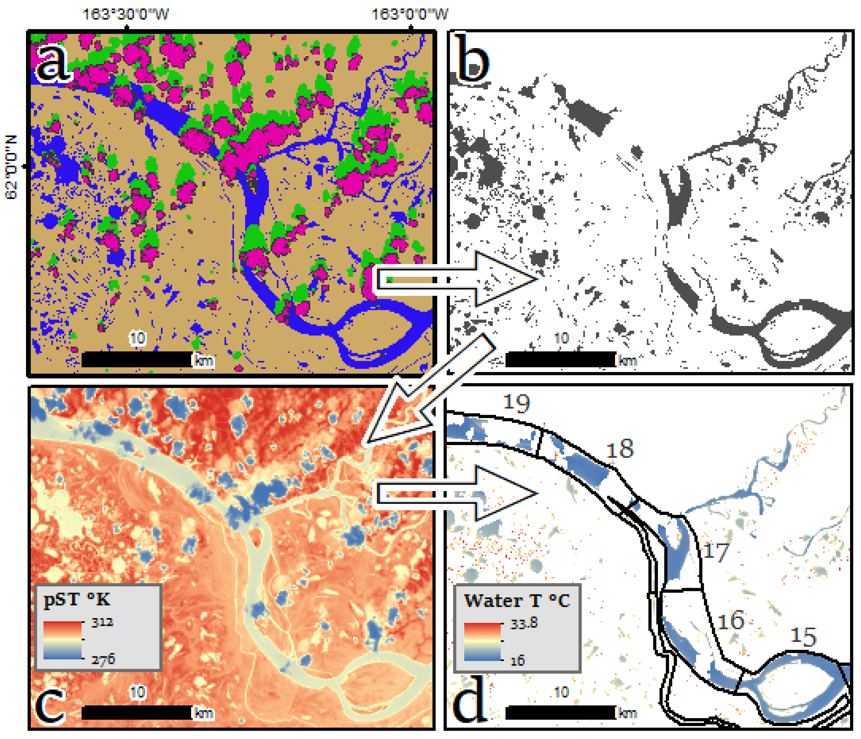
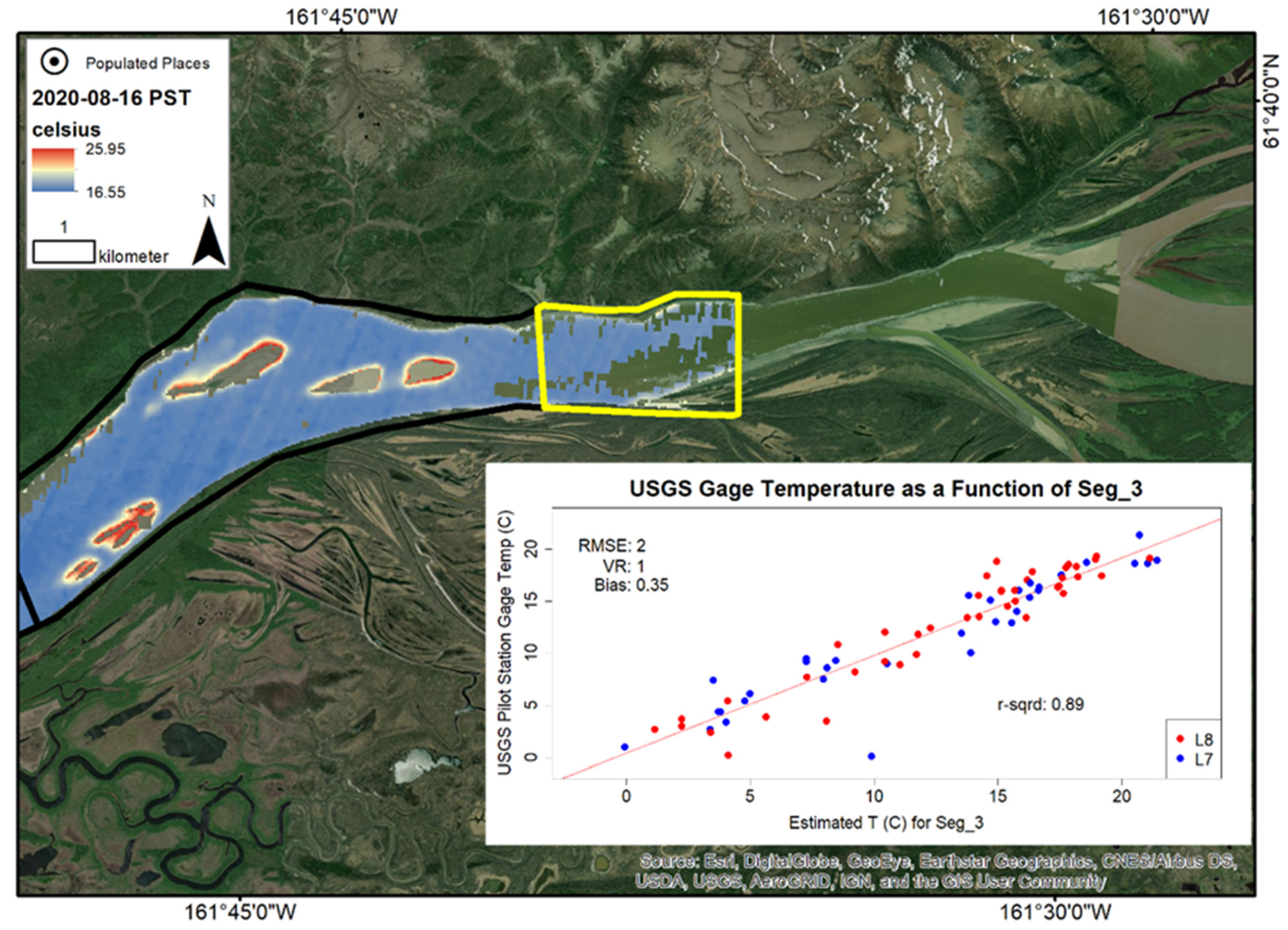
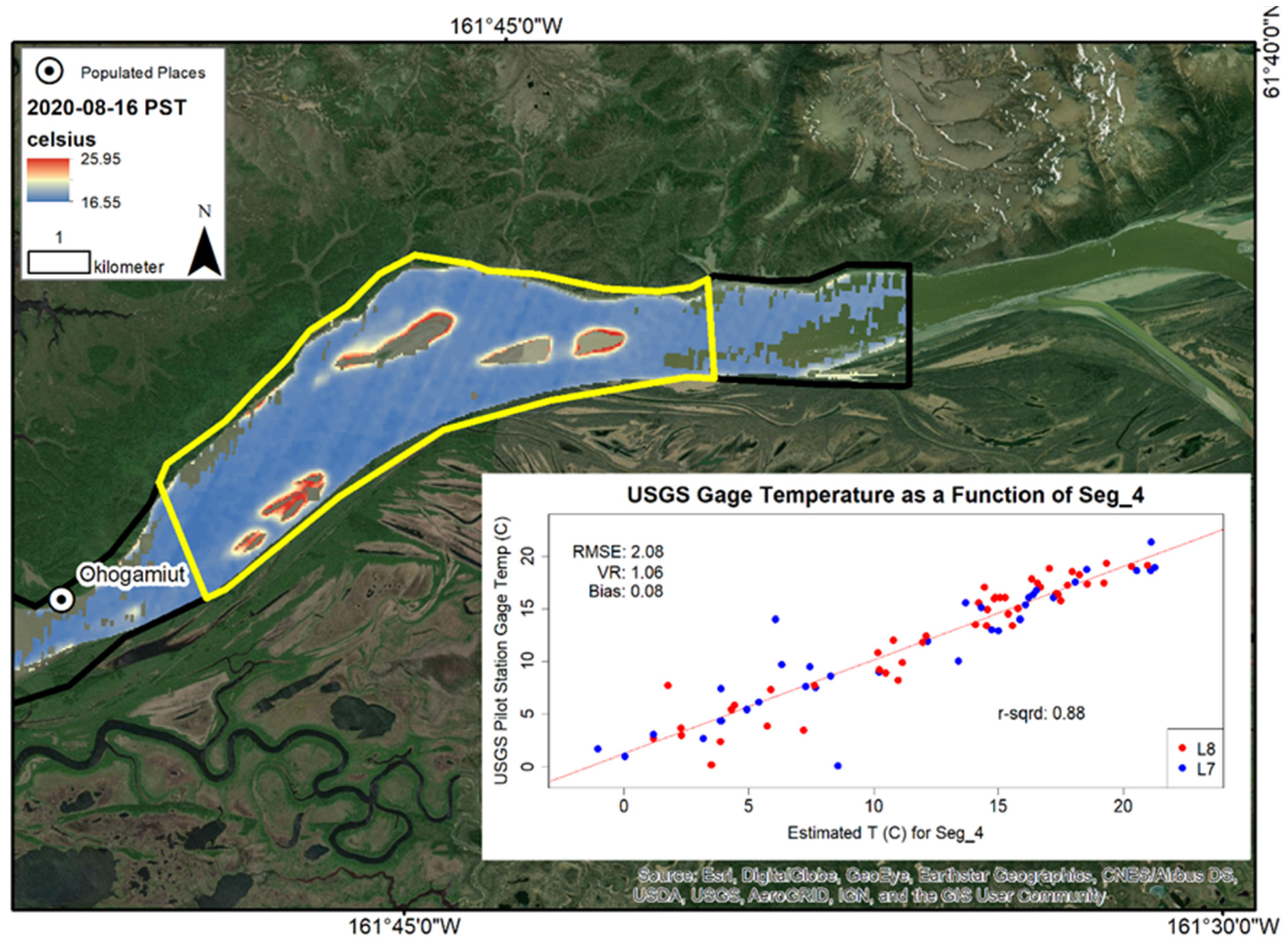
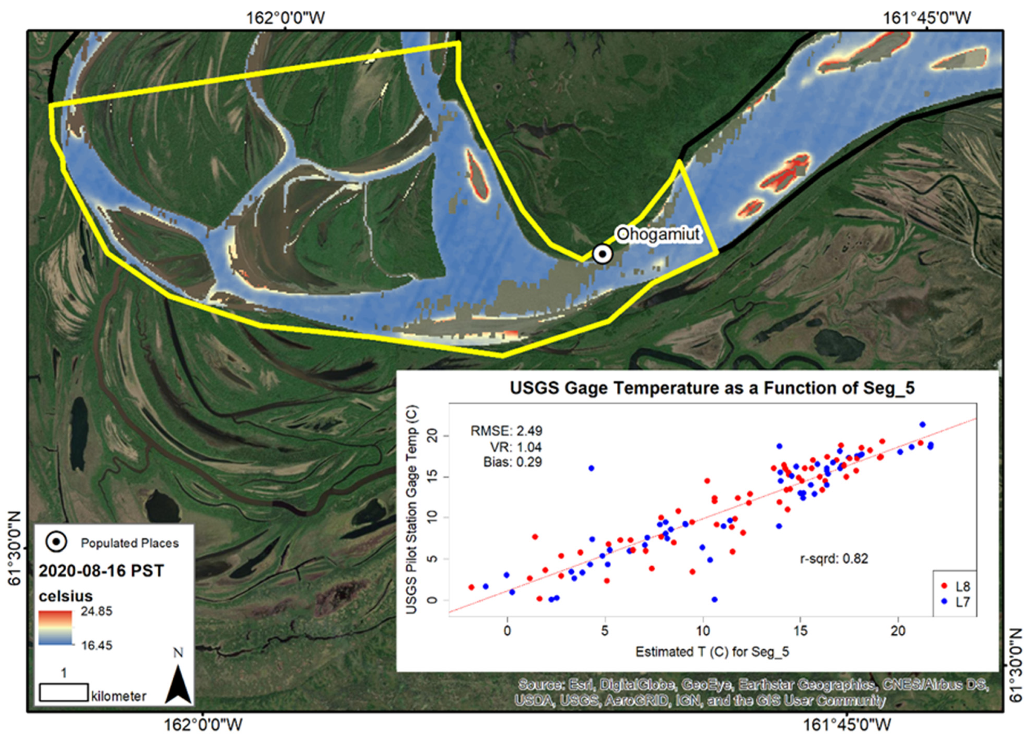
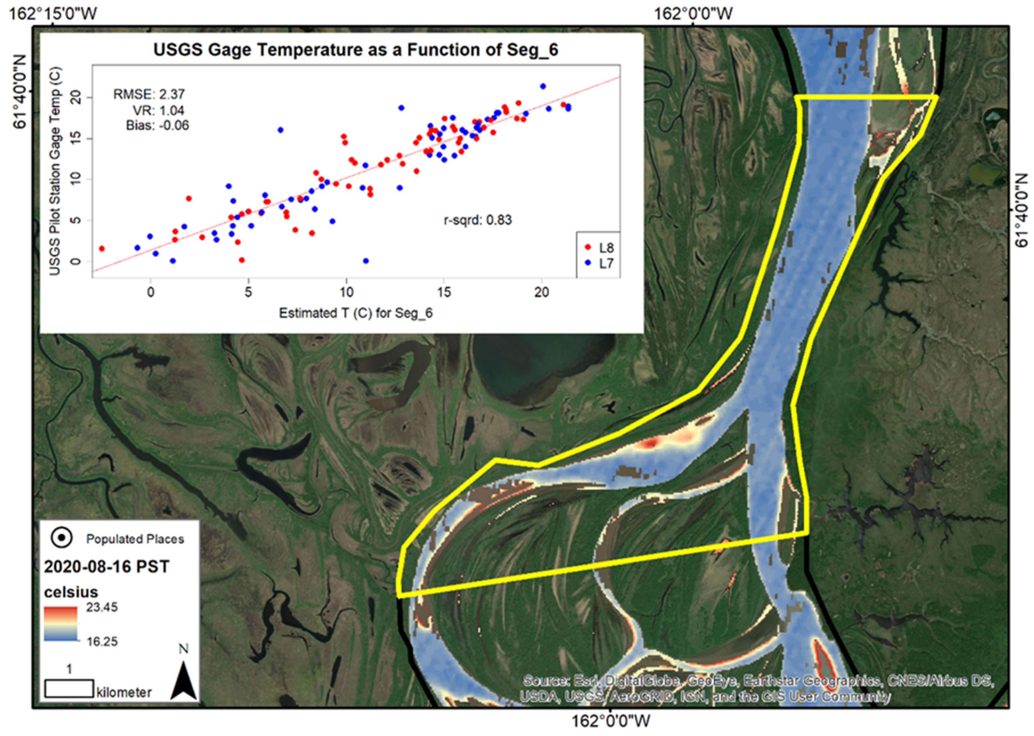
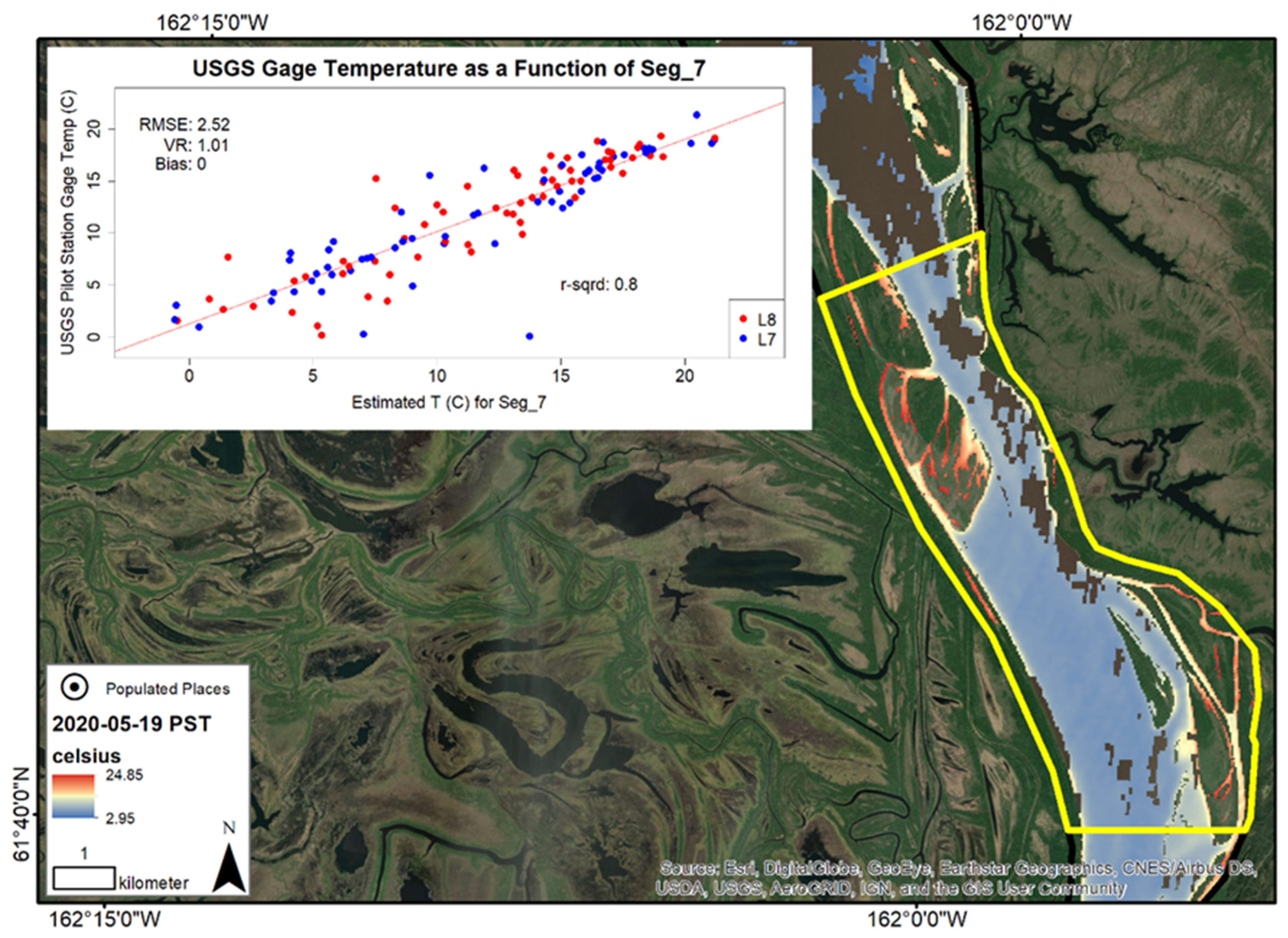
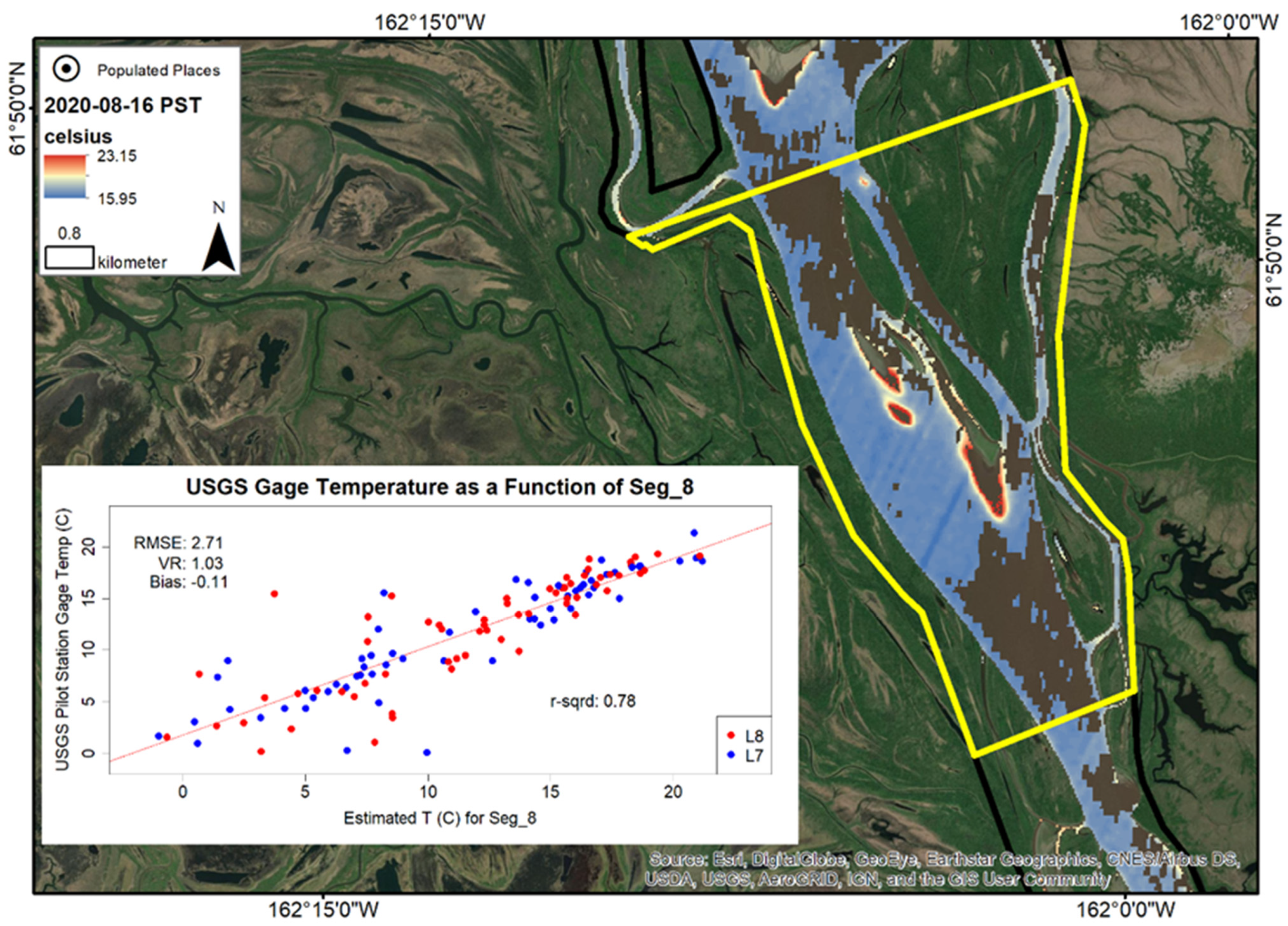
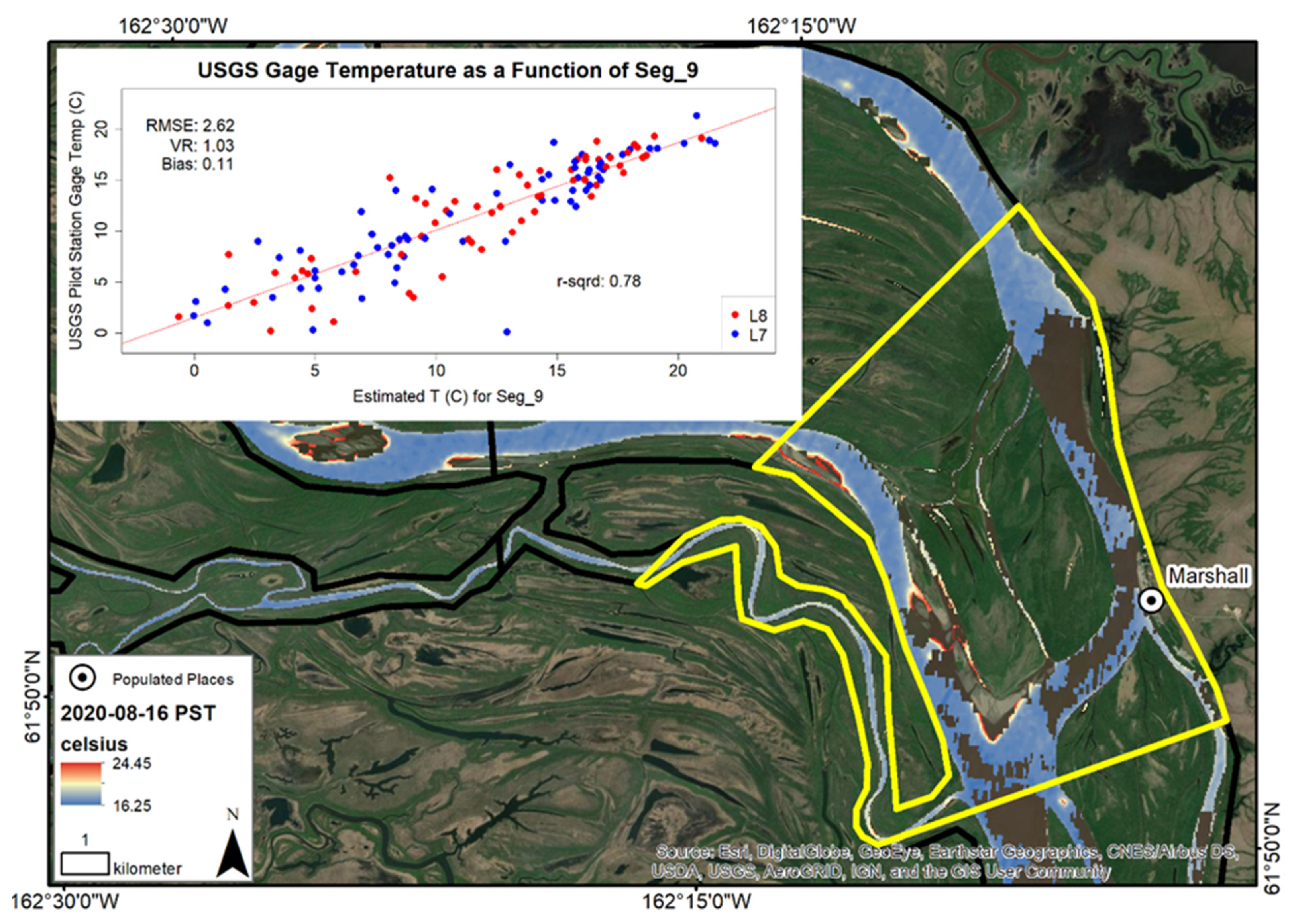
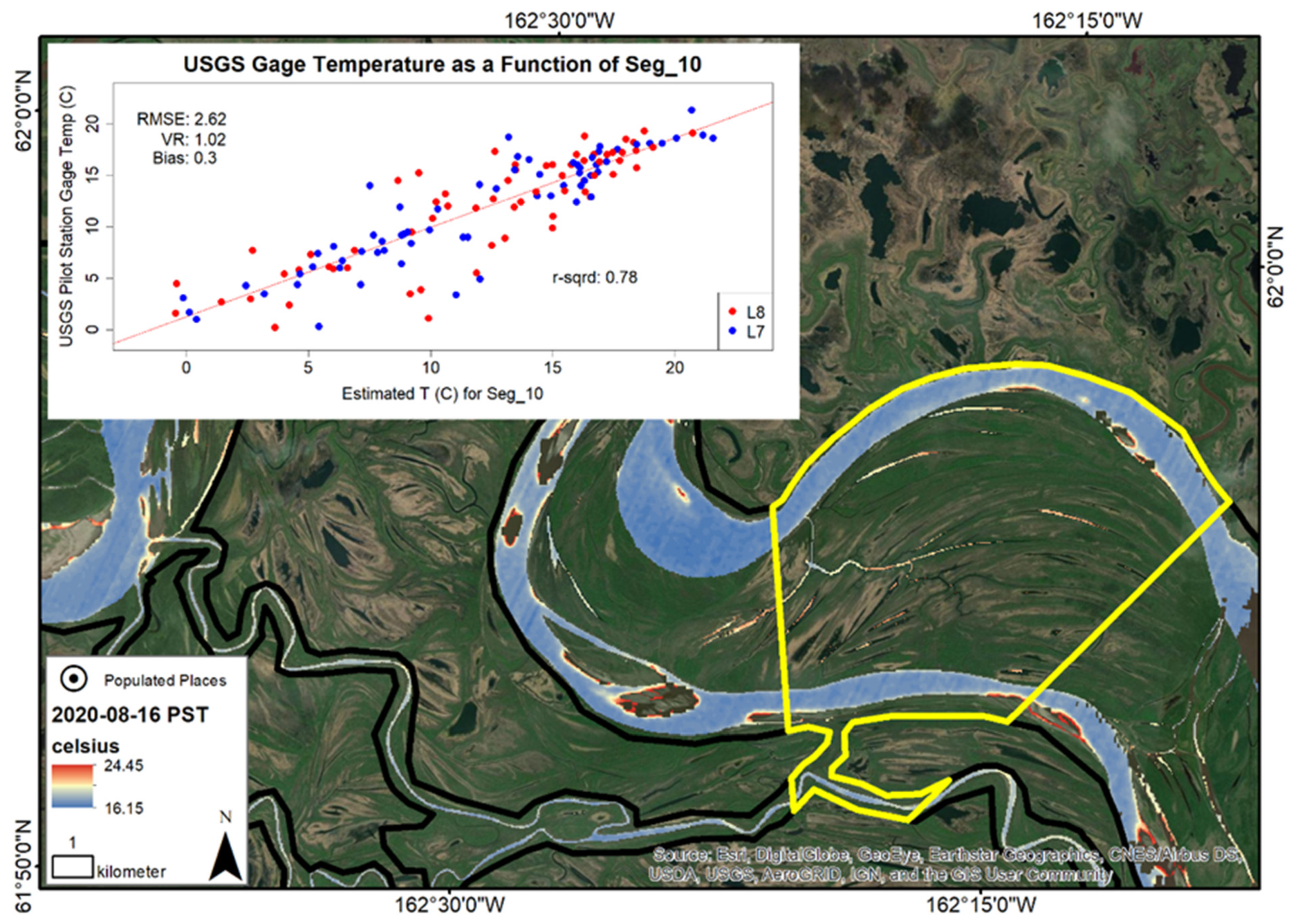
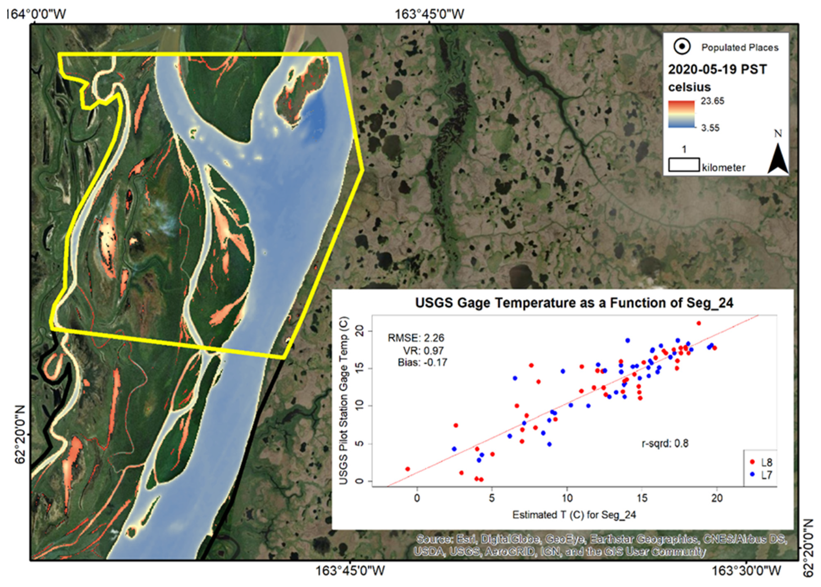
4.2. Provisional Surface Temperature Estimates at the 10 km Scale
4.3. Provisional Surface Temperature Estimates at the 100 km Scale
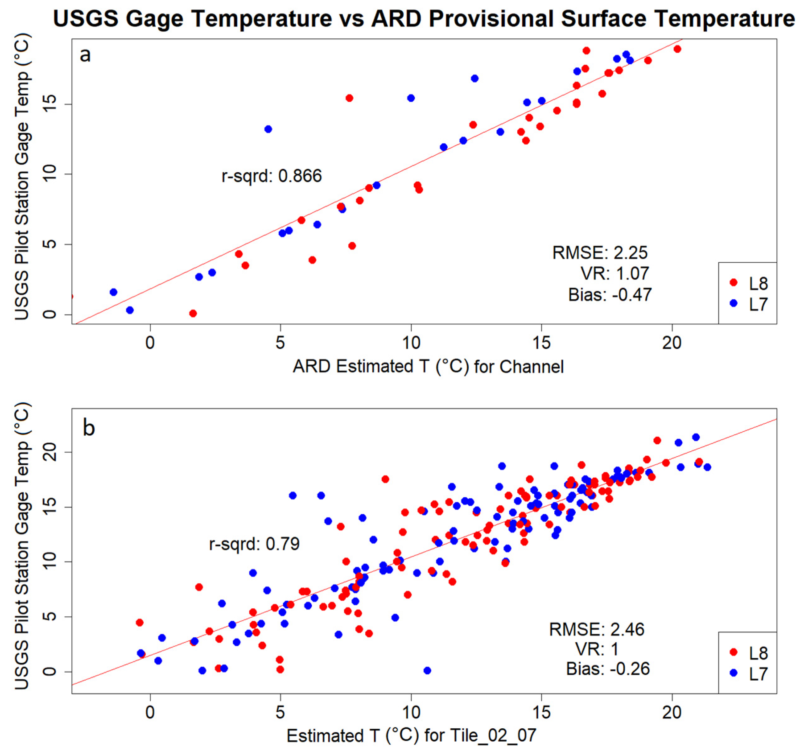
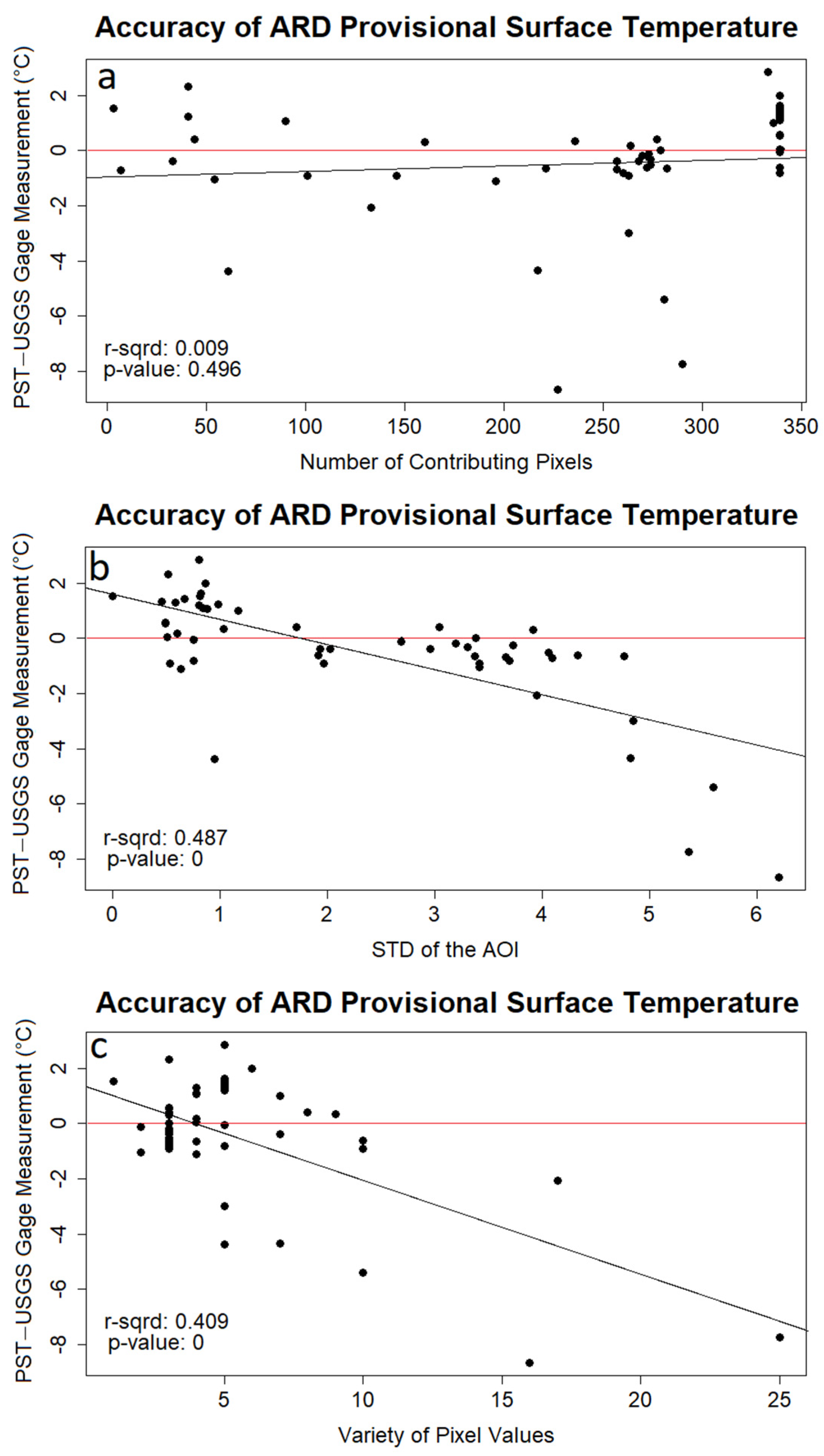
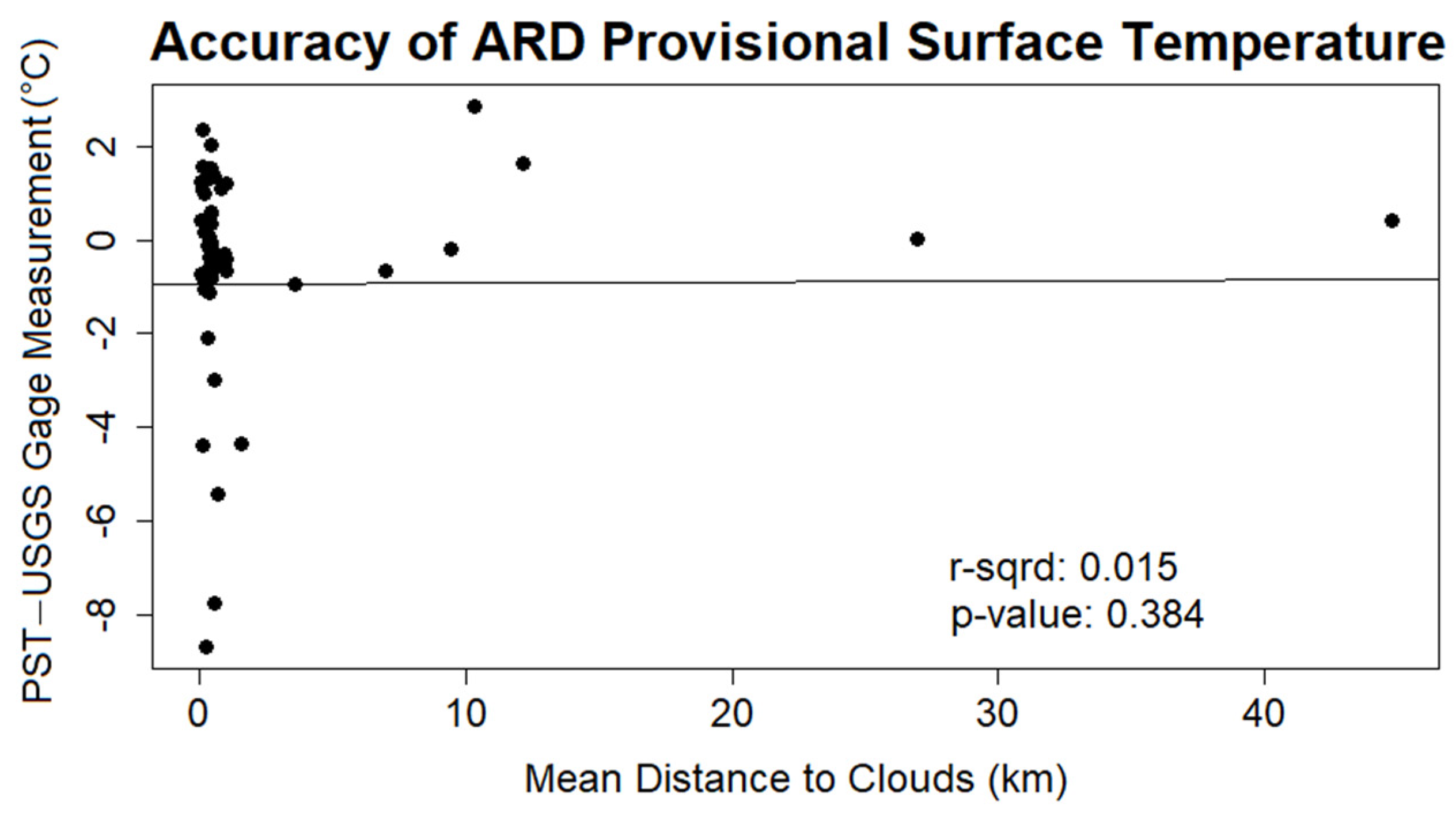
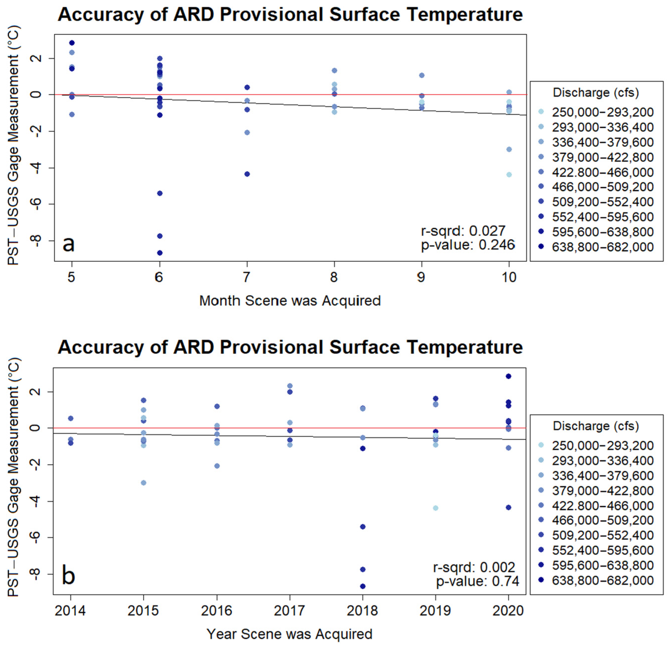
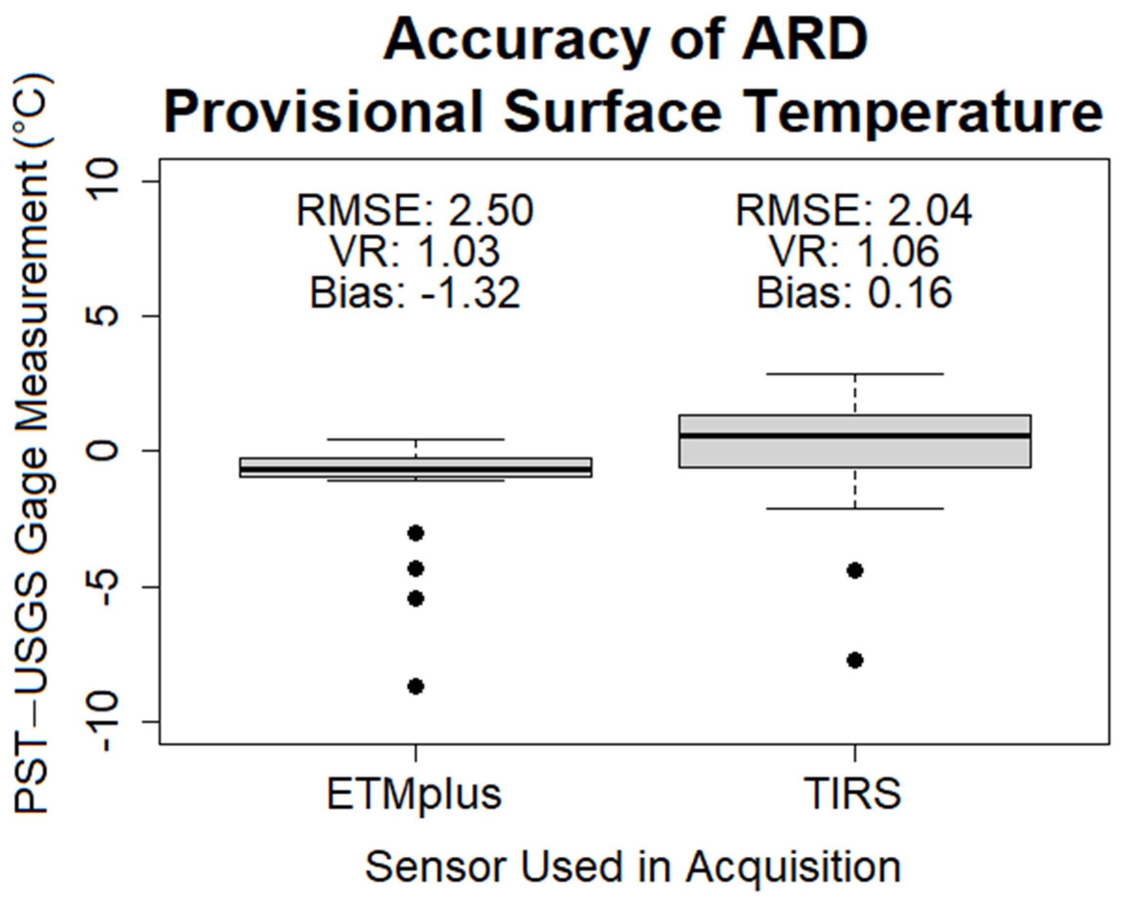
4.4. Error Analysis
5. Discussion
Sources of Error
6. Conclusions
- Landsat ARD provisional surface temperature for the lower Yukon River strongly agrees with in situ water temperature measurements. Approximately 90% of the variation seen within in situ measurements is reflected in remotely sensed estimates.
- Remotely sensed estimates for the Channel AOI adjacent to the Pilot Station streamgage, achieved an RMSE of 2.25 °C compared to in situ measurements.
- For the Yukon River and within our study area, we found similarly good agreement between the Landsat ARD provisional water surface temperature and in situ water temperature measurements taken from areas of interest (AOIs) and river segments distributed upstream or downstream of Pilot Station, Alaska.
- At least in the case of large unstratified rivers in Alaska, ARD pST can be used to infer water temperature at a given point based on immediate and geographically distant river reaches in the event of limited scene availability due to cloud cover, a common problem in northern latitudes.
- pST is downscaled to a 30 m resolution from the original 100 m resolution thermal bands. Optimal agreement between pST estimates and in situ measurements can be found in water bodies where width and/or diameter are much greater than 100 m. Small lakes, narrow sloughs, creeks, and streams, while discernable, are likely to be contaminated by the land surface temperature recorded in adjacent pixels.
- The Yukon river is a large, glacially fed, free flowing river. While it is the largest of such rivers in Alaska it shares many attributes with other large rivers in the state, namely the Tanana, Susitna, Colville, and Copper River. Our analysis suggests that the methods outlined in this study could also be used to augment existing monitoring networks, collect estimates from locations where physical monitoring is impossible, or provide historical estimates from trend analysis.
Author Contributions
Funding
Institutional Review Board Statement
Informed Consent Statement
Data Availability Statement
Acknowledgments
Conflicts of Interest
Appendix A


| Provisional Surface Temperature °C | |||||||||
|---|---|---|---|---|---|---|---|---|---|
| Date | Landsat ARD Product ID | Pixel Count | Area km2 | Min | Max | Range | Mean | STD | USGS Streamgage °C |
| 5/21/2014 | LC08_AK_002007_20140521_20190504_C01_V01 | 4059 | 3.7 | 5.45 | 16.15 | 10.7 | 7.6 | 2.3 | 5.5 |
| 6/4/2014 | LC08_AK_002007_20140604_20190504_C01_V01 | 344,827 | 310.3 | −0.95 | 24.85 | 25.8 | 10.2 | 2.9 | 9 |
| 6/5/2014 | LE07_AK_002007_20140605_20190504_C01_V01 | 1427 | 1.3 | 2.75 | 16.25 | 13.5 | 7.5 | 2.6 | 10 |
| 6/6/2014 | LC08_AK_002007_20140606_20190504_C01_V01 | 4522 | 4.1 | 12.45 | 22.35 | 9.9 | 13.6 | 1.3 | 10 |
| 6/19/2014 | LE07_AK_002007_20140619_20190208_C01_V01 | 141,950 | 127.8 | 11.65 | 23.95 | 12.3 | 13.7 | 1.2 | 13.5 |
| 6/20/2014 | LC08_AK_002007_20140620_20190504_C01_V01 | 389,404 | 350.5 | 13.45 | 29.25 | 15.8 | 15.1 | 1.4 | 14 |
| 6/21/2014 | LE07_AK_002007_20140621_20190504_C01_V01 | 149,300 | 134.4 | 11.65 | 43.05 | 31.4 | 16.1 | 1.8 | 14.5 |
| 6/22/2014 | LC08_AK_002007_20140622_20190504_C01_V01 | 3436 | 3.1 | 14.25 | 29.85 | 15.6 | 16.9 | 2.0 | 15 |
| 6/27/2014 | LC08_AK_002007_20140627_20190504_C01_V01 | 193,873 | 174.5 | 15.75 | 29.35 | 13.6 | 17.0 | 1.0 | 16 |
| 6/30/2014 | LE07_AK_002007_20140630_20190504_C01_V01 | 56,495 | 50.8 | 14.25 | 31.05 | 16.8 | 16.2 | 1.1 | 16 |
| 7/5/2014 | LE07_AK_002007_20140705_20190504_C01_V01 | 138,805 | 124.9 | 13.95 | 37.35 | 23.4 | 16.3 | 1.3 | 17 |
| 7/6/2014 | LC08_AK_002007_20140706_20190504_C01_V01 | 324,732 | 292.3 | 7.65 | 38.95 | 31.3 | 17.7 | 1.5 | 17.5 |
| 7/15/2014 | LC08_AK_002007_20140715_20190208_C01_V01 | 59 | 0.1 | 8.15 | 9.45 | 1.3 | 9.0 | 0.4 | 17.5 |
| 7/29/2014 | LC08_AK_002007_20140729_20190504_C01_V01 | 198,991 | 179.1 | 13.35 | 27.75 | 14.4 | 15.6 | 1.2 | 14.5 |
| 7/30/2014 | LE07_AK_002007_20140730_20190504_C01_V01 | 79,702 | 71.7 | 4.55 | 25.55 | 21 | 12.5 | 2.0 | 14.5 |
| 8/7/2014 | LC08_AK_002007_20140807_20190505_C01_V01 | 1 | 0.001 | 6.55 | 6.55 | 0 | 6.6 | 0.0 | 16 |
| 8/9/2014 | LC08_AK_002007_20140809_20190504_C01_V01 | 5929 | 5.3 | 9.45 | 18.55 | 9.1 | 14.4 | 1.3 | 16 |
| 8/14/2014 | LC08_AK_002007_20140814_20190504_C01_V01 | 36,458 | 32.8 | 8.45 | 22.25 | 13.8 | 16.0 | 1.4 | 17 |
| 8/15/2014 | LE07_AK_002007_20140815_20190504_C01_V01 | 55,910 | 50.3 | 7.45 | 29.35 | 21.9 | 16.9 | 1.6 | 17 |
| 8/16/2014 | LC08_AK_002007_20140816_20190504_C01_V01 | 34,561 | 31.1 | 10.95 | 20.75 | 9.8 | 16.2 | 0.9 | 17 |
| 8/17/2014 | LE07_AK_002007_20140817_20190504_C01_V01 | 5031 | 4.5 | 12.05 | 23.05 | 11 | 16.1 | 1.1 | 17 |
| 8/30/2014 | LC08_AK_002007_20140830_20190504_C01_V01 | 104,275 | 93.8 | 9.95 | 21.05 | 11.1 | 13.9 | 0.6 | 14.5 |
| 8/31/2014 | LE07_AK_002007_20140831_20190503_C01_V01 | 2312 | 2.1 | 5.55 | 13.55 | 8 | 9.8 | 1.3 | 14.5 |
| 9/15/2014 | LC08_AK_002007_20140915_20190504_C01_V01 | 31,264 | 28.1 | 8.25 | 18.95 | 10.7 | 11.1 | 1.9 | 10 |
| 9/16/2014 | LE07_AK_002007_20140916_20190208_C01_V01 | 21,721 | 19.5 | 7.55 | 17.25 | 9.7 | 9.7 | 1.4 | 9.5 |
| 9/18/2014 | LE07_AK_002007_20140918_20181207_C01_V01 | 3306 | 3.0 | 4.75 | 14.65 | 9.9 | 8.2 | 1.2 | 9.5 |
| 10/1/2014 | LC08_AK_002007_20141001_20190503_C01_V01 | 164,602 | 148.1 | 6.25 | 13.95 | 7.7 | 7.5 | 0.8 | 7.1 |
| 10/3/2014 | LC08_AK_002007_20141003_20190503_C01_V01 | 167,863 | 151.1 | 1.95 | 10.85 | 8.9 | 5.2 | 0.5 | 6.1 |
| 10/4/2014 | LE07_AK_002007_20141004_20190503_C01_V01 | 33,394 | 30.1 | −2.45 | 9.15 | 11.6 | 4.0 | 1.1 | 5.4 |
| 5/15/2015 | LC08_AK_002007_20150515_20190502_C01_V01 | 8886 | 8.0 | −6.05 | 17.05 | 23.1 | 2.0 | 3.1 | 0.1 |
| 5/24/2015 | LC08_AK_002007_20150524_20190607_C01_V01 | 3319 | 3.0 | 3.05 | 16.75 | 13.7 | 6.7 | 1.4 | 5.9 |
| 5/29/2015 | LC08_AK_002007_20150529_20190502_C01_V01 | 38,728 | 34.9 | 4.35 | 22.45 | 18.1 | 9.6 | 3.0 | 10.1 |
| 5/30/2015 | LE07_AK_002007_20150530_20190208_C01_V01 | 183,585 | 165.2 | 7.95 | 33.35 | 25.4 | 13.2 | 2.3 | 11 |
| 5/31/2015 | LC08_AK_002007_20150531_20190502_C01_V01 | 18,948 | 17.1 | 2.65 | 20.95 | 18.3 | 11.7 | 2.2 | 11.9 |
| 6/1/2015 | LE07_AK_002007_20150601_20181206_C01_V01 | 8362 | 7.5 | 4.15 | 17.15 | 13 | 9.7 | 1.7 | 12.7 |
| 6/6/2015 | LE07_AK_002007_20150606_20190502_C01_V01 | 653 | 0.6 | 4.45 | 10.45 | 6 | 6.8 | 1.0 | 13.7 |
| 6/14/2015 | LC08_AK_002007_20150614_20190502_C01_V01 | 203,896 | 183.5 | 12.85 | 24.55 | 11.7 | 14.3 | 1.2 | 12.6 |
| 6/15/2015 | LE07_AK_002007_20150615_20190502_C01_V01 | 335,071 | 301.6 | 11.25 | 25.25 | 14 | 13.9 | 1.4 | 13 |
| 6/16/2015 | LC08_AK_002007_20150616_20190502_C01_V01 | 329,362 | 296.4 | 8.85 | 26.85 | 18 | 15.3 | 1.7 | 13.4 |
| 6/17/2015 | LE07_AK_002007_20150617_20181206_C01_V01 | 90,172 | 81.2 | 13.75 | 30.15 | 16.4 | 16.1 | 1.8 | 14 |
| 6/22/2015 | LE07_AK_002007_20150622_20190502_C01_V01 | 80,318 | 72.3 | 5.85 | 25.45 | 19.6 | 14.6 | 3.1 | 17.5 |
| 6/23/2015 | LC08_AK_002007_20150623_20190502_C01_V01 | 211,305 | 190.2 | 9.85 | 30.85 | 21 | 19.1 | 0.9 | 18.1 |
| 6/24/2015 | LE07_AK_002007_20150624_20190502_C01_V01 | 182,729 | 164.5 | 16.35 | 29.35 | 13 | 18.4 | 0.9 | 18.5 |
| 6/25/2015 | LC08_AK_002007_20150625_20190502_C01_V01 | 108,263 | 97.4 | 19.25 | 29.05 | 9.8 | 20.3 | 0.8 | 18.6 |
| 7/27/2015 | LC08_AK_002007_20150727_20190501_C01_V01 | 1788 | 1.6 | 15.85 | 23.55 | 7.7 | 17.3 | 0.9 | 16.4 |
| 8/2/2015 | LE07_AK_002007_20150802_20190501_C01_V01 | 132,993 | 119.7 | 12.75 | 30.05 | 17.3 | 16.8 | 1.0 | 17.3 |
| 8/3/2015 | LC08_AK_002007_20150803_20190501_C01_V01 | 251,387 | 226.2 | 15.75 | 30.05 | 14.3 | 18.4 | 0.8 | 17.4 |
| 8/4/2015 | LE07_AK_002007_20150804_20181206_C01_V01 | 75,918 | 68.3 | 16.25 | 31.35 | 15.1 | 17.8 | 1.0 | 17.5 |
| 9/11/2015 | LC08_AK_002007_20150911_20190501_C01_V01 | 83,123 | 74.8 | 3.15 | 12.25 | 9.1 | 9.5 | 0.7 | 10 |
| 9/20/2015 | LC08_AK_002007_20150920_20190501_C01_V01 | 95,783 | 86.2 | 3.45 | 12.15 | 8.7 | 7.1 | 0.7 | 7.6 |
| 9/21/2015 | LE07_AK_002007_20150921_20190501_C01_V01 | 11,730 | 10.6 | 3.05 | 12.45 | 9.4 | 5.9 | 0.8 | 7.3 |
| 9/26/2015 | LE07_AK_002007_20150926_20190501_C01_V01 | 55,449 | 49.9 | 0.25 | 7.95 | 7.7 | 2.8 | 0.8 | 6.2 |
| 9/28/2015 | LE07_AK_002007_20150928_20190501_C01_V01 | 60,172 | 54.2 | −7.55 | 8.15 | 15.7 | 4.8 | 0.7 | 5.8 |
| 9/29/2015 | LC08_AK_002007_20150929_20190501_C01_V01 | 15,436 | 13.9 | 1.95 | 7.95 | 6 | 5.1 | 0.5 | 5.4 |
| 10/5/2015 | LE07_AK_002007_20151005_20190207_C01_V01 | 6 | 0.005 | −1.15 | 0.35 | 1.5 | −0.4 | 0.4 | 4.5 |
| 10/7/2015 | LE07_AK_002007_20151007_20181206_C01_V01 | 70,323 | 63.3 | 2.05 | 11.05 | 9 | 4.3 | 1.2 | 4.4 |
| 10/14/2015 | LE07_AK_002007_20151014_20190501_C01_V01 | 163,062 | 146.8 | 0.15 | 11.85 | 11.7 | 2.7 | 1.0 | 3 |
| 10/15/2015 | LC08_AK_002007_20151015_20190501_C01_V01 | 46,883 | 42.2 | 2.25 | 8.75 | 6.5 | 3.3 | 0.6 | 2.7 |
| 10/21/2015 | LE07_AK_002007_20151021_20190501_C01_V01 | 103,946 | 93.6 | −3.45 | 3.45 | 6.9 | −0.3 | 0.9 | 1.6 |
| 10/23/2015 | LE07_AK_002007_20151023_20181210_C01_V01 | 70,903 | 63.8 | −1.35 | 5.65 | 7 | 0.3 | 0.8 | 1 |
| 5/15/2016 | LC08_AK_002007_20160515_20190430_C01_V01 | 182,934 | 164.6 | 3.15 | 24.85 | 21.7 | 8.0 | 2.6 | 5.3 |
| 5/16/2016 | LE07_AK_002007_20160516_20181211_C01_V01 | 330,368 | 297.3 | 1.45 | 28.85 | 27.4 | 7.9 | 3.0 | 6.4 |
| 5/17/2016 | LC08_AK_002007_20160517_20190430_C01_V01 | 19,028 | 17.1 | −0.85 | 26.95 | 27.8 | 9.9 | 3.8 | 7 |
| 5/26/2016 | LC08_AK_002007_20160526_20190607_C01_V01 | 134,738 | 121.3 | 5.85 | 23.05 | 17.2 | 10.9 | 1.3 | 9 |
| 5/31/2016 | LC08_AK_002007_20160531_20190430_C01_V01 | 208,830 | 187.9 | 12.35 | 30.55 | 18.2 | 14.3 | 2.0 | 11.8 |
| 6/2/2016 | LC08_AK_002007_20160602_20181211_C01_V01 | 336,772 | 303.1 | 12.65 | 28.35 | 15.7 | 14.5 | 1.3 | 13 |
| 6/16/2016 | LC08_AK_002007_20160616_20190430_C01_V01 | 47,095 | 42.4 | 3.05 | 24.25 | 21.2 | 11.1 | 3.2 | 14.6 |
| 7/2/2016 | LC08_AK_002007_20160702_20181210_C01_V01 | 24,564 | 22.1 | 6.75 | 24.05 | 17.3 | 13.5 | 2.4 | 18.7 |
| 7/4/2016 | LC08_AK_002007_20160704_20181211_C01_V01 | 153,688 | 138.3 | 5.55 | 28.95 | 23.4 | 16.5 | 2.2 | 18.8 |
| 7/10/2016 | LE07_AK_002007_20160710_20190430_C01_V01 | 121,659 | 109.5 | 15.05 | 24.65 | 9.6 | 17.9 | 0.7 | 18.3 |
| 7/12/2016 | LE07_AK_002007_20160712_20181209_C01_V01 | 237,587 | 213.8 | 16.15 | 33.95 | 17.8 | 18.4 | 1.3 | 18.2 |
| 7/13/2016 | LC08_AK_002007_20160713_20190430_C01_V01 | 110,388 | 99.3 | 19.75 | 36.35 | 16.6 | 21.4 | 1.4 | 18.6 |
| 7/26/2016 | LE07_AK_002007_20160726_20190430_C01_V01 | 124,632 | 112.2 | 11.25 | 30.45 | 19.2 | 17.0 | 1.5 | 17.3 |
| 8/4/2016 | LE07_AK_002007_20160804_20190430_C01_V01 | 13,625 | 12.3 | 7.85 | 25.15 | 17.3 | 14.9 | 2.0 | 16 |
| 8/6/2016 | LE07_AK_002007_20160806_20181201_C01_V01 | 14,425 | 13.0 | 13.95 | 21.15 | 7.2 | 15.6 | 0.5 | 16 |
| 8/12/2016 | LC08_AK_002007_20160812_20190430_C01_V01 | 3016 | 2.7 | 10.05 | 18.85 | 8.8 | 12.1 | 1.1 | 15.5 |
| 8/14/2016 | LC08_AK_002007_20160814_20190430_C01_V01 | 10,291 | 9.3 | 9.65 | 18.75 | 9.1 | 13.7 | 1.7 | 16 |
| 8/22/2016 | LE07_AK_002007_20160822_20181201_C01_V01 | 6651 | 6.0 | 11.45 | 21.85 | 10.4 | 15.5 | 0.8 | 16.2 |
| 8/27/2016 | LE07_AK_002007_20160827_20190430_C01_V01 | 29,565 | 26.6 | 9.15 | 20.15 | 11 | 14.4 | 1.2 | 15.8 |
| 8/28/2016 | LC08_AK_002007_20160828_20190430_C01_V01 | 82,705 | 74.4 | 14.25 | 21.35 | 7.1 | 16.1 | 0.5 | 15.7 |
| 8/29/2016 | LE07_AK_002007_20160829_20190207_C01_V01 | 53,225 | 47.9 | 4.65 | 20.55 | 15.9 | 14.1 | 1.5 | 15.5 |
| 8/30/2016 | LC08_AK_002007_20160830_20190430_C01_V01 | 138,824 | 124.9 | 15.55 | 22.35 | 6.8 | 16.5 | 0.6 | 15.3 |
| 9/5/2016 | LE07_AK_002007_20160905_20181201_C01_V01 | 42,719 | 38.4 | 7.25 | 20.55 | 13.3 | 13.4 | 0.9 | 14.8 |
| 9/7/2016 | LE07_AK_002007_20160907_20181204_C01_V01 | 21,415 | 19.3 | 7.05 | 16.65 | 9.6 | 13.3 | 0.9 | 14.1 |
| 9/30/2016 | LE07_AK_002007_20160930_20181201_C01_V01 | 2566 | 2.3 | 4.45 | 11.55 | 7.1 | 6.0 | 1.3 | 7.3 |
| 10/7/2016 | LE07_AK_002007_20161007_20181209_C01_V01 | 335,109 | 301.6 | 3.75 | 11.85 | 8.1 | 6.1 | 1.1 | 6 |
| 10/14/2016 | LE07_AK_002007_20161014_20181209_C01_V01 | 83,959 | 75.6 | 0.55 | 10.05 | 9.5 | 4.0 | 0.4 | 4.3 |
| 10/15/2016 | LC08_AK_002007_20161015_20190607_C01_V01 | 212,929 | 191.6 | 0.95 | 7.85 | 6.9 | 3.8 | 0.5 | 3.5 |
| 10/16/2016 | LE07_AK_002007_20161016_20181201_C01_V01 | 226,172 | 203.6 | −2.45 | 7.45 | 9.9 | 1.7 | 0.6 | 2.7 |
| 10/17/2016 | LC08_AK_002007_20161017_20190430_C01_V01 | 63,734 | 57.4 | −5.25 | 2.15 | 7.4 | −0.4 | 0.9 | 1.7 |
| 5/20/2017 | LC08_AK_002007_20170520_20181127_C01_V01 | 139,940 | 125.9 | 1.55 | 31.45 | 29.9 | 8.0 | 3.7 | 3.9 |
| 5/21/2017 | LE07_AK_002007_20170521_20181127_C01_V01 | 64,264 | 57.8 | 1.75 | 28.05 | 26.3 | 5.2 | 3.4 | 4.4 |
| 5/27/2017 | LC08_AK_002007_20170527_20190430_C01_V01 | 30,030 | 27.0 | −0.55 | 18.85 | 19.4 | 7.4 | 1.8 | 6.8 |
| 5/28/2017 | LE07_AK_002007_20170528_20181209_C01_V01 | 45,387 | 40.8 | 2.85 | 19.05 | 16.2 | 7.9 | 1.5 | 7.5 |
| 5/29/2017 | LC08_AK_002007_20170529_20190430_C01_V01 | 82,747 | 74.5 | 4.35 | 27.75 | 23.4 | 11.6 | 2.5 | 8.2 |
| 6/3/2017 | LC08_AK_002007_20170603_20181204_C01_V01 | 191,980 | 172.8 | 10.45 | 31.15 | 20.7 | 13.7 | 2.3 | 11.2 |
| 6/4/2017 | LE07_AK_002007_20170604_20181209_C01_V01 | 310,146 | 279.1 | 6.85 | 36.05 | 29.2 | 12.9 | 2.5 | 11.9 |
| 6/5/2017 | LC08_AK_002007_20170605_20181204_C01_V01 | 265,737 | 239.2 | 10.15 | 35.05 | 24.9 | 15.5 | 2.5 | 12.4 |
| 6/6/2017 | LE07_AK_002007_20170606_20181209_C01_V01 | 1448 | 1.3 | 9.65 | 18.35 | 8.7 | 12.9 | 1.7 | 12.9 |
| 6/11/2017 | LE07_AK_002007_20170611_20190430_C01_V01 | 2 | 0.002 | 10.65 | 12.85 | 2.2 | 11.8 | 1.1 | 15.1 |
| 6/12/2017 | LC08_AK_002007_20170612_20190430_C01_V01 | 10,069 | 9.1 | 6.95 | 18.25 | 11.3 | 10.9 | 2.1 | 15.2 |
| 6/22/2017 | LE07_AK_002007_20170622_20181127_C01_V01 | 26 | 0.023 | 3.25 | 8.15 | 4.9 | 5.5 | 1.3 | 16 |
| 8/6/2017 | LC08_AK_002007_20170806_20181203_C01_V01 | 153,828 | 138.4 | 16.55 | 30.05 | 13.5 | 19.2 | 1.4 | 17.7 |
| 8/7/2017 | LE07_AK_002007_20170807_20181204_C01_V01 | 137,312 | 123.6 | 14.35 | 35.15 | 20.8 | 18.6 | 1.6 | 18.1 |
| 8/17/2017 | LC08_AK_002007_20170817_20190430_C01_V01 | 40,004 | 36.0 | 10.75 | 23.15 | 12.4 | 17.5 | 0.9 | 16.4 |
| 8/23/2017 | LE07_AK_002007_20170823_20181130_C01_V01 | 879 | 0.8 | 7.65 | 12.65 | 5 | 10.5 | 1.0 | 14.6 |
| 8/31/2017 | LC08_AK_002007_20170831_20190430_C01_V01 | 16,753 | 15.1 | 4.05 | 15.55 | 11.5 | 11.5 | 1.1 | 12.4 |
| 9/26/2017 | LE07_AK_002007_20170926_20181130_C01_V01 | 88,872 | 80.0 | 5.95 | 14.25 | 8.3 | 8.2 | 0.7 | 8.6 |
| 10/12/2017 | LE07_AK_002007_20171012_20181121_C01_V01 | 9681 | 8.7 | 3.85 | 11.15 | 7.3 | 7.0 | 1.5 | 6 |
| 10/18/2017 | LC08_AK_002007_20171018_20190430_C01_V01 | 140,868 | 126.8 | −2.15 | 5.85 | 8 | 3.2 | 1.0 | 4.3 |
| 10/19/2017 | LE07_AK_002007_20171019_20181130_C01_V01 | 92,923 | 83.6 | −3.65 | 7.15 | 10.8 | 2.3 | 1.0 | 3.7 |
| 10/20/2017 | LC08_AK_002007_20171020_20190430_C01_V01 | 26,125 | 23.5 | −3.65 | 2.85 | 6.5 | 0.5 | 1.1 | 3.1 |
| 5/23/2018 | LC08_AK_002007_20180523_20190615_C01_V01 | 135,115 | 121.6 | 3.95 | 28.35 | 24.4 | 8.4 | 3.7 | 3.5 |
| 5/31/2018 | LE07_AK_002007_20180531_20190615_C01_V01 | 21,157 | 19.0 | 2.95 | 18.85 | 15.9 | 7.9 | 1.6 | 9.2 |
| 6/1/2018 | LC08_AK_002007_20180601_20190615_C01_V01 | 12,707 | 11.4 | 8.35 | 23.55 | 15.2 | 13.6 | 2.9 | 9.9 |
| 6/6/2018 | LC08_AK_002007_20180606_20190615_C01_V01 | 207,676 | 186.9 | 4.35 | 23.85 | 19.5 | 11.6 | 2.3 | 12.8 |
| 6/7/2018 | LE07_AK_002007_20180607_20190615_C01_V01 | 281,730 | 253.6 | 0.85 | 17.85 | 17 | 7.3 | 2.1 | 13.2 |
| 6/8/2018 | LC08_AK_002007_20180608_20190617_C01_V01 | 55,907 | 50.3 | 12.05 | 21.05 | 9 | 13.9 | 0.8 | 13.5 |
| 6/9/2018 | LE07_AK_002007_20180609_20190615_C01_V01 | 120,285 | 108.3 | 12.05 | 23.25 | 11.2 | 14.4 | 1.1 | 13.5 |
| 6/14/2018 | LE07_AK_002007_20180614_20190615_C01_V01 | 143,239 | 128.9 | 13.25 | 25.15 | 11.9 | 14.8 | 0.7 | 15.3 |
| 6/15/2018 | LC08_AK_002007_20180615_20190615_C01_V01 | 74,902 | 67.4 | 1.75 | 19.45 | 17.7 | 11.5 | 2.6 | 15.4 |
| 6/16/2018 | LE07_AK_002007_20180616_20190615_C01_V01 | 61,190 | 55.1 | 4.45 | 20.95 | 16.5 | 12.3 | 2.0 | 15.4 |
| 6/22/2018 | LC08_AK_002007_20180622_20190615_C01_V01 | 11,085 | 10.0 | 10.85 | 18.45 | 7.6 | 14.3 | 0.9 | 14.2 |
| 6/24/2018 | LC08_AK_002007_20180624_20190615_C01_V01 | 99,964 | 90.0 | 10.95 | 25.85 | 14.9 | 16.2 | 1.3 | 14.5 |
| 6/25/2018 | LE07_AK_002007_20180625_20190615_C01_V01 | 12,578 | 11.3 | 12.15 | 23.55 | 11.4 | 14.8 | 1.1 | 14.9 |
| 7/1/2018 | LC08_AK_002007_20180701_20190615_C01_V01 | 23,655 | 21.3 | 11.15 | 19.95 | 8.8 | 14.7 | 1.3 | 16.5 |
| 7/3/2018 | LC08_AK_002007_20180703_20190615_C01_V01 | 86,642 | 78.0 | 0.95 | 28.75 | 27.8 | 18.4 | 1.8 | 17.3 |
| 7/25/2018 | LE07_AK_002007_20180725_20190614_C01_V01 | 121,860 | 109.7 | 13.05 | 34.65 | 21.6 | 18.3 | 1.9 | 18 |
| 7/26/2018 | LC08_AK_002007_20180726_20190614_C01_V01 | 9522 | 8.6 | 13.95 | 25.35 | 11.4 | 18.8 | 1.1 | 18.3 |
| 9/10/2018 | LC08_AK_002007_20180910_20190614_C01_V01 | 191,059 | 172.0 | 11.35 | 20.75 | 9.4 | 12.4 | 0.9 | 11.2 |
| 9/13/2018 | LE07_AK_002007_20180913_20190614_C01_V01 | 47,697 | 42.9 | 3.55 | 20.75 | 17.2 | 9.5 | 1.5 | 10.8 |
| 9/27/2018 | LE07_AK_002007_20180927_20190614_C01_V01 | 296,554 | 266.9 | 7.25 | 14.25 | 7 | 8.9 | 0.6 | 9.2 |
| 9/28/2018 | LC08_AK_002007_20180928_20190614_C01_V01 | 81,962 | 73.8 | 9.45 | 16.65 | 7.2 | 10.8 | 1.2 | 9.2 |
| 9/29/2018 | LE07_AK_002007_20180929_20190614_C01_V01 | 816 | 0.7 | −1.85 | 8.85 | 10.7 | 4.0 | 2.6 | 9 |
| 5/9/2019 | LE07_AK_002007_20190509_20190607_C01_V01 | 7839 | 7.1 | −0.55 | 18.55 | 19.1 | 5.0 | 4.8 | 1.1 |
| 5/16/2019 | LE07_AK_002007_20190516_20190614_C01_V01 | 65,291 | 58.8 | −6.15 | 20.65 | 26.8 | 1.7 | 4.1 | 2.8 |
| 5/18/2019 | LE07_AK_002007_20190518_20190616_C01_V01 | 52,775 | 47.5 | 1.15 | 21.45 | 20.3 | 4.3 | 2.9 | 2.4 |
| 5/19/2019 | LC08_AK_002007_20190519_20190607_C01_V01 | 9802 | 8.8 | 1.15 | 23.85 | 22.7 | 7.2 | 5.3 | 3.4 |
| 5/24/2019 | LC08_AK_002007_20190524_20190607_C01_V01 | 162,233 | 146.0 | −2.55 | 22.25 | 24.8 | 7.5 | 2.8 | 7.4 |
| 5/27/2019 | LE07_AK_002007_20190527_20190625_C01_V01 | 6687 | 6.0 | 3.95 | 16.05 | 12.1 | 9.2 | 1.5 | 9.3 |
| 6/1/2019 | LE07_AK_002007_20190601_20190630_C01_V01 | 105,353 | 94.8 | 8.95 | 27.55 | 18.6 | 12.4 | 1.6 | 11.5 |
| 6/2/2019 | LC08_AK_002007_20190602_20190621_C01_V01 | 2858 | 2.6 | 7.75 | 15.55 | 7.8 | 8.6 | 0.6 | 12 |
| 6/3/2019 | LE07_AK_002007_20190603_20190701_C01_V01 | 364,838 | 328.4 | 8.25 | 23.85 | 15.6 | 12.5 | 1.1 | 12.4 |
| 6/4/2019 | LC08_AK_002007_20190604_20190621_C01_V01 | 149,252 | 134.3 | 13.85 | 27.15 | 13.3 | 15.6 | 1.5 | 12.9 |
| 6/9/2019 | LC08_AK_002007_20190609_20190621_C01_V01 | 125,879 | 113.3 | 1.75 | 18.15 | 16.4 | 10.4 | 2.0 | 14.7 |
| 6/10/2019 | LE07_AK_002007_20190610_20190708_C01_V01 | 336,231 | 302.6 | 12.95 | 24.85 | 11.9 | 14.9 | 0.9 | 15.2 |
| 6/11/2019 | LC08_AK_002007_20190611_20190621_C01_V01 | 368,289 | 331.5 | 16.15 | 26.85 | 10.7 | 17.6 | 1.1 | 15.7 |
| 6/12/2019 | LE07_AK_002007_20190612_20190710_C01_V01 | 117,241 | 105.5 | 13.65 | 25.35 | 11.7 | 16.7 | 1.1 | 16.3 |
| 6/17/2019 | LE07_AK_002007_20190617_20190715_C01_V01 | 124,617 | 112.2 | 15.85 | 25.45 | 9.6 | 17.5 | 0.8 | 17.6 |
| 6/18/2019 | LC08_AK_002007_20190618_20190707_C01_V01 | 124,648 | 112.2 | 14.05 | 27.05 | 13 | 17.9 | 1.0 | 17.8 |
| 6/19/2019 | LE07_AK_002007_20190619_20190717_C01_V01 | 40,295 | 36.3 | 14.65 | 24.25 | 9.6 | 17.5 | 0.7 | 17.8 |
| 6/27/2019 | LC08_AK_002007_20190627_20191107_C01_V01 | 179,197 | 161.3 | 17.75 | 29.85 | 12.1 | 21.0 | 1.2 | 18.9 |
| 6/28/2019 | LE07_AK_002007_20190628_20190726_C01_V01 | 67,789 | 61.0 | 16.25 | 27.85 | 11.6 | 19.0 | 1.3 | 19.3 |
| 7/5/2019 | LE07_AK_002007_20190705_20190802_C01_V01 | 125,727 | 113.2 | 8.15 | 26.75 | 18.6 | 15.5 | 2.3 | 18.7 |
| 7/6/2019 | LC08_AK_002007_20190706_20190723_C01_V01 | 48,530 | 43.7 | 19.85 | 30.95 | 11.1 | 21.0 | 0.5 | 19.1 |
| 7/11/2019 | LC08_AK_002007_20190711_20190723_C01_V01 | 813 | 0.7 | 19.55 | 21.15 | 1.6 | 20.2 | 0.3 | 20.8 |
| 7/12/2019 | LE07_AK_002007_20190712_20190811_C01_V01 | 10,273 | 9.2 | 15.65 | 30.95 | 15.3 | 19.4 | 1.3 | 21 |
| 7/14/2019 | LE07_AK_002007_20190714_20190811_C01_V01 | 18,161 | 16.3 | 18.15 | 33.75 | 15.6 | 20.9 | 1.1 | 21.3 |
| 7/22/2019 | LC08_AK_002007_20190722_20190803_C01_V01 | 320 | 0.3 | 18.25 | 31.35 | 13.1 | 19.8 | 2.2 | 19 |
| 7/27/2019 | LC08_AK_002007_20190727_20190803_C01_V01 | 1451 | 1.3 | 12.15 | 19.35 | 7.2 | 16.7 | 0.9 | 17.5 |
| 7/28/2019 | LE07_AK_002007_20190728_20190825_C01_V01 | 13,261 | 11.9 | 14.35 | 28.45 | 14.1 | 18.7 | 2.0 | 17.7 |
| 7/29/2019 | LC08_AK_002007_20190729_20190807_C01_V01 | 179 | 0.2 | 16.35 | 20.25 | 3.9 | 18.0 | 0.9 | 17.7 |
| 7/30/2019 | LE07_AK_002007_20190730_20191107_C01_V01 | 589 | 0.5 | 12.85 | 22.25 | 9.4 | 16.1 | 1.7 | 17.4 |
| 8/20/2019 | LE07_AK_002007_20190820_20190917_C01_V01 | 2367 | 2.1 | 13.05 | 20.25 | 7.2 | 15.5 | 1.3 | 15.1 |
| 8/21/2019 | LC08_AK_002007_20190821_20190905_C01_V01 | 326,119 | 293.5 | 11.35 | 28.25 | 16.9 | 16.6 | 1.1 | 15 |
| 8/22/2019 | LE07_AK_002007_20190822_20190920_C01_V01 | 149,011 | 134.1 | 11.85 | 24.05 | 12.2 | 14.6 | 0.8 | 15.1 |
| 8/23/2019 | LC08_AK_002007_20190823_20190905_C01_V01 | 51,403 | 46.3 | 14.75 | 22.65 | 7.9 | 15.8 | 0.5 | 15 |
| 8/29/2019 | LE07_AK_002007_20190829_20190925_C01_V01 | 29,596 | 26.6 | 11.25 | 22.65 | 11.4 | 14.3 | 1.2 | 13.7 |
| 8/30/2019 | LC08_AK_002007_20190830_20190919_C01_V01 | 57,534 | 51.8 | 11.05 | 22.55 | 11.5 | 14.2 | 0.8 | 13.4 |
| 9/13/2019 | LC08_AK_002007_20190913_20190920_C01_V01 | 78,500 | 70.7 | 11.25 | 20.35 | 9.1 | 13.2 | 1.3 | 11.8 |
| 9/16/2019 | LE07_AK_002007_20190916_20191029_C01_V01 | 19,686 | 17.7 | 9.65 | 19.35 | 9.7 | 12.1 | 1.2 | 11.8 |
| 9/30/2019 | LE07_AK_002007_20190930_20191029_C01_V01 | 118,707 | 106.8 | 1.55 | 15.75 | 14.2 | 7.7 | 1.2 | 7.7 |
| 10/1/2019 | LC08_AK_002007_20191001_20191020_C01_V01 | 77,949 | 70.2 | 6.05 | 12.35 | 6.3 | 7.9 | 0.8 | 7.7 |
| 10/8/2019 | LC08_AK_002007_20191008_20191022_C01_V01 | 111,841 | 100.7 | 1.05 | 10.35 | 9.3 | 6.3 | 1.0 | 6.7 |
| 5/4/2020 | LE07_AK_002007_20200504_20200602_C01_V01 | 33,566 | 30.2 | −4.55 | 22.75 | 27.3 | 6 | 4.4 | 0.2 |
| 5/5/2020 | LC08_AK_002007_20200505_20200511_C01_V01 | 5981 | 5.4 | 2.95 | 25.05 | 22.1 | 11.6 | 4.5 | 0.1 |
| 5/11/2020 | LE07_AK_002007_20200511_20200610_C01_V01 | 14,893 | 13.4 | −2.25 | 17.55 | 19.8 | 3.6 | 4.1 | 0.3 |
| 5/13/2020 | LE07_AK_002007_20200513_20200611_C01_V01 | 2605 | 2.3 | −1.25 | 19.85 | 21.1 | 3.8 | 3.2 | 0.3 |
| 5/18/2020 | LE07_AK_002007_20200518_20200616_C01_V01 | 152,125 | 136.9 | 0.55 | 20.15 | 19.6 | 5.1 | 3.1 | 3.6 |
| 5/19/2020 | LC08_AK_002007_20200519_20200528_C01_V01 | 486,893 | 438.2 | 3.65 | 27.85 | 24.2 | 10.4 | 3.4 | 4.9 |
| 5/26/2020 | LC08_AK_002007_20200526_20200610_C01_V01 | 27,179 | 24.5 | 3.05 | 18.45 | 15.4 | 9 | 1.4 | 8.2 |
| 5/27/2020 | LE07_AK_002007_20200527_20200627_C01_V01 | 40,258 | 36.2 | 6.15 | 14.85 | 8.7 | 9.2 | 1.1 | 8.4 |
| 5/28/2020 | LC08_AK_002007_20200528_20200610_C01_V01 | 396,327 | 356.7 | 10.45 | 22.15 | 11.7 | 12.4 | 1.8 | 8.9 |
| 5/29/2020 | LE07_AK_002007_20200529_20200627_C01_V01 | 87,418 | 78.7 | 2.45 | 21.95 | 19.5 | 9.9 | 2.8 | 9.7 |
| 6/3/2020 | LE07_AK_002007_20200603_20200702_C01_V01 | 2107 | 1.9 | 12.75 | 20.15 | 7.4 | 14 | 0.9 | 13.3 |
| 6/11/2020 | LC08_AK_002007_20200611_20200627_C01_V01 | 20,617 | 18.6 | 4.05 | 21.65 | 17.6 | 13.5 | 2.1 | 14.7 |
| 6/13/2020 | LC08_AK_002007_20200613_20200627_C01_V01 | 122,783 | 110.5 | −9.65 | 25.35 | 35 | 18.1 | 1.3 | 15.1 |
| 6/19/2020 | LE07_AK_002007_20200619_20200719_C01_V01 | 10,522 | 9.5 | 6.45 | 18.05 | 11.6 | 12.6 | 1.8 | 16.8 |
| 6/20/2020 | LC08_AK_002007_20200620_20200709_C01_V01 | 138,362 | 124.5 | 7.95 | 23.75 | 15.8 | 18.6 | 0.7 | 17.2 |
| 6/29/2020 | LC08_AK_002007_20200629_20200709_C01_V01 | 31,806 | 28.6 | 4.45 | 19.25 | 14.8 | 15.1 | 1.4 | 15.5 |
| 7/13/2020 | LC08_AK_002007_20200713_20200724_C01_V01 | 151,828 | 136.6 | 0.35 | 26.35 | 26 | 15.2 | 2.5 | 16.4 |
| 7/14/2020 | LE07_AK_002007_20200714_20200825_C01_V01 | 98,874 | 89 | 6.45 | 20.75 | 14.3 | 14.4 | 1.9 | 16.8 |
| 7/15/2020 | LC08_AK_002007_20200715_20200724_C01_V01 | 156,005 | 140.4 | 14.75 | 26.75 | 12 | 19 | 0.9 | 17.2 |
| 7/16/2020 | LE07_AK_002007_20200716_20200815_C01_V01 | 134 | 0.1 | 16.95 | 22.25 | 5.3 | 19.1 | 1.2 | 17.6 |
| 7/23/2020 | LE07_AK_002007_20200723_20200821_C01_V01 | 203,325 | 183 | 14.55 | 27.25 | 12.7 | 18 | 1.1 | 17 |
| 8/1/2020 | LE07_AK_002007_20200801_20200830_C01_V01 | 71,341 | 64.2 | 14.95 | 28.05 | 13.1 | 17.9 | 1.2 | 16 |
| 8/8/2020 | LE07_AK_002007_20200808_20200908_C01_V01 | 13,052 | 11.7 | 11.35 | 18.55 | 7.2 | 15.4 | 0.8 | 15.9 |
| 8/14/2020 | LC08_AK_002007_20200814_20200825_C01_V01 | 96,735 | 87.1 | 8.65 | 22.25 | 13.6 | 17.5 | 0.9 | 16.5 |
| 8/16/2020 | LC08_AK_002007_20200816_20200825_C01_V01 | 301,987 | 271.8 | 16.55 | 26.95 | 10.4 | 17.8 | 0.6 | 16.3 |
| 8/17/2020 | LE07_AK_002007_20200817_20200915_C01_V01 | 116,432 | 104.8 | 16.05 | 28.95 | 12.9 | 17.6 | 0.8 | 16.7 |
| 8/25/2020 | LC08_AK_002007_20200825_20200907_C01_V01 | 2390 | 2.2 | 13.45 | 20.75 | 7.3 | 16.3 | 0.9 | 16 |
| 9/2/2020 | LE07_AK_002007_20200902_20201001_C01_V01 | 1223 | 1.1 | 5.15 | 11.25 | 6.1 | 9.1 | 0.9 | 14.5 |
| 9/9/2020 | LE07_AK_002007_20200909_20201022_C01_V01 | 38,321 | 34.5 | 8.55 | 15.05 | 6.5 | 11.9 | 0.7 | 14.2 |
| 9/10/2020 | LC08_AK_002007_20200910_20200921_C01_V01 | 27,288 | 24.6 | 9.95 | 16.65 | 6.7 | 12.1 | 0.7 | 14 |
| 9/23/2020 | LE07_AK_002007_20200923_20201025_C01_V01 | 31,843 | 28.7 | 4.55 | 11.35 | 6.8 | 9 | 0.6 | 12 |
| 9/24/2020 | LC08_AK_002007_20200924_20201016_C01_V01 | 285,961 | 257.4 | 2.25 | 12.45 | 10.2 | 9.1 | 1.1 | 11.7 |
| 9/25/2020 | LE07_AK_002007_20200925_20201024_C01_V01 | 44,529 | 40.1 | 0.55 | 6.75 | 6.2 | 2.9 | 0.9 | 8.7 |
| 9/26/2020 | LC08_AK_002007_20200926_20201022_C01_V01 | 83,683 | 75.3 | 1.55 | 9.55 | 8 | 5.5 | 1.2 | 8.1 |
| 10/10/2020 | LC08_AK_002007_20201010_20201022_C01_V01 | 39,303 | 35.4 | 3.15 | 10.35 | 7.2 | 6.4 | 1 | 7.7 |
References
- Reid, G.K. Ecology of Inland Waters and Estuaries; Reinhold Publishing Co.: New York, NY, USA, 1961. [Google Scholar]
- Macan, T.T. Freshwater Ecology, 2nd ed.; Longmn Group: London, UK, 1974. [Google Scholar]
- Yang, D.; Marsh, P.; Ge, S. Heat flux calculations for Mackenzie and Yukon Rivers. Polar Sci. 2014, 8, 232–241. [Google Scholar] [CrossRef]
- Kanevskiy, M.; Shur, Y.; Krzewinski, T.; Dillon, M. Structure and properties of ice-rich permafrost near Anchorage, Alaska. Cold Reg. Sci. Technol. 2013, 93, 1–11. [Google Scholar] [CrossRef]
- Williams, J.R. Observations of Freeze-Up and Break-Up of the Yukon River at Beaver Alaska. J. Glaciol. 1955, 2, 488–495. [Google Scholar] [CrossRef][Green Version]
- Halm, D.R.; Dornblaser, M.M. Water and Sediment Quality in the Yukon River and Its Tributaries between Atlin, British Columbia, Canada, and Eagle, Alaska, USA, 2004; U.S. Geological Survey: Reston, VA, USA, 2007; p. 120.
- Zimmerman, C.E.; Finn, J.E. A simple method for in situ monitoring of water temperature in substrates used by spawning salmonids. J. Fish Wildl. Manag. 2012, 3, 288–295. [Google Scholar] [CrossRef]
- National Research Council Upstream: Salmon and Society in the Pacific Northwest; The National Academies Press: Washington, DC, USA, 1996.
- Armour, C.L. Guidance for Evaluating and Recommending Temperature Regimes to Protect Fish; U.S. Fish and Wildlife Service: Washington, DC, USA, 1991; p. 13.
- von Biela, V.R.; Bowen, L.; McCormick, S.D.; Carey, M.P.; Donnelly, D.S.; Waters, S.; Regish, A.M.; Laske, S.M.; Brown, R.J.; Larson, S.; et al. Evidence of prevalent heat stress in Yukon River Chinook salmon. Can. J. Fish. Aquat. Sci. 2020, 77, 1878–1892. [Google Scholar] [CrossRef]
- Hari, R.E.; Livingstone, D.M.; Siber, R.; Burkhardt-Holm, P.; Guttinger, H. Consequences of climatic change for water temperature and brown trout populations in Alpine rivers and streams. Glob. Change Biol. 2006, 12, 10–26. [Google Scholar] [CrossRef]
- U.S. Geological Survey. USGS Water Data for the Nation: National Water Information System Database. Available online: https://waterdata.usgs.gov/nwis (accessed on 22 January 2021).
- Pavelsky, T.H.; Allen, G.H.; Miller, Z.F. Spatial Patterns of River Width in the Yukon River Basin. In Remote Sensing of the Terrestrial Water Cycle; Geophysical Monograph 206; John Wiley & Sons, Inc.: Washington, DC, USA, 2015; pp. 131–141. [Google Scholar]
- Yang, D.; Petersen, A. River Water Temperature in Relation to Local Air Temperature in the Mackenzie and Yukon Basins. Arctic 2017, 70, 47–58. [Google Scholar] [CrossRef]
- Handcock, R.N.; Torgersen, C.E.; Cherkauer, K.A.; Gillespie, A.R.; Tockner, K.; Faux, R.N.; Tan, J. Thermal Infrared Remote Sensing of Water Temperature in Riverine Landscapes. In Fluvial Remote Sensing for Science and Management; John Wiley & Sons, Ltd.: Washington, DC, USA, 2012; pp. 85–113. [Google Scholar]
- Campbell, J.B.; Wynne, R.H. Introduction to Remote Sensing, 5th ed.; The Guilford Press: New York, NY, USA, 2011; ISBN 1-60918-176-X. [Google Scholar]
- Torgersen, C.E.; Faux, R.N.; McIntosh, B.A.; Poage, N.J.; Norton, D.J. Airborne Thermal Remote Sensing for Water Temperature Assessment in Rivers and Streams. Remote Sens. Environ. 2001, 76, 386–398. [Google Scholar] [CrossRef]
- Handcock, R.N.; Gillespie, A.R.; Cherkauer, K.A.; Kay, J.E.; Burges, S.J.; Kampf, S.K. Accuracy and uncertainty of thermal-infrared remote sensing of stream temperatures at multiple spatial scales. Remote Sens. Environ. 2006, 100, 427–440. [Google Scholar] [CrossRef]
- Chikita, K.A.; Kemnitz, R.; Kumai, R. Characteristics of sediment discharge in the subarctic Yukon River, Alaska. CATENA 2002, 48, 235–253. [Google Scholar] [CrossRef]
- Landsat—Earth Observation Satellites; U.S. Department of the Interior U.S. Geological Survey: Washington, DC, USA, 2020; pp. 1–4.
- Hagan, J.A. Assessing the AccuracyofLandsat-Derived Stream Temperature for use in Juvenile Salmond Habitat Assessments on the Anchor River, Alaska. Master’s Thesis, Alaska Pacific University, Anchorage, AK, USA, 2017. [Google Scholar]
- U.S. Landsat Analysis Ready Data (ARD). Available online: https://www.usgs.gov/core-science-systems/nli/landsat/us-landsat-analysis-ready-data?qt-science_support_page_related_con=0#qt-science_support_page_related_con (accessed on 15 July 2020).
- Dwyer, J.L.; Roy, D.P.; Sauer, B.; Jenkerson, C.B.; Zhang, H.K.; Lymburner, L. Analysis Ready Data: Enabling Analysis of the Landsat Archive. Remote Sens. 2018, 10, 1363. [Google Scholar] [CrossRef]
- USGS/EROS. U.S. Landsat Collection 1 Analysis Ready Data (ARD) Data Format Control Book; EROS: Sioux Falls, SD, USA, 2019. [Google Scholar]
- Cook, M.J.; Schott, J.R.; Mandel, J.; Raqueno, N. Development of an operational calibration methodology for the Landsat thermal data archive and initial testing of the atmospheric compensation component of a Land Surface Temperature (LST) Product from the archive. Remote Sens. 2014, 6, 11244–11266. [Google Scholar] [CrossRef]
- USGS/EROS. Landsat Surface Temperature (ST) Product Guide; EROS: Sioux Falls, SD, USA, 2018; pp. 1–26. [Google Scholar]
- Jimenez-Munoz, J.C.; Cristobal, J.; Sobrino, J.A.; Soria, G.; Ninyerola, M.; Pons, X. Revision of the Single-Channel Algorithm for Land Surface Temperature Retrieval From Landsat Thermal-Infrared Data. IEEE Trans. Geosci. Remote Sens. 2009, 47, 339–349. [Google Scholar] [CrossRef]
- Hulley, G.C.; Hughes, C.G.; Hook, S.J. Quantifying uncertainties in land surface temperature and emissivity retrievals from ASTER and MODIS thermal infrared data. J. Geophys. Res. Atmos. 2012, 117. [Google Scholar] [CrossRef]
- Cook, M.J. Atmospheric Compensation for a Landsat Land Surface Temperature Product. Ph.D. Dissertation, Rochester Institute of Technology, Rochester, NY, USA, 2014. [Google Scholar]
- Cook, M.J.; Schott, J.R. Atmospheric Compensation for a Landsat Land Surface Temperature Product 2014. Presented at the Landsat Science Team Meeting, Corvallis, OR, USA, 22–24 July 2014. [Google Scholar]
- Serreze, M.C.; Barry, R.G. Processes and impacts of Arctic amplification: A research synthesis. Glob. Planet. Change 2011, 77, 85–96. [Google Scholar] [CrossRef]
- Brabets, T.P.; Wang, B.; Meade, R.H. Environmental and Hydrologic Overview of the Yukon River Basin, Alaska and Canada; U.S. Department of the Interior U.S. Geological Survey: Anchorage, Alaska, 2000; p. 114.
- Camill, P. Permafrost Thaw Accelerates in Boreal Peatlands During Late-20th Century Climate Warming. Clim. Change 2005, 68, 135–152. [Google Scholar] [CrossRef]
- Larsen, C.F.; Burgess, E.; Arendt, A.A.; O’Neel, S.; Johnson, A.J.; Kienholz, C. Surface melt dominates Alaska glacier mass balance. Geophys. Res. Lett. 2015, 42, 5902–5908. [Google Scholar] [CrossRef]
- Euskirchen, E.S.; Bennett, A.; Breen, A.L.; Genet, H.; Lindgren, M.A.; Kurkowski, T.A.; McGuire, A.D.; Rupp, T.S. Consequences of changes in vegetation and snow cover for climate feedbacks in Alaska and northwest Canada. Environ. Res. Lett. 2016, 11, 105003. [Google Scholar] [CrossRef]
- Nowacki, G.J.; Spencer, P.; Fleming, M.; Brock, T.; Jorgenson, T. Unified Ecoregions of Alaska: 2001; Open-File Report; Geological Survey (U.S.): Reston, VA, USA, 2003.
- ArcGIS Desktop 10.8.1; Environmental Systems Research Institute: Redlands, CA, USA, 2021.
- ESRI Imagery [Basemap]. Esri, Maxar, Earthstar Geographics, USDA FSA, USGS, Aerogrid, IGN, IGP, and the GIS User Community. 2020. Available online: https://services.arcgisonline.com/ArcGIS/rest/services/World_Imagery/MapServer (accessed on 15 July 2020).
- ESRI “USA Topo Map” [Basemap]. Copyright: © 2021 National Geographic Society, i-Cubed. Available online: https://services.arcgisonline.com/ArcGIS/rest/services/USA_Topo_Maps/MapServer (accessed on 15 July 2020).
- Landsat 7 (L7) Data Users Handbook; U.S. Department of the Interior U.S. Geological Survey, EROS: Sioux Falls, SD, USA, 2019; p. 139.
- Laraby, K.G.; Schott, J.R. Uncertainty estimation method and Landsat 7 global validation for theLandsat surface temperature product. Remote Sens. Environ. 2018, 216, 472–481. [Google Scholar] [CrossRef]


| Segment | n | (°C) | (°C) | RMSE (°C) | VR | Bias (°C) | r2 | p-Value |
|---|---|---|---|---|---|---|---|---|
| Swath | 53 | 11.61 | 11.36 | 2.39 | 1.02 | 0.25 | 0.84 | 1.0 × 10⁻²¹ |
| Channel | 52 | 10.81 | 11.28 | 2.25 | 1.07 | −0.47 | 0.87 | 1.8 × 10⁻²³ |
| Meander | 59 | 11.76 | 11.98 | 2.52 | 1.00 | −0.22 | 0.78 | 1.7 × 10⁻²⁰ |
| Segment | n | (°C) | (°C) | RMSE (°C) | VR | Bias (°C) | r2 | p-Value |
|---|---|---|---|---|---|---|---|---|
| 3 | 73 | 12.44 | 12.09 | 2.00 | 1.00 | 0.35 | 0.89 | 4.9 × 10−36 |
| 4 | 82 | 11.92 | 11.85 | 2.08 | 1.06 | 0.08 | 0.88 | 3.8 × 10−39 |
| 5 | 123 | 11.67 | 11.37 | 2.49 | 1.04 | 0.29 | 0.82 | 4.5 × 10−47 |
| 6 | 119 | 11.31 | 11.37 | 2.37 | 1.04 | −0.06 | 0.83 | 1.7 × 10−47 |
| 7 | 123 | 11.56 | 11.55 | 2.52 | 1.01 | 0.00 | 0.80 | 1.4 × 10−44 |
| 8 | 123 | 11.6 | 11.71 | 2.71 | 1.03 | −0.11 | 0.78 | 2.1 × 10−41 |
| 9 | 128 | 11.63 | 11.52 | 2.62 | 1.03 | 0.11 | 0.78 | 4.4 × 10−44 |
| 10 | 130 | 12.04 | 11.74 | 2.62 | 1.02 | 0.30 | 0.78 | 8.5 × 10 −44 |
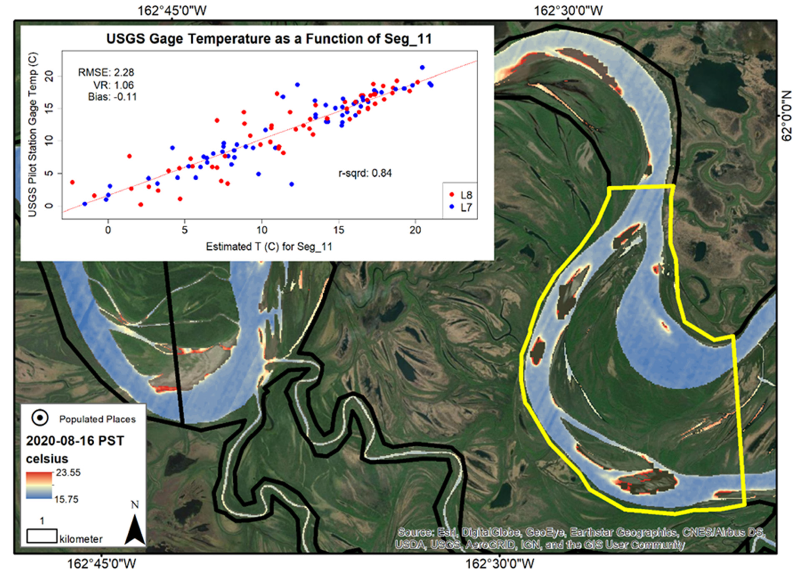
| 11 | 121 | 11.50 | 11.62 | 2.28 | 1.06 | −0.11 | 0.84 | 6.5 × 10−50 |
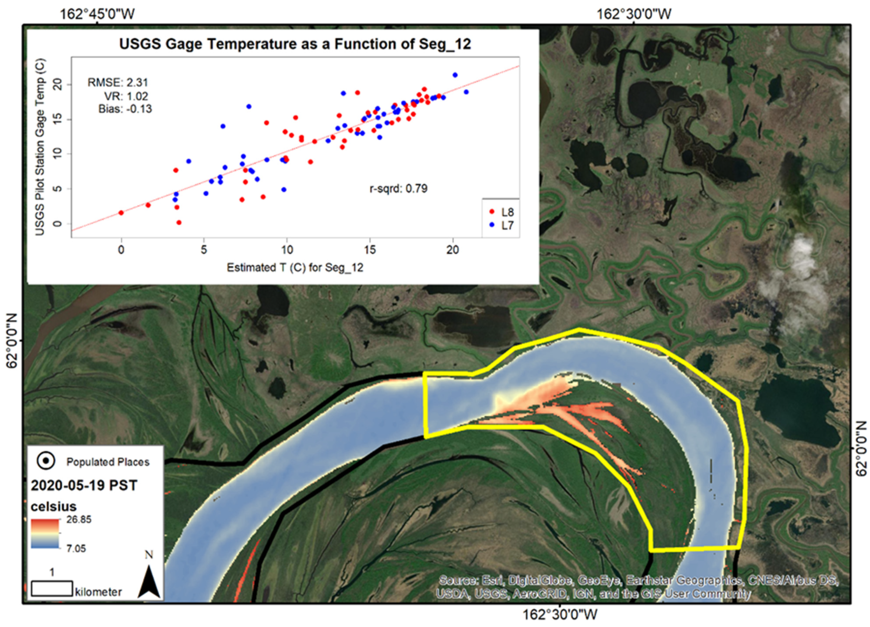
| 12 | 91 | 12.47 | 12.59 | 2.31 | 1.02 | −0.13 | 0.80 | 2.4 × 10⁻³² |
| 13 | 126 | 12.18 | 11.73 | 2.60 | 1.01 | 0.45 | 0.79 | 1.9 × 10−44 |
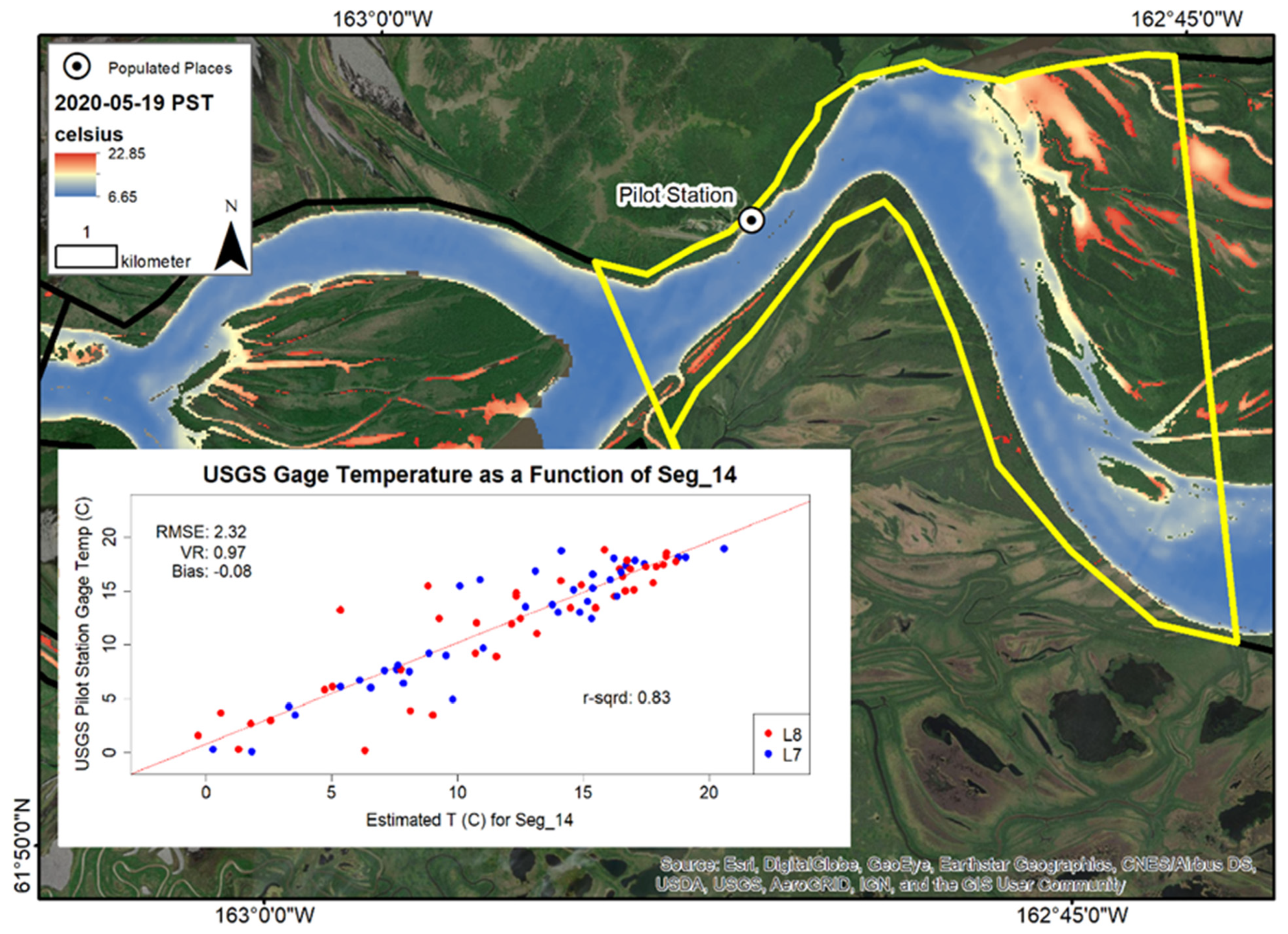
| 14 | 80 | 11.79 | 11.86 | 2.32 | 0.97 | −0.08 | 0.83 | 3.5 × 10⁻³² |
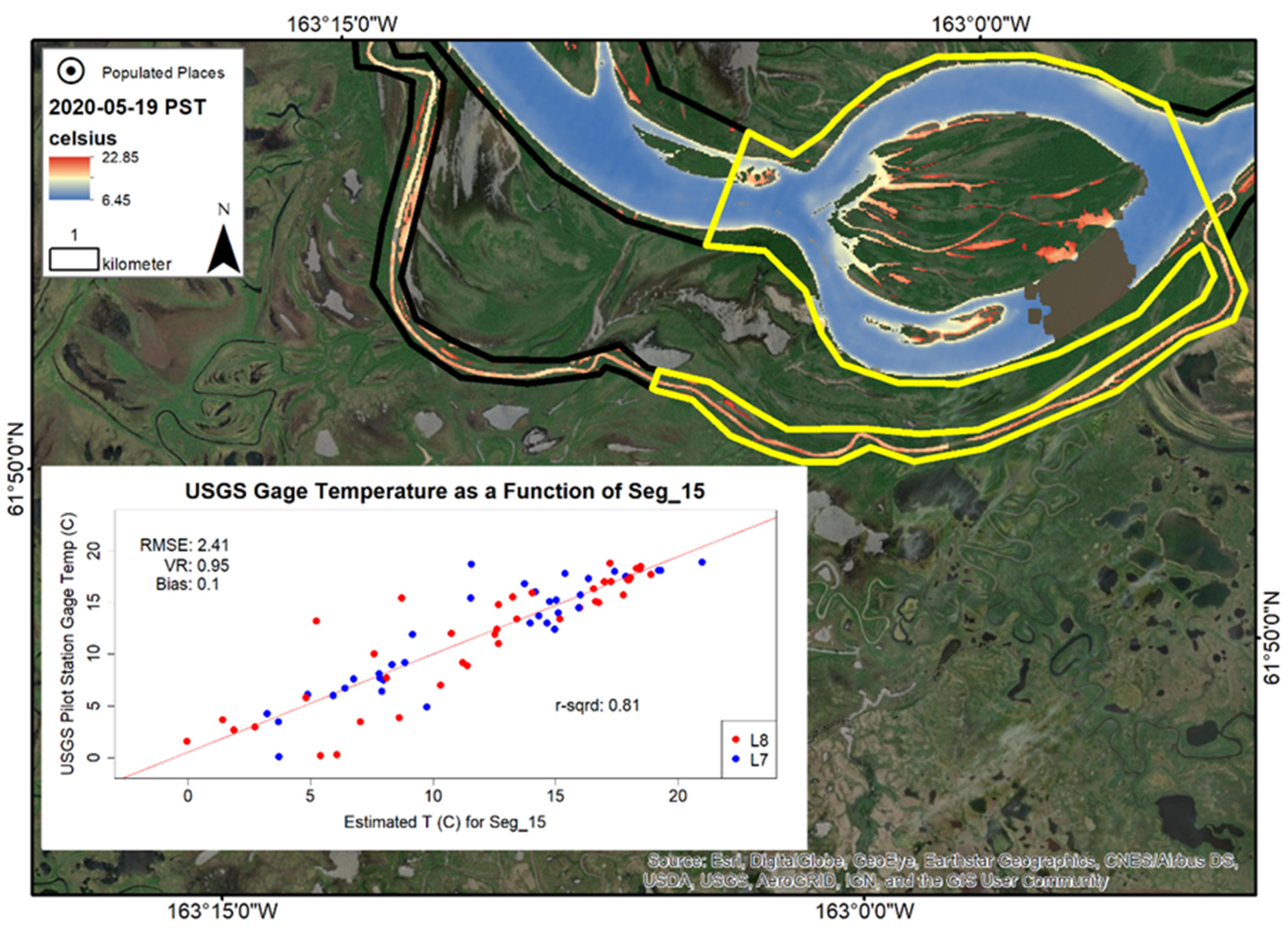
| 15 | 75 | 11.94 | 11.85 | 2.41 | 0.95 | 0.1 | 0.80 | 6.6 × 10⁻²⁸ |
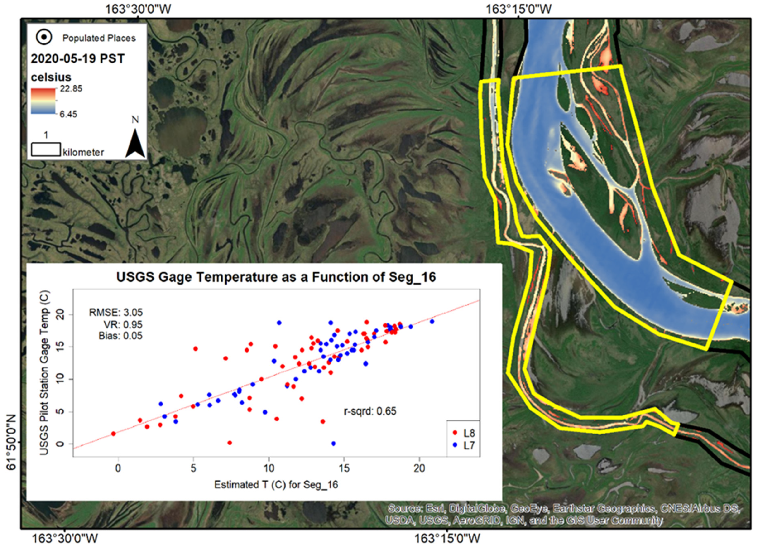
| 16 | 107 | 12.54 | 12.5 | 3.05 | 0.95 | 0.05 | 0.65 | 1.3 × 10⁻²⁵ |
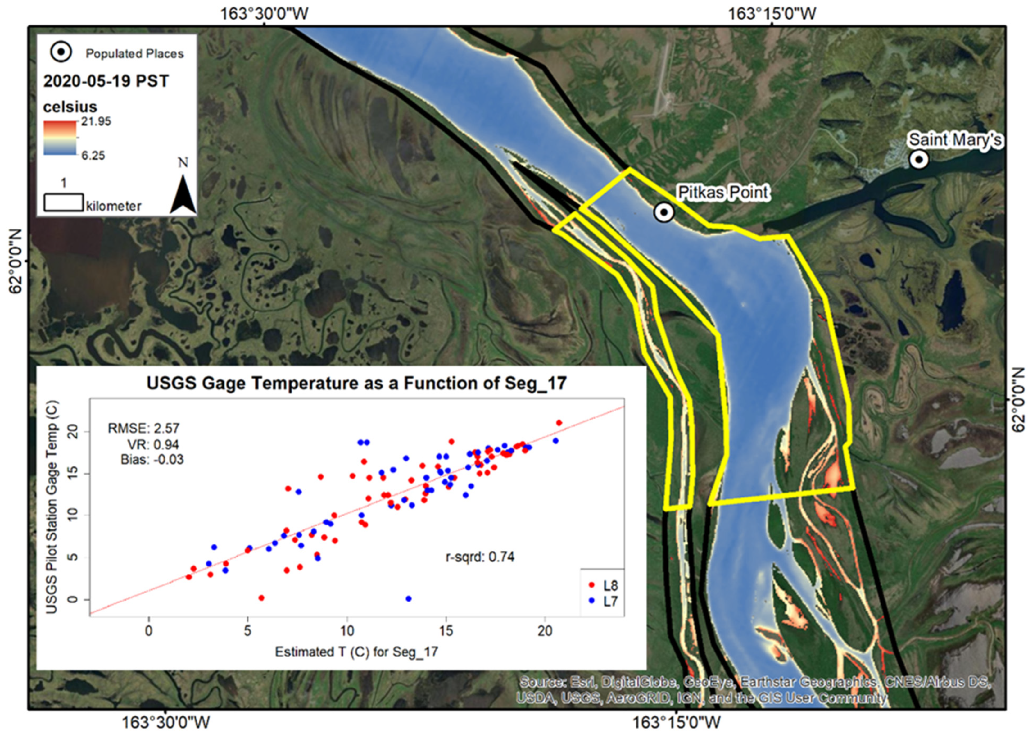
| 17 | 108 | 12.71 | 12.74 | 2.57 | 0.94 | −0.03 | 0.73 | 7.1 × 10⁻³³ |
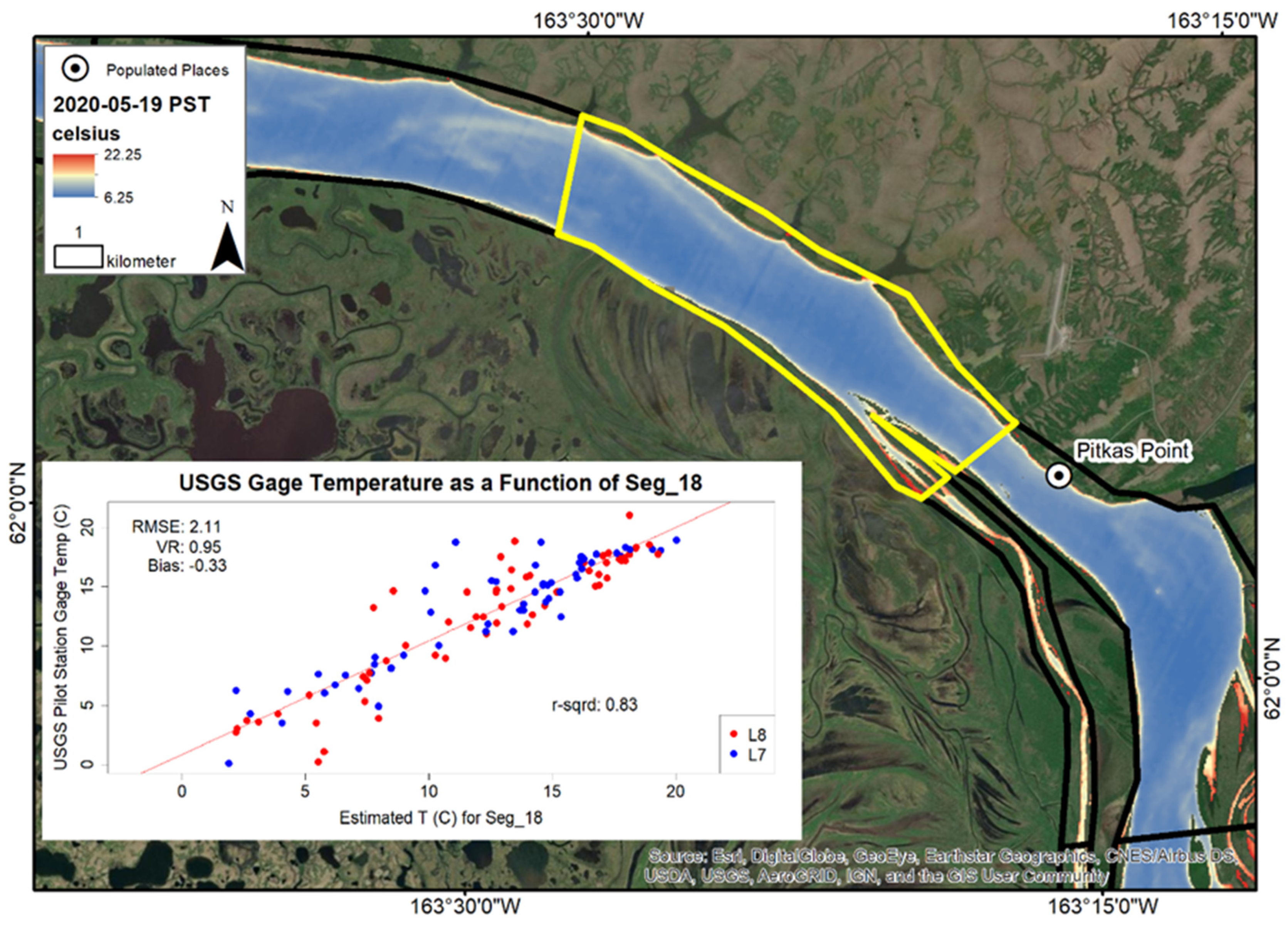
| 18 | 115 | 12.29 | 12.62 | 2.11 | 0.95 | −0.33 | 0.83 | 1.9 × 10−45 |
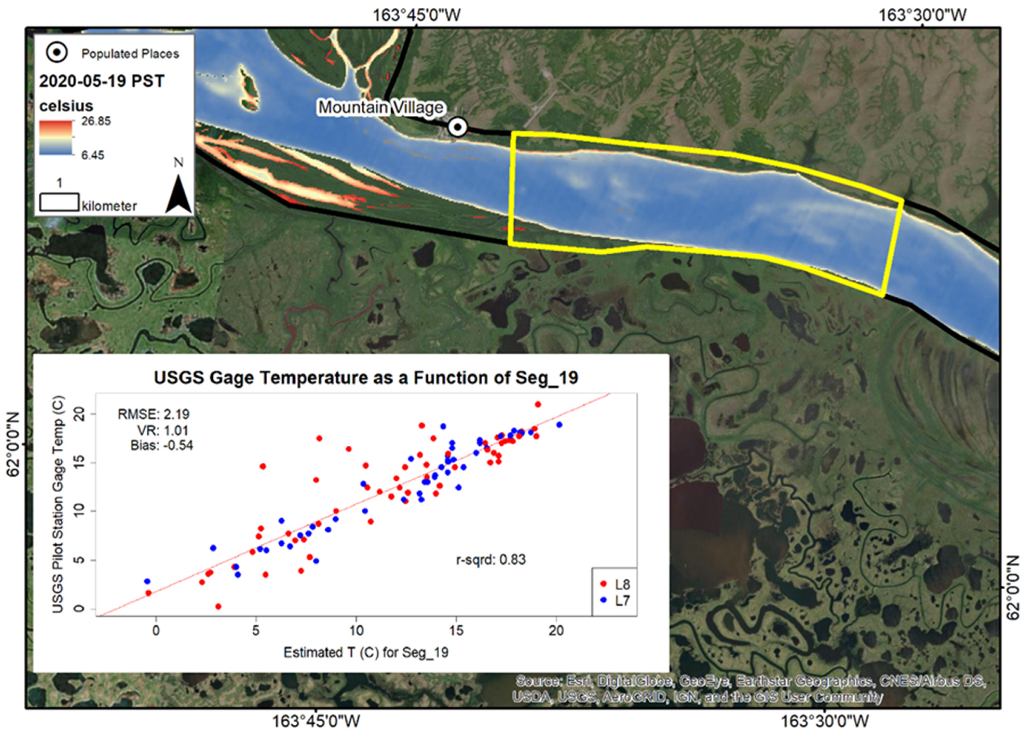
| 19 | 107 | 11.97 | 12.50 | 2.19 | 1.01 | −0.54 | 0.83 | 2.3 × 10−42 |
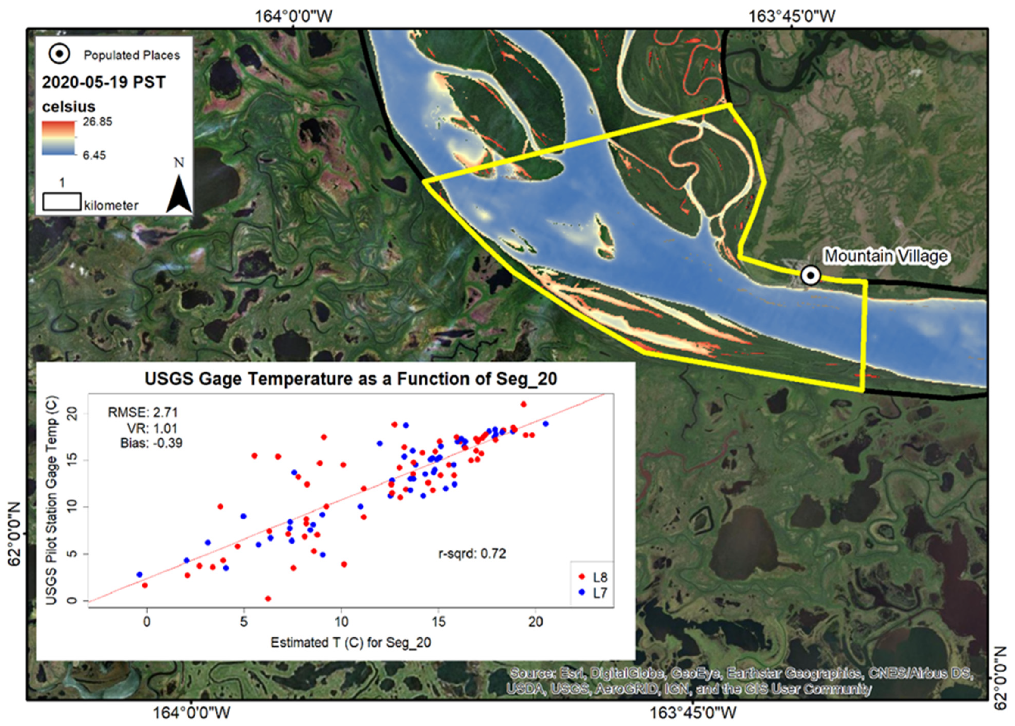
| 20 | 113 | 12.25 | 12.62 | 2.71 | 1.01 | −0.39 | 0.72 | 5.0 × 10⁻³³ |
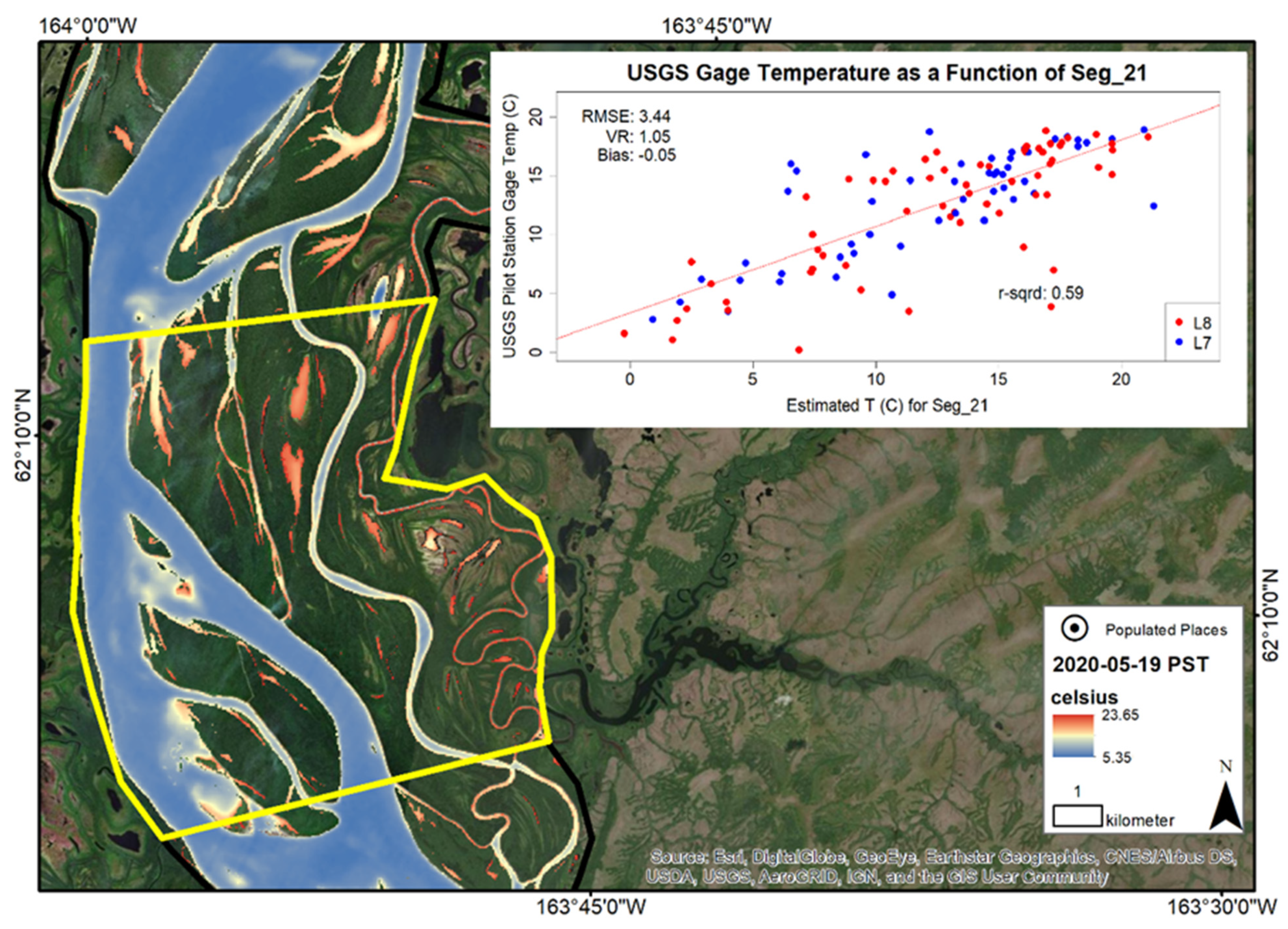
| 21 | 114 | 12.44 | 12.49 | 3.44 | 1.05 | −0.05 | 0.59 | 1.1 × 10⁻²³ |
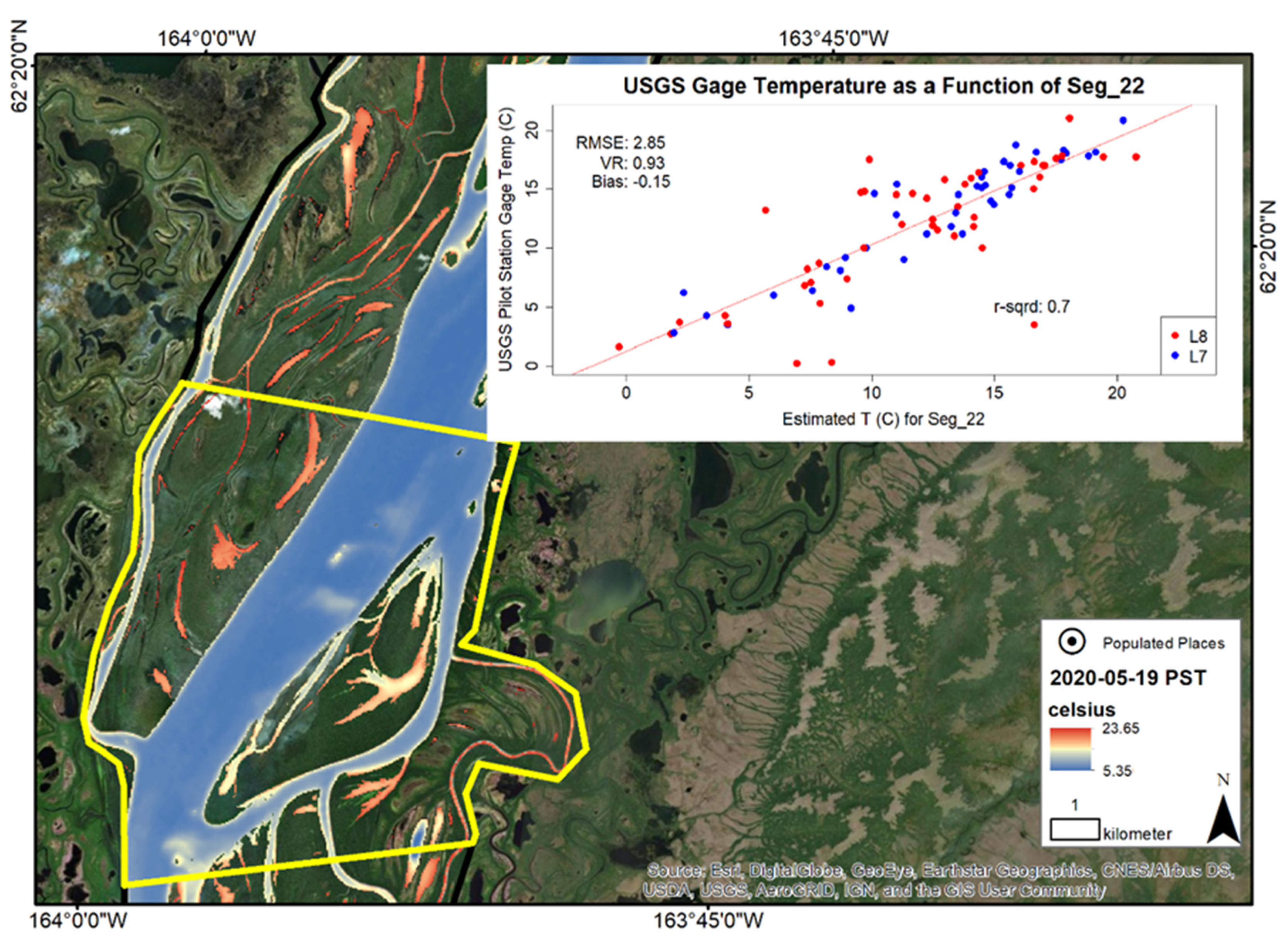
| 22 | 86 | 12.12 | 12.27 | 2.85 | 0.93 | −0.15 | 0.70 | 3.3 × 10⁻²⁴ |
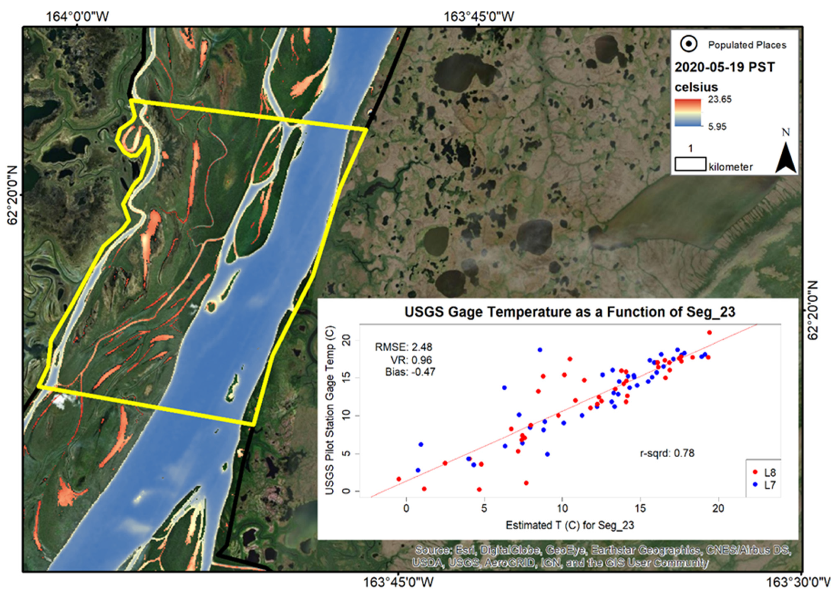
| 23 | 85 | 11.88 | 12.34 | 2.48 | 0.96 | −0.47 | 0.78 | 2.1 × 10⁻²⁹ |
| 24 | 87 | 12.38 | 12.54 | 2.26 | 0.97 | −0.17 | 0.80 | 1.5 × 10⁻³¹ |
| ARD Tile | 209 | 11.87 | 12.13 | 2.46 | 1.00 | −0.26 | 0.79 | 2.3 × 10−73 |
Publisher’s Note: MDPI stays neutral with regard to jurisdictional claims in published maps and institutional affiliations. |
© 2021 by the authors. Licensee MDPI, Basel, Switzerland. This article is an open access article distributed under the terms and conditions of the Creative Commons Attribution (CC BY) license (https://creativecommons.org/licenses/by/4.0/).
Share and Cite
Baughman, C.A.; Conaway, J.S. Comparison of Historical Water Temperature Measurements with Landsat Analysis Ready Data Provisional Surface Temperature Estimates for the Yukon River in Alaska. Remote Sens. 2021, 13, 2394. https://doi.org/10.3390/rs13122394
Baughman CA, Conaway JS. Comparison of Historical Water Temperature Measurements with Landsat Analysis Ready Data Provisional Surface Temperature Estimates for the Yukon River in Alaska. Remote Sensing. 2021; 13(12):2394. https://doi.org/10.3390/rs13122394
Chicago/Turabian StyleBaughman, Carson A., and Jeffrey S. Conaway. 2021. "Comparison of Historical Water Temperature Measurements with Landsat Analysis Ready Data Provisional Surface Temperature Estimates for the Yukon River in Alaska" Remote Sensing 13, no. 12: 2394. https://doi.org/10.3390/rs13122394
APA StyleBaughman, C. A., & Conaway, J. S. (2021). Comparison of Historical Water Temperature Measurements with Landsat Analysis Ready Data Provisional Surface Temperature Estimates for the Yukon River in Alaska. Remote Sensing, 13(12), 2394. https://doi.org/10.3390/rs13122394