Article

Near-Real-Time Flood Mapping Using Off-the-Shelf Models with SAR Imagery and Deep Learning

by
Vaibhav Katiyar
1,2,*,
Nopphawan Tamkuan
1,2 and
Masahiko Nagai
1,2
1
Graduate School of Sciences and Technology for Innovation, Yamaguchi University, 2-16-1, Tokiwadai, Ube, Yamaguchi 755-8611, Japan
2
Center for Research and Application of Satellite Remote Sensing, Yamaguchi University, 2-16-1, Tokiwadai, Ube, Yamaguchi 755-8611, Japan
*
Author to whom correspondence should be addressed.
Remote Sens. 2021, 13(12), 2334; https://doi.org/10.3390/rs13122334
Submission received: 31 March 2021 / Revised: 9 June 2021 / Accepted: 11 June 2021 / Published: 14 June 2021
(This article belongs to the Special Issue Remote Sensing Images Processing for Disasters Response)

Abstract

:
Timely detection of flooding is paramount for saving lives as well as evaluating levels of damage. Floods generally occur under specific weather conditions, such as excessive precipitation, which makes the presence of clouds very likely. For this reason, radar-based sensors are most suitable for near-real-time flood mapping. The public dataset Sen1Floods11 recently released by the Cloud to Street is one example of ongoing beneficial initiatives to employ deep learning for flood detection with synthetic aperture radar. The present study used this dataset to improve flood detection using well-known segmentation architectures, such as SegNet and UNet, as networks. In addition, this study provided a deeper understanding of which set of polarized band combination is more suitable for distinguishing permanent water, as well as flooded areas from the SAR image. The overall performance of the models with various kinds of labels and a combination of bands to detect all surface water areas were also assessed. Finally, the trained models were tested on a completely different location at Kerala, India, during the 2018 flood for verifying their performance in the real-world situation of a flood event outside of the given test set in the dataset. The results prove that trained models can be used as off-the-shelf models to achieve an intersection over union (IoU) as high as 0.88 in comparison with optical images. The omission and commission error were less than 6%. However, the most important result is that the processing time for the whole satellite image was less than 1 min. This will help significantly for providing analysis and near-real-time flood mapping services to first responder organizations during flooding disasters.

1. Introduction

The importance of surface water mapping can be understood by studying UN Sustainable Development Goals (SDGs), in which as many as four goals directly mention surface water monitoring, including food security (target 2.4), water-related ecosystem management (targets 6.5 and 6.6), and the effect on land (target 15.3). However, the most relevant target in this study is target 11.5 under goal 11 (sustainable cities and communities), which states “By 2030, significantly reduce the number of deaths and the number of people affected and substantially decrease the economic losses relative to the gross domestic product caused by disasters, including water-related disasters, with a focus on protecting the poor and people in vulnerable situations” [1]. In this context, near-real-time (NRT) flood mapping becomes very necessary.
Because flooding is a large-scale phenomenon and with the improved spatial, temporal, and radiometric resolution of satellite images, remote sensing becomes the obvious choice for flood mapping [2]. There are many works related to the extraction of surface water information, including floods, varying from different sensor types to different methods [3]. Huang et al., 2018 [3], mentioned that the number of related works with “surface water” or “flood inundation” and “remote sensing” has seen three- to seven-fold growth since the year 2000 in comparison to the previous decade. A similar trend was also observed in the case of the mapping surface water from SAR imagery [4]. Surface water and flood extent extraction studies using optical images have mainly focused on using water indices such as the modified normalized difference water index (MNDWI) [5], the automated water extraction index [6], and other rich spectral information [7]. Though many of these techniques [7,8,9] have provided good results, optical images carry an inherent limitation; namely, dependence on solar radiation. This limits the optical satellites image acquisition time only in the day, inability to penetrate cloud cover and get affected by the adverse weather conditions which are often prevalent during high-impact flood events [10]. Some studies have used multimodal information, such as combining optical images and LiDAR with synthetic aperture radar (SAR) images [11,12,13] and combining other ancillary information with SAR [14,15]. Although multi-modal-based models provide improved results due to the complementary capability, using a variety of data make it difficult to provide an NRT flood map because of more time in data acquisition and processing. Therefore, in this study, only SAR images were used. Flood mapping with only SAR images is generally categorized as two types: change detection using images captured before and during the flood, and water area detection using a single SAR image captured during the flood. Though change detection methods have the advantage of handling overprediction by providing additional information about water-like surfaces [16], an additional limitation that occurs with this method is finding an adequate reference image for flood detection [17]. When NRT imaging is required, it is necessary to have as few constraints as possible to speed up processing, which is why this study adopted flood mapping based on a single SAR image. For flood mapping from a single SAR image, the most well-known technique is thresholding with some algorithms, such as Otsu thresholding [18] and minimum error thresholding [19], with a global or tile-based approach [16]. Because global thresholding has a constraint of bimodality of data, which creates a problem in the case of full image processing, tile-based thresholding, and the split-based approach [20] have been proposed. However, with these methods, the choice of tiles plays an important role and the wrong tile may impact the threshold significantly [16].
Recently, the development of deep learning in the image processing field, especially deep convolutional neural networks (DCNNs), has enabled the development of new methods for automated extraction of flood extent from SAR images, as proposed in [21,22]. However, these studies used unpublished datasets, which makes it difficult to compare different models, and the use of commercial SAR images also makes it challenging to test methods on custom sites. This brings us to the real problem of NRT flood mapping with deep learning techniques: the absence of a SAR-based global flood dataset that provides enough diversity to generalize the model. The release of the Sen1Floods11 dataset [23] provided the opportunity for us to develop an off-the-shelf model that can be used for NRT flood mapping. However, to achieve better performance, the following four questions need to be answered: (1) What combination of band polarization is most suitable for flood mapping? (2) What is the effect of different kinds of labelling techniques (for training) on the performance of the models? (3) How do we make a model more flexible and scalable so that it can be applied to an actual flood situation and on the whole satellite image? (4) How do we apply the trained model to a different test site to validate the applicability of the off-the-shelf model?
Along with getting deeper insight into the four questions above, this study can help for the better development of future datasets related to flooding with SAR. In addition, the study has contributed to developing a whole pipeline for off-the-shelf model making. This similar strategy can potentially be re-used for other SAR satellites and further specialized flood mapping.
This paper is organized as follows. First, the details of the Sen1Floods11 dataset are discussed, along with the test site details and the data used for the test site. Then, the network architecture and training strategy are elaborated. After this, the testing steps, as well as validation data generation on the test site and the performance measures used in the study, are discussed. Finally, the results of the different models’ performance are discussed using detailed illustrations and explanation. The trained models, validation data used in this study, and results are uploaded at https://sandbox.zenodo.org/record/764863. The source code is available from the authors upon reasonable request.

2. Materials and Methods

2.1. Dataset Description and the Test Area

2.1.1. Sen1Floods11 Dataset
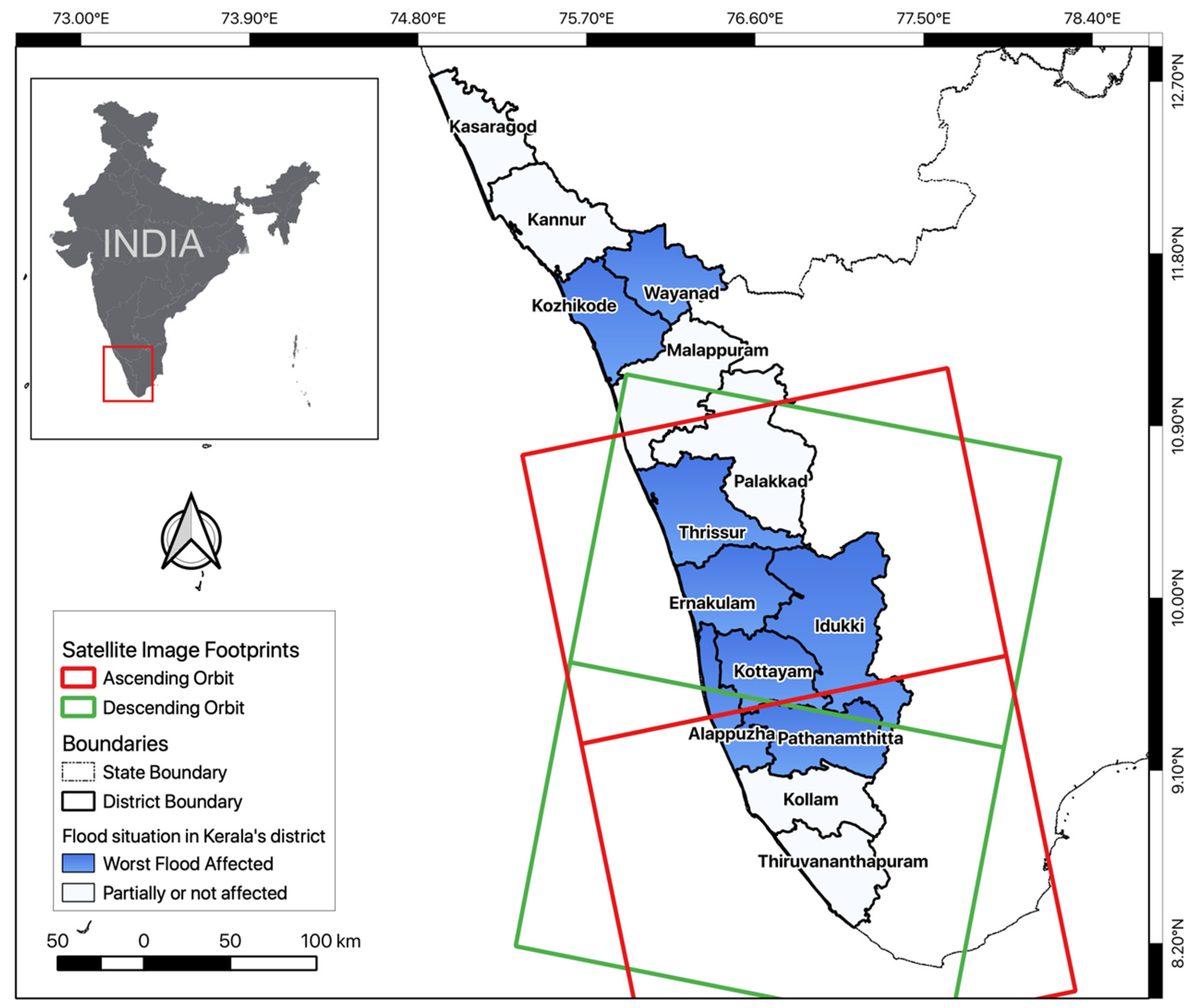
This study used the Sen1Floods11 dataset that was released during the 2020 Computer Vision and Pattern Recognition Workshop [23] and generated by Cloud to Street, a public benefit corporation. Details of the dataset are given below.
The dataset is divided into two parts, one containing data related to flood events and another for permanent bodies of surface water. The permanent water data include images from the Sentinel-1 satellite constellation and corresponding labels from the European Commission Joint Research Centre (JRC) global surface water dataset. We mainly used the flood events dataset in this study, which has two types of labels: weakly labeled and hand labeled. Weakly labeled here means that the labels have not been checked for quality, as they were generated through semi-automated algorithms that use certain thresholds to separate water and non-water areas. The weakly labeled data have two kinds of labels generated from Sentinel-1 and Sentinel-2 images, respectively. These labels are binarized images containing ones (for water pixels) and zeros (for non-water pixels). Sentinel-1 weak labels were prepared using the Otsu thresholding method over the focal mean-smoothed VH band. For creating the weak labels from Sentinel-2 images, expert-derived thresholds of 0.2 and 0.3 were applied over the normalized difference vegetation index (NDVI) and MNDWI bands, respectively. These weakly labeled data have not been quality controlled and over- or under-segmentation is possible. The hand-labeled data were created using information from overlapping tiles of both Sentinel-1 and Sentinel-2. The manual classification was performed using the Sentinel-1 VH band and two false-color images of Sentinel-2 (RGB: B12, B8, B4 and B8, B11, B4) that highlight the water areas in the optical images. The resultant labels are more accurate and have three values in the output: 1 (water pixels), 0 (non-water pixels), and −1 (clouds or cloud shadows).
Overall, 4830 non-overlapping chips were available to us that belong to flood events of 11 countries. Of these, 4385 chips are weakly labeled with corresponding S1Weak (Sentinel-1) and S2Weak (Sentinel-2) labels, while 446 chips are hand labeled and have corresponding quality-controlled labels. Each chip size is 512 × 512 pixels. All chips have overlapping Sentinel-1 and Sentinel-2 images. Sentinel-1 chips were created using dual-polarized Sentinel-1 ground range detected (GRD) images. As these images have been downloaded from the Google Earth Engine, each image was pre-processed using the Sentinel-1 Toolbox by the following steps: thermal noise removal, radiometric calibration, terrain correction using SRTM 30, and finally conversion of both bands’ values into decibels via log scaling. In contrast, Sentinel-2 chips are from raw Sentinel-2 MSI Level-1C images having all 13 bands (B1–B12). The 13 spectral bands represent the top of atmosphere reflectance, scaled by 10,000.
The hand-labeled data were split into three parts with a ratio of 60:20:20 into training, validation, and test sets. In contrast, all the weakly labeled data were used for training purposes only. In this way, the test set and validation set remained the same throughout, while training data could be changed according to our requirements, and we could do cross-comparison for different kinds of training data.

2.1.2. Test Area

The study area that was chosen for applying the off-the-self model is in the southern Indian state Kerala, as shown in Figure 1. In 2018, an especially devastating flood occurred in Kerala; this flood took more than 400 lives and affected millions more.
Figure 1 highlights the worst-affected districts in Kerala; western districts faced much more severe flooding than eastern districts because western districts are topographically flat (coastal plains). As mentioned in Table 1, four Sentinel-1 images of the affected area on the same date of 21 August 2018 were selected for testing. Two images were acquired during the ascending flight direction and two were acquired during the descending flight direction. The closest Sentinel-2 image of the same area is available for 22 August 2018. However, most of the area in this image has clouds. So finally, only the area belonging mainly to the Alappuzha district was selected because this image has no or very few pixels affected by clouds in the Sentinel-2 image. This was done to validate the detection from the Sentinel-1 image. In general, reference flood mask is generated using aerial images [20,24] or optical images such as Worldview [25], Sentinel-2 [26,27]. Therefore, authors adopted using Sentinel-2 image, which previously were successfully utilized for flood mapping [28], on their own and as a flood reference mask to validate the results [26,27]. To make a reference water mask from the Sentinel-2 image, MNDWI, false color composite using bands B12, B8, and B4 and the true-color composite using B4, B3, and B2 bands were used, along with this visual inspection was performed to maintain the accuracy of the mask.

2.2. Networks and Hyperparameters

DCNNs are composed of cascades of layers, executing mainly three important operations, convolution, downsampling and upsampling. The convolution layer uses a local kernel with a certain size, such as 3 × 3, over the image. This kernel traverses to the height and breadth of the input image and generates the convolved output [29]. The kernel elements can be understood as the weights which are learned in the neural network using backpropagation.
Max pooling layer, subsamples the input and give only maximum value as an output. This way the spatial dimension shrinks (downsampling) if the neighborhood size is chosen as 2 × 2 then the output value will be only the max of all the four values, producing the output quarter of its input size. Upsampling can be considered as reverse of the maxpool function as after upsampling the spatial dimension of the output increases.
Activation functions used in the DCNNs introduces non-linearity in the network which helps to map complex functions. One example of activation function is ReLU (rectified linear unit) is defined as f ( x ) = m a x ( 0 , x ) this means ReLU just let pass the positive values as it is while converting all the negative values to zero [30].

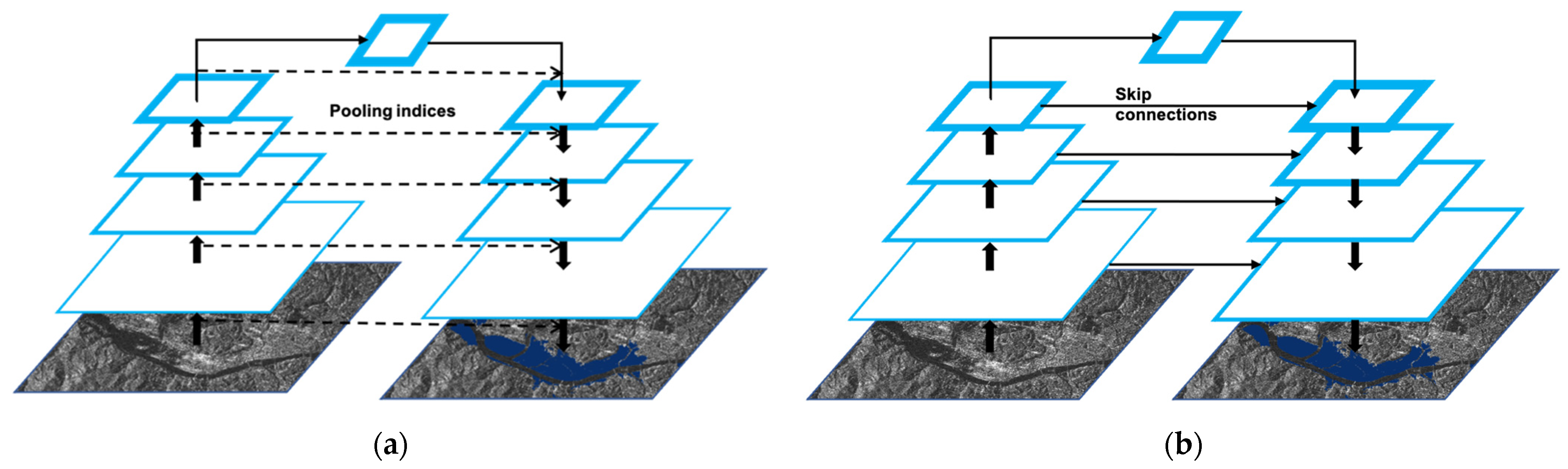
2.2.1. Networks Used

Variants of auto-encoders, namely, SegNet-like [31] and UNet-like [32] architectures, were selected for segmenting the water areas from Sentinel-1 chips. These networks, as shown in Figure 2, were selected because they are simple compared with other existing networks for segmentation such as HRNet [33], DANet [34], etc., and they also have shown great performance when the dataset is limited in size [32,35]. Both networks can be divided into two parts, the contraction phase (encoder path), and the expansion phase (decoder path). Each block in the encoder path contains two convolution layers that have a kernel size of 3 × 3 and the ‘same’ padding along with the batch normalization [30] and rectilinear unit (relu) activation layer. This is followed by a max-pooling layer with a size of 2 × 2 and a stride of 2. In this way, the convolution layer increases the number of features in the channel space (depth) while the max-pooling layer contracts the dimensions of the spatial feature space. Between both networks, the number of blocks in the encoder and decoder path remained the same, but the method for increasing the spatial size (upsampling) in the decoder section was the main difference. Here, UNet uses up-convolution along with the skip connections to use the features from previous layers, while in SegNet, up-sampling in the decoder section uses pooling indices that are computed in the max-pooling step of the corresponding encoder blocks. Thus, in the case of the SegNet, only spatial information is transferred from the lower-level layers, while in the UNet, the low-level feature space is also transferred to the high-level feature space and concatenated with it at the corresponding levels. This passing of the low-level features to high-level becomes possible due to skip connection which can bypass the intermediate layers [30]. The networks remain fixed across the training cases and in various band-combination inputs. This means only the shape of the input layer is modified while all intermediate and output layers remain constant.

2.2.2. Hyperparameters

For the entire study, the mini-batch size was selected as 16 and iterated over the whole dataset 200 times (epoch). The loss function used here was a custom loss function that used both Dice loss and binary cross-entropy (BCE) [29,36] in a weighted manner. While the Dice score mainly looks for the similarity of segmentation blob, BCE calculates pixel-wise variance. This means the dice score do capture the spatial information better than the BCE, which is why Dice loss was given a higher weight of 0.85, and BCE received a lower weight of 0.15. The Adam optimizer [37] was used for training optimization, with an initial learning rate of 0.01. The learning rate is decayed for faster convergence and to avoid over-fitting [29]. If there is no improvement (tolerance is set to 0.001) for continuously 10 epochs on a validation set, the learning rate reduced by the factor of 0.8. The minimum value for learning has been fixed to 0.0001. The training was performed on a single NVIDIA Titan-V GPU. The whole model development and training were performed using the Tensorflow platform along with the Keras library in Python.

2.3. Training Strategy

In total, three training cases were selected: (1) training using Sentinel-1 weak labels, (2) training using Sentinel-2 weak labels, and (3) training using more accurate hand labels. In each case, four SegNet-like and UNet-like networks were trained for the different band combinations: using both polarizations (VV, VH), using only cross-polarization (VH), using only co-polarization (VV), and using a ratio as the third band, making the input as VV, VH, and VH/VV. Here it should be noted that the VV and VH bands are already log scale, so the values of each pixel ranged between −50 and 1 dB. These inputs were normalized using min-max values so that the resultant values were between 0 and 1 before they were passed on for training. Additionally, for the calculation of the VH/VV ratio, we simply subtracted the log-scaled VH and VV bands due to the log properties:
log ( VH VV ) = log ( VH ) log ( VV ) .
Later, transfer learning was also used to explore the option of making our model more adaptable and scalable. For this step, three cases were selected. In the first case, the whole network was retrained and pre-trained weights were used as starting weights rather than random weights, which are typically used during training from scratch. In the other two cases, we conducted training only during the contraction phase (encoders) while freezing the expansion phase (decoders) and vice versa. Transfer learning has various benefits, such as the ability to include more training data in the future to further tune the network, faster convergence due to pre-trained weights [38], and the possibility of extending the trained model to be used with a new set of satellite images, such as from a different SAR satellite [39].

2.4. Testing

2.4.1. Testing on the Test Dataset

Three test cases were selected: all surface water detection, only permanent water detection (using corresponding JRC labels), and flooded water detection (difference between all water and permanent water). Because some of the image chips did not have any permanent water, they were removed from the test set of permanent water. In total, we had 90 test image chips for all water and flood water detection, and 54 chips for permanent water detection. All the trained networks, totaling 24 networks (SegNet and UNet), were tested over the given three test cases.

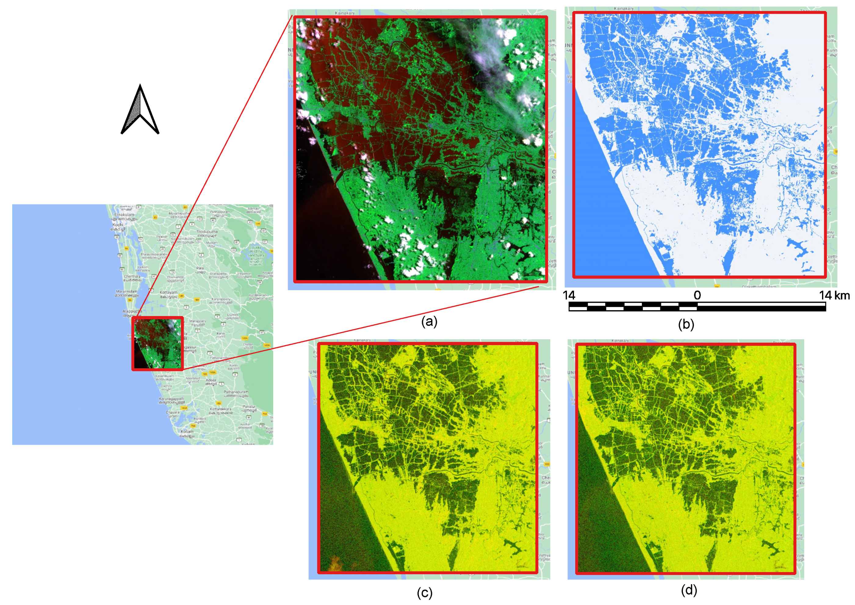
2.4.2. Testing as an off-the-Shelf Model on the Whole Image during the 2018 Kerala Floods

To verify the generalizability of the trained model for use as an off-the-shelf model during an emergency, a completely different flood event, the 2018 Kerala floods was selected. The first validation flood mask was prepared using the Sentinel-2 image. Although most of the Sentinel-2 image was covered by clouds, fortunately, the area most affected by the flooding had minimal cloud cover, so that area was selected, amounting to 794 km2 (Figure 3). After obtaining the desired area, the semi-automatic classification in QGIS was used over the Sentinel-2 bands B2, B3, B4, B8, B11, and B12 along with the MNDWI. In this step, certain regions of interests for water pixels were manually chosen across the selected area, after which classification was performed. However, this classification still had numerous errors and cloud obstructions. Thus, after the classification was complete, manual inspection was performed to further improve the classified results. In the end, these accurate classified results were exported as a binary flood mask, and this mask performed the role of ground truth in the validation phase.
The Sentinel-1 images were first pre-processed using the European Space Agency’s snappy package in Python to sequentially perform thermal noise removal, radiometric calibration, speckle filtering, and terrain correction. As the selected area lies where two satellites images from the same flight direction meet, so both images were merged and gap-filled using QGIS. The same method was applied to the two images from other flight direction as well. After this, two separate methods were employed for water area classification. The first is a thresholding method where a threshold was selected based on a combination of minimum distance and the Otsu method, which was implemented using scikit-image learning libraries. For another method, our best-performing trained model (after transfer learning), generated in the previous step, was used on the pre-processed image to obtain a flood map as binarized output. The whole image with a size of 13,797 × 7352 pixels was processed within 1 min and transformed into a binarized output. After this, the same area as that selected for the Sentinel-2 was clipped from the output for evaluation purposes.

2.5. Accuracy Evaluation

Four indicators were adopted to measure the performance of the proposed approach over the ground truth, as well as for the comparison with the thresholding method: Equation (1)—intersection over union (IoU), Equation (2)—F1 score, Equation (3)—omission error, and Equation (4)—commission error. These are defined as:
IoU = Ground   Truth Predicted Ground   Truth Predicted ,
F 1   Score = 2 Precision Recall Precision + Recall = T P T P + 1 2 ( F P + F N ) ,
Omission   error = F N F N + T P ,
Commission   error = F P F P + T P ,
where TP, FP, and FN denote the true positive, false positive, and false negative pixels, respectively.

3. Results

3.1. Results on the Test Dataset

Figure 4 and Figure 5 show the different models’ mean IoU (mIoU) over the whole test set for SegNet and UNet, respectively. The x-axis shows the training cases, while the y-axis represents the mIoU. The detailed quantitative results from each network along with the respective errors are presented in Table 2 and Table 3. Columns in the table represent the three detection test cases, namely, permanent water, flooded water, and all surface water. For each test case, the three evaluation criteria, mIoU, omission error (Om.), and commission error (Comm.), as used in [23], are presented. In the rows of the tables, the three training cases, namely, training using Sentinel-1 weakly labeled, Sentinel-2 weakly labeled, and hand-labeled data and their corresponding results are given. Each training case further has four variations consisting of different combinations of SAR bands. Along with our results, the baseline results from [23] are also shown for each training case, as well as Otsu thresholding results for better comparison.
In both types of networks, a common pattern can be seen. For the permanent water, the band combination of VV, VH and VH/VV ratio performed best in most of the cases, while in cases of flooded water and all surface water, the input with both polarizations VV and VH gave the best results. Note that when we used only the co-polarized band (VV), the network trained on weak labels performed worst, especially in the case of flooded water detection and all surface water detection, with a very high omission error. The cause can be understood by the property of SAR backscattering, which in the case of flooded vegetation or agriculture field may show very high backscattering in the co-polarized band due to double bounce (caused by the small wavelength of C-band SAR) [40]. A more detailed explanation is provided in Section 4.
In contrast with the results in Bonafilia et al. [23], where the best results came from Otsu thresholding for permanent water, our results clearly show that both SegNet and UNet convincingly surpass the benchmark data by Otsu thresholding, as well as the baseline results, in all training cases. However, other results for the flooded water and all-surface water are in sync with [23], as the best detection in the case of SegNet, as well as UNet, comes from the models trained using Sentinel-2 weak labeled dataset. Moreover, in the case of flooded water, our models show as much as 50% enhancement over the baseline and for all surface water also our model shows an improvement of around 40% with the UNet model trained with the hand labeling dataset.
Overall, the UNet-like networks outperformed the SegNet-like networks in detecting the flooded water and all surface water, which is the target in the study. One of the reasons may be the use of skip connections, which propagate the shallow layer features to the deeper layers, helping to create a better feature set for pixel-level classification. For this reason, subsequent processing was done using UNet only. This means that features from the encoder layers played a more important role in processing the SAR images, and this was further proved when transfer learning was used. In other words, encoder retraining gives better results than does decoder retraining.
Weak labelling technique has the advantage of creating a larger set of training samples in an automated way in a shorter time and less manpower than the hand labeling. A larger number of training samples helps in finding greater insight. However, hand-labeled data have consistency and include cases that could not be captured by weak labelling techniques. Therefore, transfer learning was employed to take advantage of both situations, namely, more samples for generalization and accurate labels for tuning. As our focus in the study is flood mapping, the model that was trained using Sentinel-2 weak labels with both polarization bands (VV and VH) was selected for transfer learning because it performed best among all other band combination, for “flooded water” and “all surface water” detection. Then, transfer learning was employed on it using hand-labeled data and retraining it for the three cases, namely, retraining the whole model, retraining only the expansion phase, and retraining only the contraction phase, with the pre-trained weights. The results are presented in Table 4. Overall, the model retrained on the encoder part showed the best result and that was used for real-time flood area detection at the chosen test site.
To estimate the overall performance of the model for all test cases when models are trained using a hand-labeled dataset, a k-fold cross-validation procedure was carried out. The result of which is included in Appendix A.

3.2. Results on Test Site

The model resulting from the transfer learning performed notably well, and it was used on the test site in both ascending and descending flight directions. As shown in Table 5, it gave a better result than did the thresholding method. Moreover, the omission error was reduced significantly from around 16% to 6%, which is a very important criterion in emergency mapping, where omission error should be as low as possible. This means that false negatives should be fewer, even when some false positives may creep in. False negatives are a problem because leaving a flood-affected area off the map may lead to bad decision making—such as failing to evacuate or people travelling into the flooded regions.
Figure 6 shows the merged SAR images of the ascending flight direction and corresponding combined result of the surface water detection by Deep learning (our method) and Otsu thresholding. In the detection result, the white and black pixels are representing that both methods have classified the same either water or non-water, respectively. Contrarily to the red and cyan pixels which illustrate that both methods have classified differently. Cyan pixels imply that our method has classified the pixels as water whereas the thresholding method classified it as non-water and just the opposite in the case of Red pixels. In general, thresholding suffers from the noise in the output, as is visible in the combined results in terms of salt and pepper noise, as well as in the yellow and green insets. Owing to such kind of noise, a post-processing step, such as morphological erosion-dilation or minimal mapping unit application [16], is required after thresholding. The yellow rectangle displays a partially flooded agricultural area that was detected successfully by the deep learning model (in cyan color). In addition, the area shown by the green rectangle, which contains a few oxbow lakes on its far-right side, was successfully segmented by our model. In contrast, the blue rectangle shows the area around Kochi Port, which is one of the largest ports in India and docks multiple large vessels. This area produced some of the brightest pixels, and our method was not able to detect water in that area, while the thresholding method was able to achieve better results (red pixels). One of the reasons that the water was not detected by our method is that deep learning models learn the contextual information through spatial feature mapping, and it is a rare phenomenon to have water pixels covered by brighter pixels (in this case from ships). One way to detect such kind of rare events is by including few of the similar pattern in the training set or using some other ancillary data.

4. Discussion

The results presented in Section 3 allow us to make the following observations:
(1)
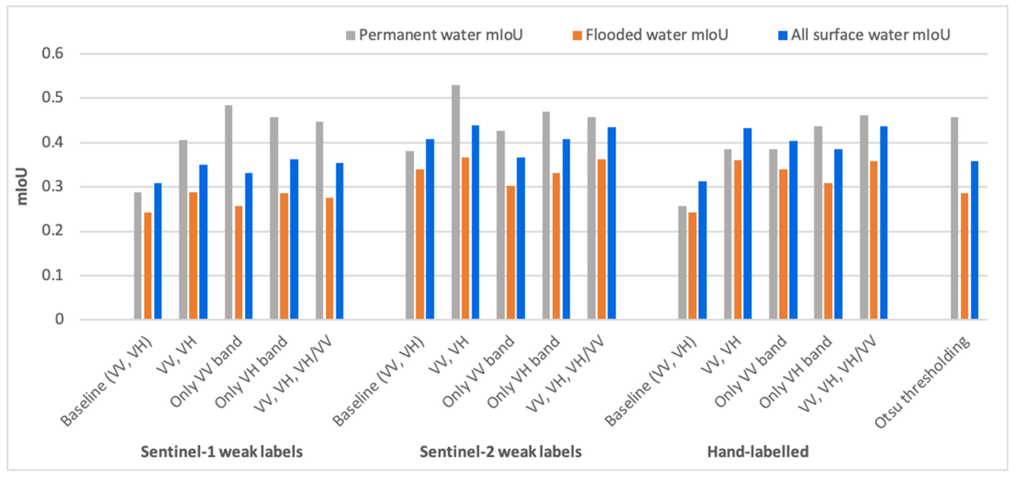
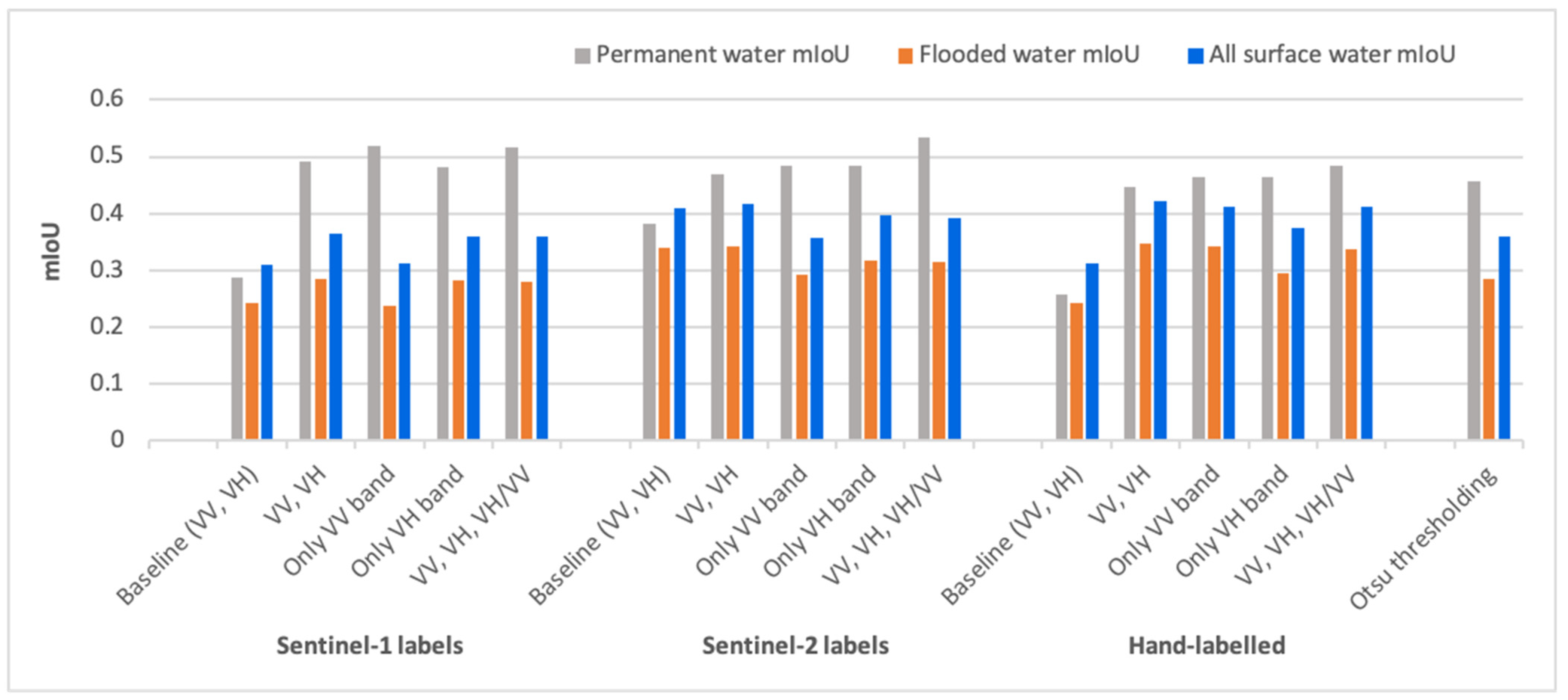
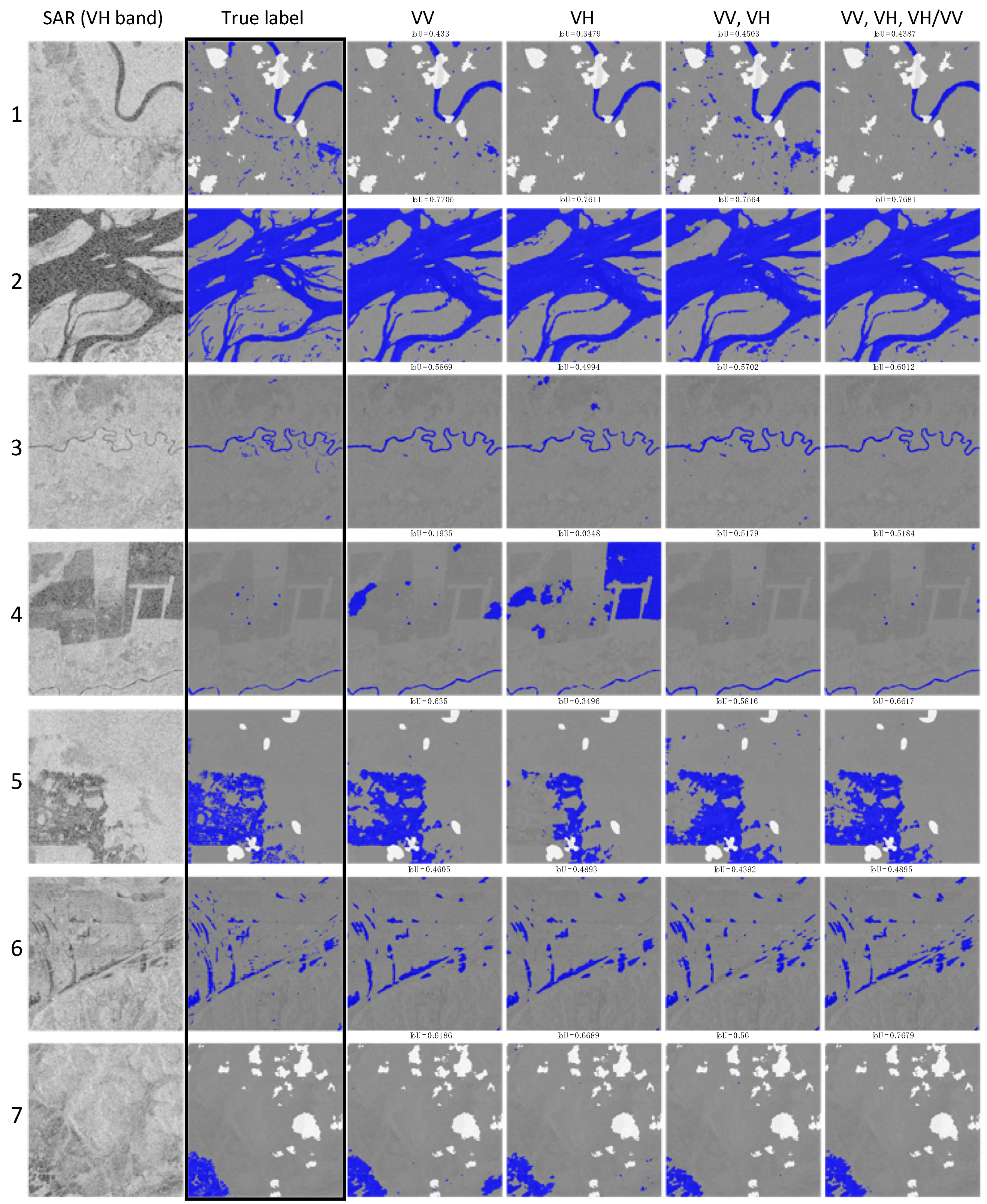
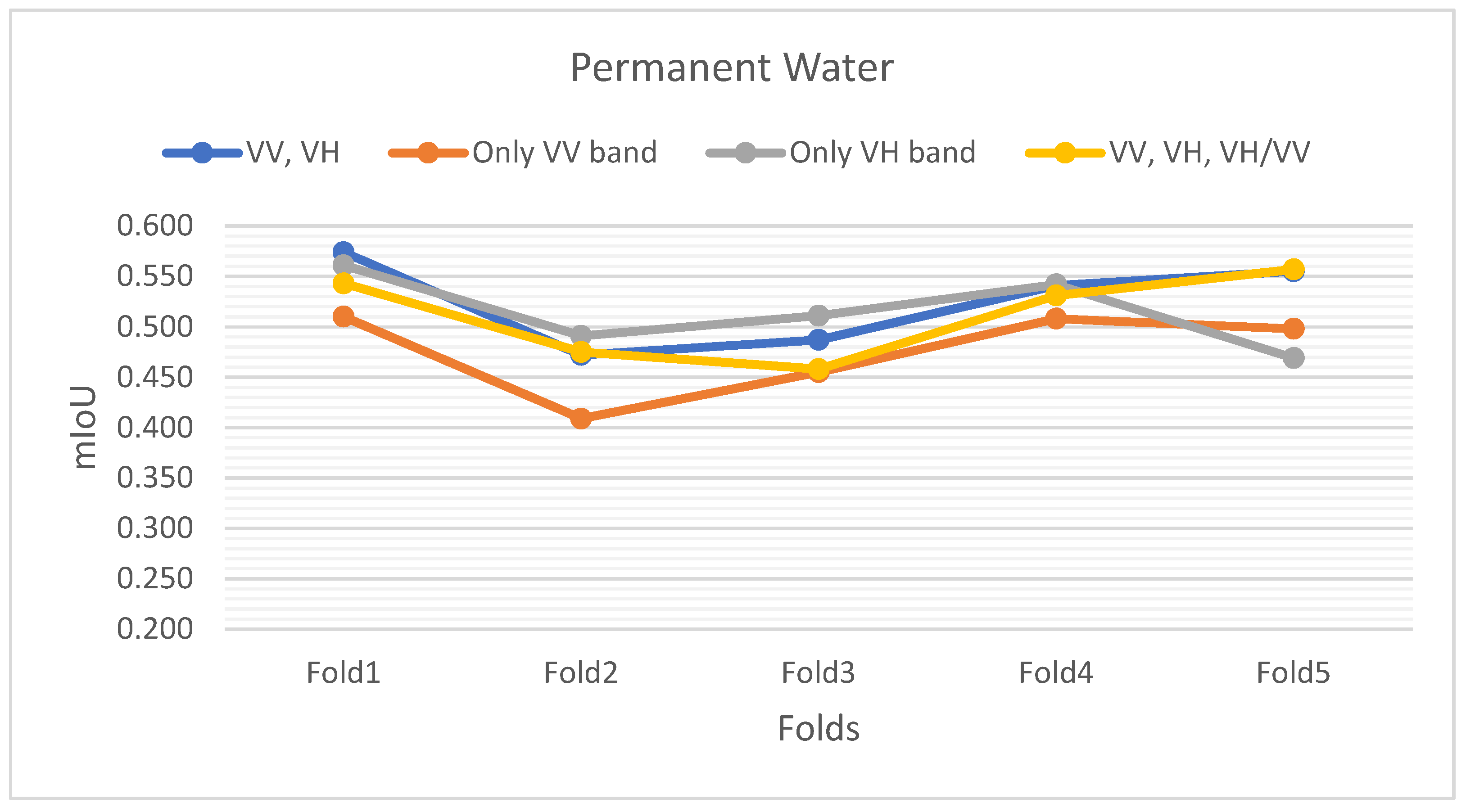
When the labels are weak, models trained on the co-polarization VV band performed poorly in comparison to models trained on the cross-polarization VH band. One of the reasons can be the high sensitivity of co-polarization towards rough water surfaces, for example, due to wind, as described by Manjushree et al. [41] and Clement et al. [26]. However, for hand-labeled data, VV performs better than VH, especially for flooded areas. Figure 7 shows the results from the models trained on different band combinations. Because the training set here was hand-labeled, VV performed mostly better than VH bands except in the rows 6 and 7. One of the interesting outcomes was that the three bands combined (VV, VH, and their ratio) gave the best results, except for the first row in Figure 7. This combination provided very good improvement in some of the difficult test cases, as in rows 5–7. This was particularly interesting as no new information is provided in the third band, it is just the ratio of already present input bands.
(2)
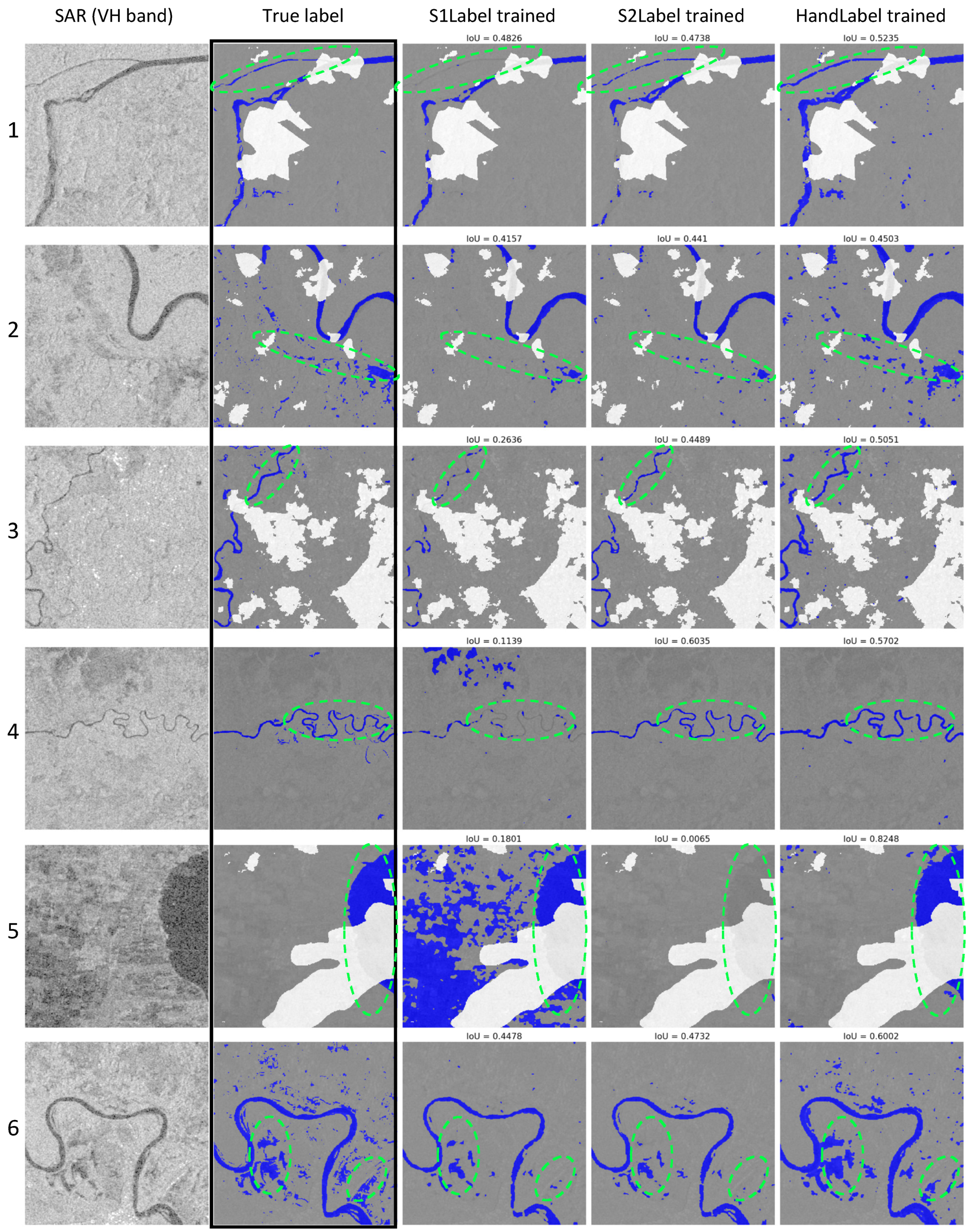
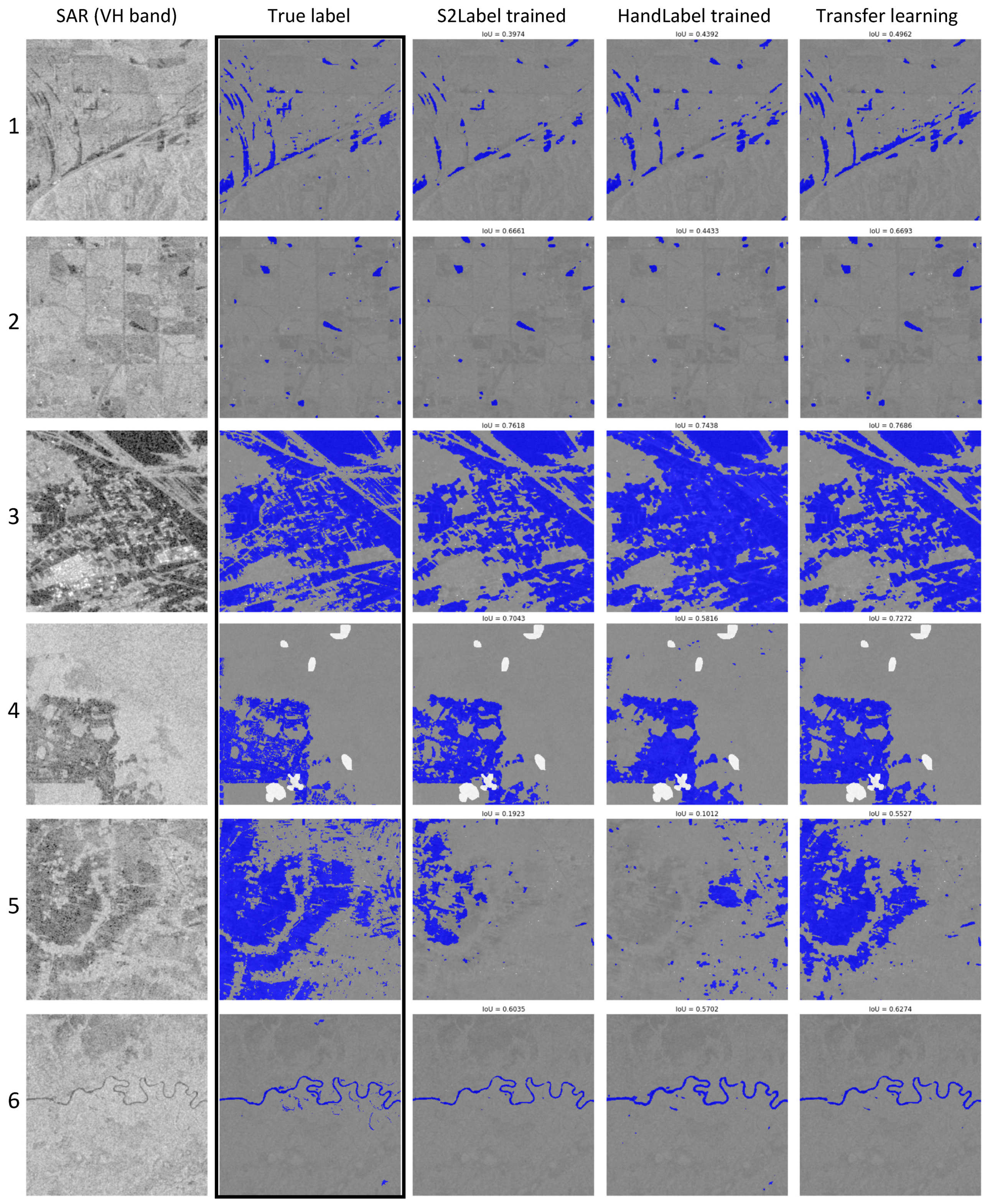
Models trained on Sentinel-2 weakly labeled data gave better results in comparison to Sentinel-1 weakly labeled data, which is consistent with the results of Bonafilia et al. [23]. Moreover, the models trained on hand-labeled data approximately matches the accuracy of the models trained with Sentinel-2 data and sometimes even beat them despite limited samples, which goes against the results of Bonafilia et al. [23], who concluded that hand-labeled data are not necessary for training fully convolutional neural networks to detect flooding. We have demonstrated that models trained with hand-labeled data perform better throughout, as shown in Table 2 and Table 3. Figure 8 shows a few examples of the improvement achieved by hand-labeled data. However, sometimes models trained with hand-labeled data give over-detection, as can be seen in the red circled areas in the first and last rows of the figure.
(3)
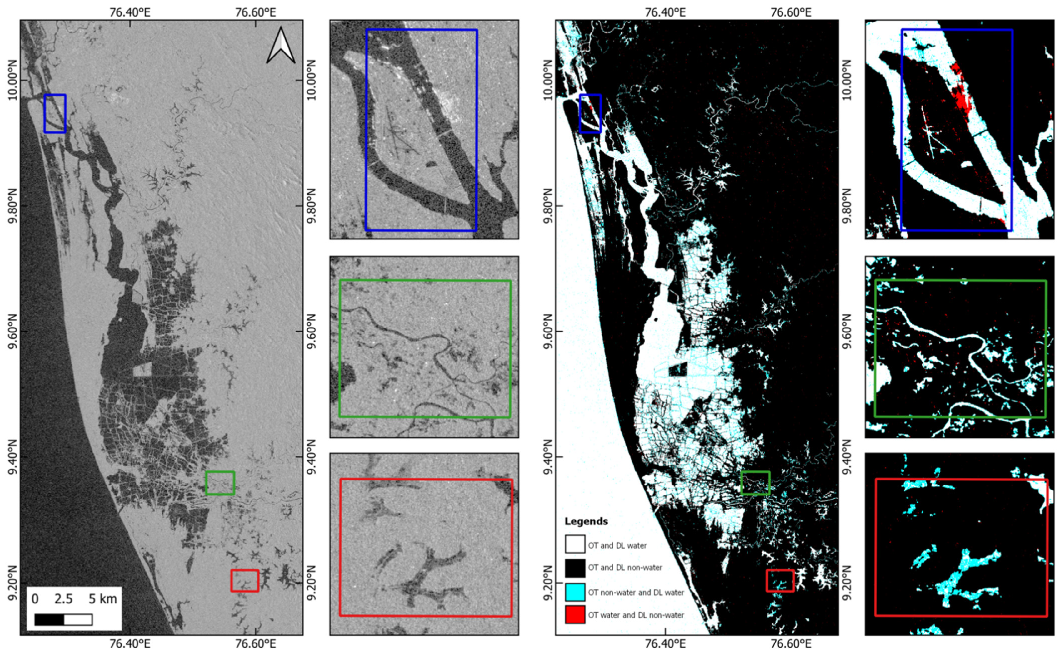
Successful implementation of transfer learning proves two things: first, there is no substitute for more accurate labels (hand-labeled data) as can be seen by the improved results. Second, that it is a good approach to generate many training samples automatically and a model trained on it gives better generalization. This is because more samples help in covering diverse cases and varieties of landcover. Further, we can use transfer learning to tune the model for our given test set. However, another interesting result is that, for finding surface water in SAR images, general features play a larger role than do specific features. As explained by Yosinski et al. [42], layers close to the input, encoder blocks in our case, are responsible for general feature extraction, and deep layers are responsible for obtaining specific features. In our experiments, freezing the expansion phase and retraining the contraction phase gave the most favorable result. This can be further explored with different architectures; if the same behavior persists, then we may use many shallow layer networks, making an ensemble to detect water areas from SAR images without wasting too many resources. The enhancement in water area detection using transfer learning is presented in Figure 9. Some of the examples, such as rows 1, 2, and 5, show significant improvement.
(4)
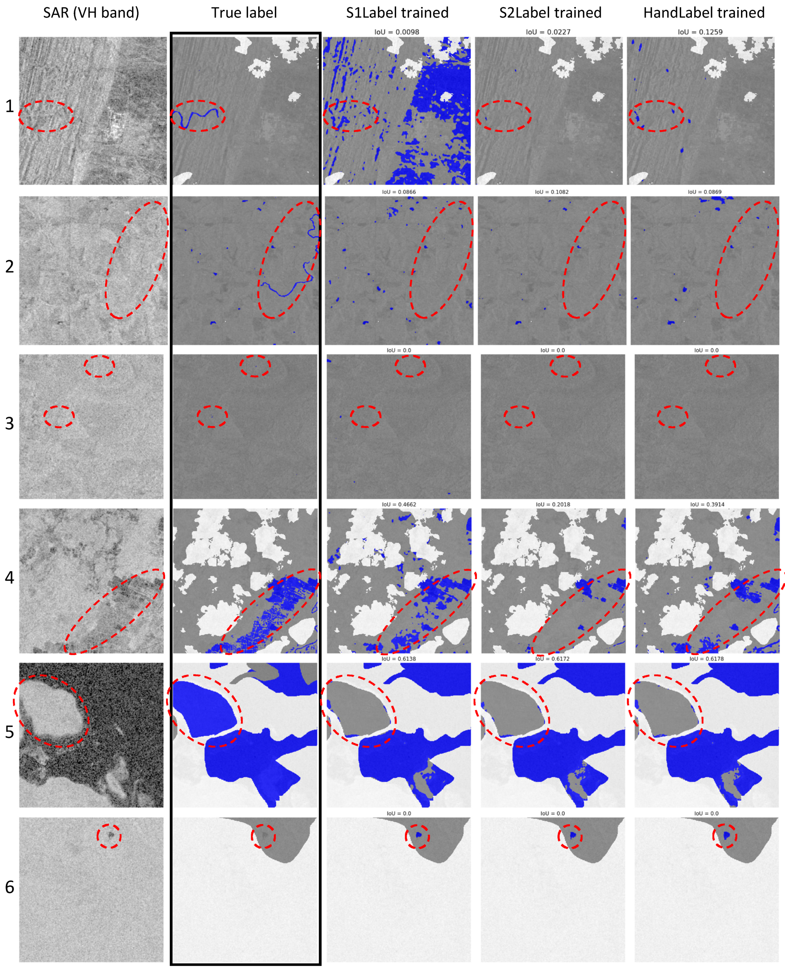
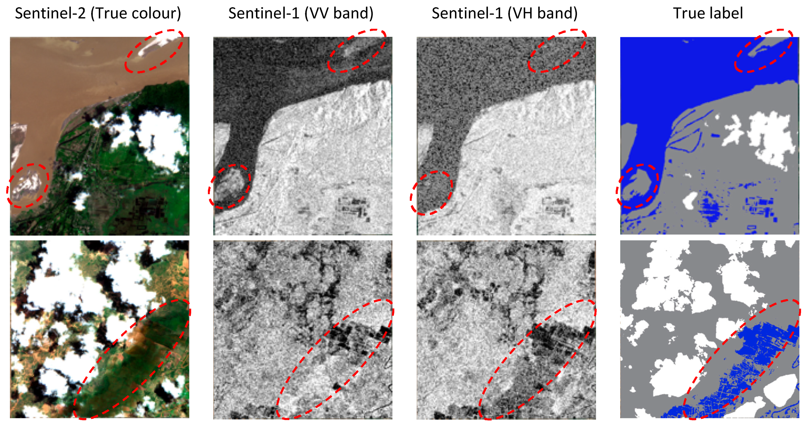
If we look only at mIoU in the test dataset, then its value, which was less than 0.5, does not present a good picture of the surface water detection. However, if we see some examples of the test set true labels along with the detected mask, such as in Figure 8, where we can see that the detection is quite accurate, especially by the model trained on hand-labeled data. Similar accuracy is seen in Figure 9, which shows the results of transfer learning models. Some of the reasons for low mIoU can be understood in Figure 10. In rows 1 and 2 of Figure 10, where a very narrow stream has been labeled, this stream is either not visible in SAR image due to mountainous terrain (row 1) or trees growing along with it (row 2), and it becomes difficult to identify any significant water pixels in the SAR image. Here we also need to take care of the SAR imagery geometric effects due to the side looking imaging principle, this may miss the water bodies such as river or small lakes behind the shadow or under the layover effect in the mountainous region [43]. Another issue is having very small water bodies containing very few pixels scattered over the whole image (row 3). We need to consider that spatial resolution of Sentinel-1 IW-GRD images is 5 m × 22 m in range and azimuth respectively, so smaller water bodies cannot be detected [43]. In this case, even though very few numbers of pixels were miss detected but the IoU will be near zero, affecting the mIoU of the whole test dataset. A few incorrect labels are present in the test dataset. Some examples of this are shown in rows 5 and 6, where the red ellipses show the locations of incorrect labels. In these situations, even though our model is performing quite well, the IoU becomes very low or in some case goes to zero, such as in the last row. Whereas, according to the given label, there are no water bodies, so the intersection will be zero and the union will be the detected water body pixels, which will result in an IoU of zero. Moreover, there are also many possible scenarios where, due to the special properties of the SAR, the detection is not accurate, such as in the case of row 4 in Figure 10. This area was flooded in a field with sparse vegetation, as can be seen in the true-color image in the last row of Figure 11. This creates a double bounce from the specular surface of the water and vegetation in the co-polarized band (VV). This anomaly is the reason that the model is not able to identify it as a flooded field. A similar example is shown in the first row of Figure 11, where sand deposits in the river have high backscatter in the VV band. One possible reason for the high backscatter is the presence of moisture in the sand which increase the dielectric constant, so the reflectivity. In addition, the VV band is in general more susceptible to surface roughness, so higher reflectivity along with roughness may be the reason for high backscatter [40]. These special cases can be detected by the model if there are enough training samples that also have similar properties.
Figure 7. Results from the models trained using different band combinations with the hand-labeled dataset. The colors in true labels (hand labeled) and other results represent water (blue), non-water (gray), and white (clouds).
Remotesensing 13 02334 g007
Figure 8. Results of the models trained with bands VV and VH combined over all three training sets. Areas inside the green ellipses show significant changes. The colors in true labels (hand labeled) and other results represent water (blue), non-water (gray), and white (clouds).
Remotesensing 13 02334 g008
Figure 9. The improved result, achieved by using transfer learning. Results are from the model trained using the VV and VH bands combined and the Sentinel-2 weakly labeled dataset and retrained using the hand-labeled dataset. The colors in true labels (hand labeled) and other results represent water (blue), non-water (gray), and white (clouds).
Remotesensing 13 02334 g009
Figure 10. Major errors (circled by red dotted lines) in results obtained from the model trained using the VV and VH bands with the hand-labeled dataset. The colors in true labels (hand labeled) and other results represent water (blue), non-water (gray), and white (clouds).
Remotesensing 13 02334 g010
Figure 11. Some unique cases, where the classification behavior is quite different with different polarizations (areas circled by red dotted ellipses). Row 1 is the case of river sand, and row 2 represents shallow flooding in agriculture fields with sparse vegetation.
Remotesensing 13 02334 g011
Some recommendations for future flood mapping related datasets are:
  • Further classification of the flooded areas as the type of floods, such as open flood, flooded vegetation, and urban flood.
  • Ensuring that the test set is error-free and that enough samples are provided for a variety of flooded area types.
  • Removing the training sets that have less than a certain number of water pixels, as our main target is to learn to identify water pixels. In their absence, models do not learn anything significant, no matter how many samples are processed.

5. Conclusions

In this paper, we explored different SAR band combinations and their utility for surface water detection and flood mapping. We have found that using both polarizations is necessary for improved detection of flooded areas. Additionally, adding a third band as a ratio of two polarizations can add information in certain scenarios. We also proved that there is no way to avoid hand labelling completely, but it can be used in combination with weak labels for developing a more accurate model. This way we can take advantage of both situations: more samples from weak labelling for better generalization and accurate samples from hand labelling for fine-tuning during transfer learning. In addition, transfer learning showed that the same models can be enhanced with access to more training data in the future to further improve the same model. In this way, existing datasets can be used for NRT flood mapping. As this technique is using only a single image i.e., only during flooding image, it is much easier to implement a generalized model in any affected area without having the constraint of searching archived data and appropriate reference images. This way we have presented a whole pipeline to create the off-the-shelf model for NRT flood mapping using Sentinel-1 and demonstrated a notable improvement over thresholding techniques. We have shown that by this way we can process a whole satellite image in less than 1 min with a very low omission error. Thus, our models can be implemented as a prompt emergency response and information disburser for first responder organizations. This similar methodology can also be explored to utilize with other satellites in future.
Further improvements to the models can be made with access to better datasets in the future, such as more specific classes for floods (open floods, flooded vegetation, and urban floods) rather than only one general class. Moreover, some easily accessible ancillary data, such as height above the nearest drainage (HAND), can also be added for more refined detection.

Author Contributions

Conceptualization, V.K.; formal analysis, V.K. and N.T.; methodology, V.K. and N.T.; supervision, M.N.; validation, V.K.; writing—original draft, V.K.; writing—review and editing, N.T. and M.N. All authors have read and agreed to the published version of the manuscript.

Funding

This research received no external funding.

Institutional Review Board Statement

Not applicable.

Informed Consent Statement

Not applicable.

Data Availability Statement

The validation mask, trained models and the results on the test set provided in the Sen1Floods11 datasets are uploaded at this link—https://sandbox.zenodo.org/record/764863.

Acknowledgments

The authors are thankful to the Copernicus Programme of the European Space Agency and Alaska Satellite Facility for freely providing the Sentinel-2 and Sentinel-1 data.

Conflicts of Interest

The authors declare no conflict of interest.

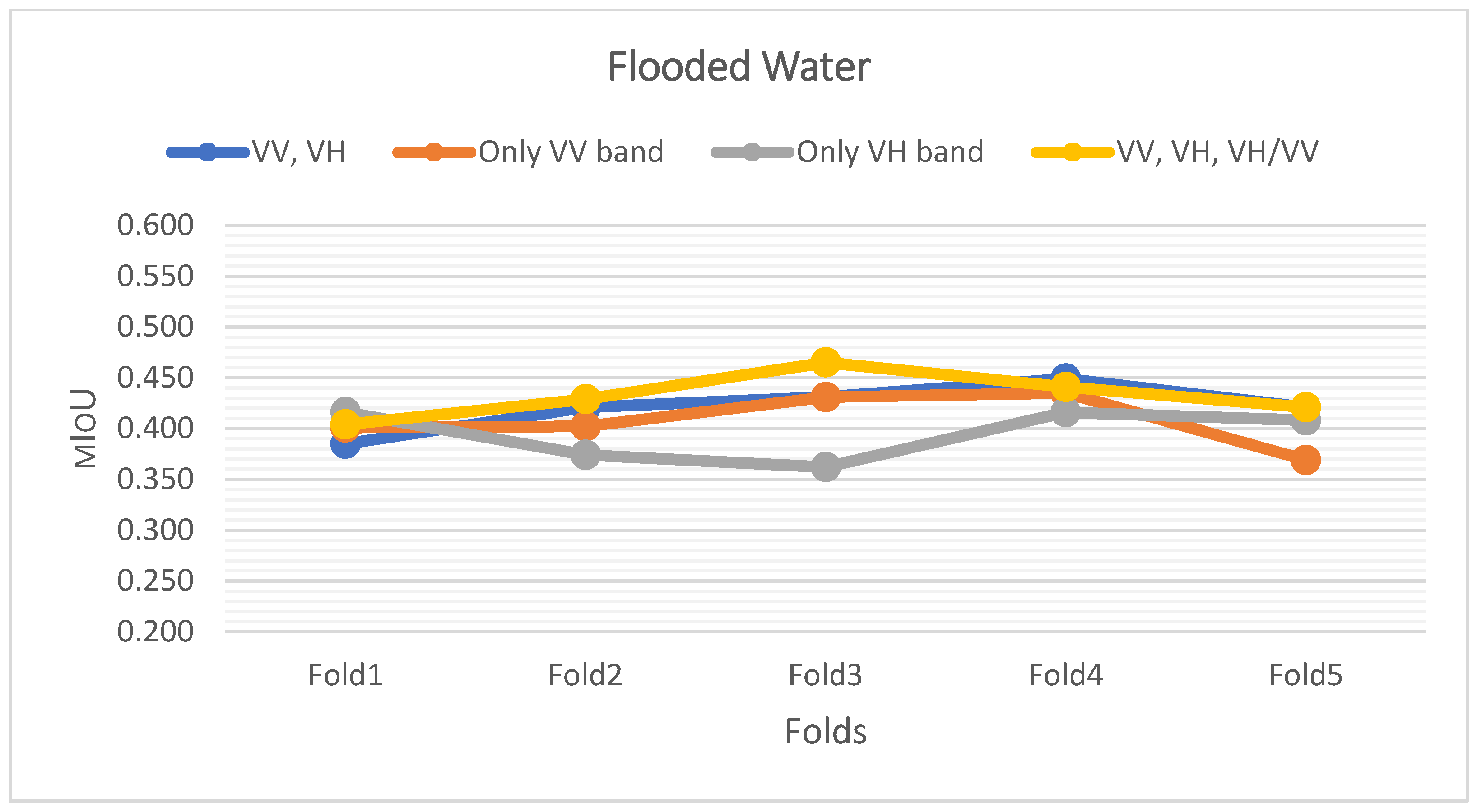
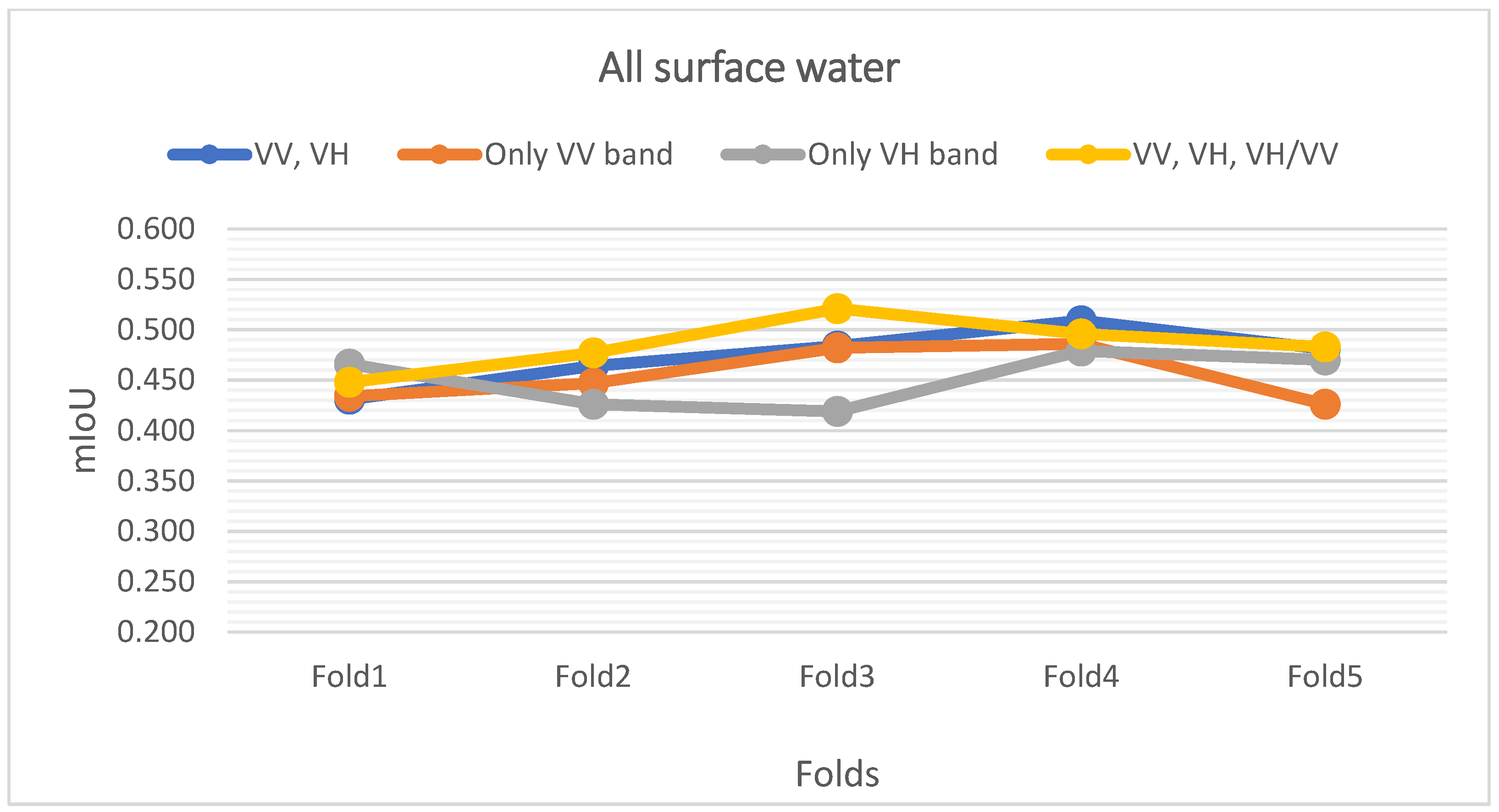
Appendix A. K-Fold Cross-Validation Result

To investigate the generalization capability of the model as well as to ensure that model is not overfitting on the given data, K-fold cross-validation was used. For the implementation we have used hand-labeled data. First dataset has been divided into five equal parts or folds, and then four model for each band combination has been trained by leaving one part for testing and using four parts for training. This way we have trained five sets of models by leaving different part as a test set in every time, to cover the whole dataset. The result of the models against the permanent water, flooded water and all-surface water is shown in Figure A1, Figure A2 and Figure A3. The average of all five models with each band combination is mentioned in Figure A1 along with the standard deviation. Results suggest that our models are consistent throughout different folds with standard deviation ranging between 2–4%.
Figure A1. Model’s performance with permanent water extraction case.
Remotesensing 13 02334 g0a1
Figure A2. Model’s performance with flooded water extraction case.
Remotesensing 13 02334 g0a2
Figure A3. Model’s performance with all surface water extraction case.
Remotesensing 13 02334 g0a3
Table A1. Performance of the models over 5-fold.
Permanent WaterFlooded WaterAll Surface Water
Band UsedAverage
mIoU
Std. Dev.Average
mIoU
Std. Dev.Average
mIoU
Std. Dev.
VV, VH0.5240.0400.4210.0210.4730.026
Only VV band0.4740.0390.4070.0240.4540.025
Only VH band0.5140.0330.3950.0230.4510.025
VV, VH, VV/VH0.5110.0390.4320.0200.4840.024

References

  1. UNEP Goal 11: Sustainable Cities and Communities. Available online: https://www.unep.org/explore-topics/sustainable-development-goals/why-do-sustainable-development-goals-matter/goal-11 (accessed on 16 January 2021).
  2. Yang, H.; Wang, Z.; Zhao, H.; Guo, Y. Water body extraction methods study based on RS and GIS. Procedia Environ. Sci. 2011, 10, 2619–2624. [Google Scholar] [CrossRef] [Green Version]
  3. Huang, C.; Chen, Y.; Zhang, S.; Wu, J. Detecting, extracting, and monitoring surface water from space using optical sensors: A review. Rev. Geophys. 2018, 56, 333–360. [Google Scholar] [CrossRef]
  4. Schumann, G.J.P.; Moller, D.K. Microwave remote sensing of flood inundation. Phys. Chem. Earth 2015, 83, 84–95. [Google Scholar] [CrossRef]
  5. Xu, H. Modification of normalised difference water index (NDWI) to enhance open water features in remotely sensed imagery. Int. J. Remote Sens. 2006, 27, 3025–3033. [Google Scholar] [CrossRef]
  6. Feyisa, G.L.; Meilby, H.; Fensholt, R.; Proud, S.R. Automated water extraction index: A New technique for surface water mapping using landsat imagery. Remote Sens. Environ. 2014, 140, 23–35. [Google Scholar] [CrossRef]
  7. Yang, X.; Qin, Q.; Grussenmeyer, P.; Koehl, M. Urban surface water body detection with suppressed built-up noise based on water indices from sentinel-2 MSI imagery. Remote Sens. Environ. 2018, 219, 259–270. [Google Scholar] [CrossRef]
  8. Herndon, K.; Muench, R.; Cherrington, E.; Griffin, R. An Assessment of surface water detection methods for water resource management in the Nigerien sahel. Sensors 2020, 20, 431. [Google Scholar] [CrossRef] [PubMed] [Green Version]
  9. Feng, W.; Sui, H.; Huang, W.; Xu, C.; An, K. Water Body Extraction from very high-resolution remote sensing imagery using deep U-Net and a superpixel-based conditional random field model. IEEE Geosci. Remote Sens. Lett. 2019, 16, 618–622. [Google Scholar] [CrossRef]
  10. Schumann, G.J.P.; Brakenridge, G.R.; Kettner, A.J.; Kashif, R.; Niebuhr, E. Assisting flood disaster response with earth observation data and products: A critical assessment. Remote Sens. 2018, 10, 1230. [Google Scholar] [CrossRef] [Green Version]
  11. Assad, S.E.A.A. Flood Detection with a Deep Learning Approach Using Optical and SAR Satellite Data. Master’s Thesis, Leibniz University Hannover, Hannover, Germany, 2019. [Google Scholar]
  12. Rambour, C.; Audebert, N.; Koeniguer, E.; le Saux, B.; Crucianu, M.; Datcu, M. Flood detection in time series of optical and SAR images. Int. Arch. Photogramm. Remote Sens. Spat. Inform. Sci. 2020, 43, 1343–1346. [Google Scholar] [CrossRef]
  13. Bioresita, F.; Puissant, A.; Stumpf, A.; Malet, J.P. Fusion of sentinel-1 and sentinel-2 image time series for permanent and temporary surface water mapping. Int. J. Remote Sens. 2019, 40, 9026–9049. [Google Scholar] [CrossRef]
  14. Shen, X.; Anagnostou, E.N.; Allen, G.H.; Robert Brakenridge, G.; Kettner, A.J. Near-real-time non-obstructed flood inundation mapping using synthetic aperture radar. Remote Sens. Environ. 2019, 221, 302–315. [Google Scholar] [CrossRef]
  15. Huang, X.; Wang, C.; Li, Z. A near real-time flood-mapping approach by integrating social media and post-event satellite imagery. Ann. GIS 2018, 24, 113–123. [Google Scholar] [CrossRef]
  16. Landuyt, L.; van Wesemael, A.; Schumann, G.J.P.; Hostache, R.; Verhoest, N.E.C.; van Coillie, F.M.B. Flood mapping based on synthetic aperture radar: An assessment of established approaches. IEEE Trans. Geosci. Remote Sens. 2019, 57, 722–739. [Google Scholar] [CrossRef]
  17. Hostache, R.; Matgen, P.; Wagner, W. Change detection approaches for flood extent mapping: How to select the most adequate reference image from online archives? Int. J. Appl. Earth Obs. Geoinform. 2012, 19, 205–213. [Google Scholar] [CrossRef]
  18. Otsu, N. A threshold selection method from gray-level histograms. IEEE Trans. Syst. Man Cybern 1979, 9, 62–66. [Google Scholar] [CrossRef] [Green Version]
  19. Kittler, J.; Illingworth, J. Minimum error thresholding. Pattern Recognit. 1986, 19, 41–47. [Google Scholar] [CrossRef]
  20. Martinis, S.; Twele, A.; Voigt, S. Towards operational near real-time flood detection using a split-based automatic thresholding procedure on high resolution TerraSAR-X data. Nat. Hazards Earth Syst. Sci. 2009, 9, 303–314. [Google Scholar] [CrossRef]
  21. Zhang, P.; Chen, L.; Li, Z.; Xing, J.; Xing, X.; Yuan, Z. Automatic extraction of water and shadow from SAR images based on a multi-resolution dense encoder and decoder network. Sensors 2019, 19, 3576. [Google Scholar] [CrossRef] [PubMed] [Green Version]
  22. Katiyar, V.; Tamkuan, N.; Nagai, M. Flood area detection using SAR images with deep neural. In Proceedings of the 41st Asian Conference of Remote Sensing—Asian Association of Remote Sensing, Deqing, China, 9–11 November 2020. [Google Scholar]
  23. Bonafilia, D.; Tellman, B.; Anderson, T.; Issenberg, E. Sen1Floods11: A georeferenced dataset to train and test deep learning flood algorithms for sentinel-1. In Proceedings of the IEEE Computer Society Conference on Computer Vision and Pattern Recognition Workshops, Seattle, WA, USA, 14–19 June 2020; pp. 835–845. [Google Scholar] [CrossRef]
  24. Li, Y.; Martinis, S.; Wieland, M.; Schlaffer, S.; Natsuaki, R. Urban flood mapping using SAR intensity and interferometric coherence via bayesian network fusion. Remote Sens. 2019, 11, 2231. [Google Scholar] [CrossRef] [Green Version]
  25. Twele, A.; Cao, W.; Plank, S.; Martinis, S. Sentinel-1-based flood mapping: A fully automated processing chain. Int. J. Remote Sens. 2016, 37, 2990–3004. [Google Scholar] [CrossRef]
  26. Clement, M.A.; Kilsby, C.G.; Moore, P. Multi-temporal synthetic aperture radar flood mapping using change detection. J. Flood Risk Manag. 2018, 11, 152–168. [Google Scholar] [CrossRef]
  27. Tiwari, V.; Kumar, V.; Matin, M.A.; Thapa, A.; Ellenburg, W.L.; Gupta, N.; Thapa, S. Flood inundation mapping-Kerala 2018—Harnessing the power of SAR, automatic threshold detection method and Google Earth engine. PLoS ONE 2020, 15, e0237324. [Google Scholar] [CrossRef]
  28. Caballero, I.; Ruiz, J.; Navarro, G. Sentinel-2 satellites provide near-real time evaluation of catastrophic floods in the west mediterranean. Water 2019, 11, 2499. [Google Scholar] [CrossRef] [Green Version]
  29. Sekou, T.B.; Hidane, M.; Olivier, J.; Cardot, H. From patch to image segmentation using fully convolutional networks—Application to retinal images. arXiv 2019, arXiv:1904.03892. [Google Scholar]
  30. Goodfellow, I.; Bengio, Y.; Courville, A. Deep Learning; MIT Press: Cambridge, MA, USA, 2016; ISBN 3463353563306. [Google Scholar]
  31. Badrinarayanan, V.; Kendall, A.; Cipolla, R. Segnet: A deep convolutional encoder-decoder architecture for image segmentation. IEEE Trans. Pattern Anal. Mach. Intell. 2017, 39, 2481–2495. [Google Scholar] [CrossRef] [PubMed]
  32. Ronneberger, O.; Fischer, P.; Brox, T. U-Net: Convolutional networks for biomedical image segmentation. Lect. Notes Comput. Sci. 2015, 9351, 234–241. [Google Scholar] [CrossRef] [Green Version]
  33. Wang, J.; Sun, K.; Cheng, T.; Jiang, B.; Deng, C.; Zhao, Y.; Liu, D.; Mu, Y.; Tan, M.; Wang, X.; et al. Deep high-resolution representation learning for visual recognition. IEEE Trans. Pattern Anal. Mach. Intell. 2020. [Google Scholar] [CrossRef] [Green Version]
  34. Fu, J.; Liu, J.; Tian, H.; Li, Y.; Bao, Y.; Fang, Z.; Lu, H. Dual attention network for scene segmentation. In Proceedings of the IEEE/CVF Conference on Computer Vision and Pattern Recognition, Long Beach, CA, USA, 15–20 June 2019; pp. 3146–3154. [Google Scholar]
  35. Bahl, G.; Daniel, L.; Moretti, M.; Lafarge, F. Low-power neural networks for semantic segmentation of satellite images. In Proceedings of the International Conference on Computer Vision Workshop, ICCVW, Seoul, Korea, 27 October–2 November 2019; pp. 2469–2476. [Google Scholar] [CrossRef] [Green Version]
  36. Jadon, S. A Survey of loss functions for semantic segmentation. In Proceedings of the IEEE Conference on Computational Intelligence in Bioinformatics and Computational Biology (CIBCB), Viña del Mar, Chile, 27–29 October 2020. [Google Scholar] [CrossRef]
  37. Kingma, D.P.; Ba, J.L. Adam: A method for stochastic optimization. In Proceedings of the 3rd International Conference on Learning Representations (ICLR 2015—Conference Track Proceedings), San Diego, CA, USA, 7–9 May 2015; pp. 1–15. [Google Scholar]
  38. Li, L.; Yan, Z.; Shen, Q.; Cheng, G.; Gao, L.; Zhang, B. Water body extraction from very high spatial resolution remote sensing data based on fully convolutional networks. Remote Sens. 2019, 11, 1162. [Google Scholar] [CrossRef] [Green Version]
  39. Huang, Z.; Pan, Z.; Lei, B. What, where, and how to transfer in SAR target recognition based on deep CNNs. IEEE Trans. Geosci. Remote Sens. 2020, 58, 2324–2336. [Google Scholar] [CrossRef] [Green Version]
  40. Flores-Anderson, A.I.; Herndon, K.E.; Thapa, R.B.; Cherrington, E. Sampling designs for SAR-assisted forest biomass surveys. In The SAR Handbook—Comprehensive Methodologies for Forest Monitoring and Biomass Estimation; SAR: Santa Fe, NM, USA, 2019; pp. 281–289. [Google Scholar] [CrossRef]
  41. Manjusree, P.; Prasanna Kumar, L.; Bhatt, C.M.; Rao, G.S.; Bhanumurthy, V. Optimization of threshold ranges for rapid flood inundation mapping by evaluating backscatter profiles of high incidence angle SAR Images. Int. J. Disaster Risk Sci. 2012, 3, 113–122. [Google Scholar] [CrossRef] [Green Version]
  42. Yosinski, J.; Clune, J.; Bengio, Y.; Lipson, H. How transferable are features in deep neural networks? Adv. Neural Inf. Process. Syst. 2014, 4, 3320–3328. [Google Scholar]
  43. Schmitt, M. Potential of large-scale inland water body mapping from sentinel-1/2 data on the example of Bavaria’s lakes and rivers. PFG J. Photogramm. Remote Sens. Geoinf. Sci. 2020, 88, 271–289. [Google Scholar] [CrossRef]
Figure 1. Kerala district map showing the areas worst affected by the 2018 flood.
Remotesensing 13 02334 g001
Figure 2. Network representations. (a) SegNet-like network and (b) UNet-like network.
Remotesensing 13 02334 g002
Figure 3. Details of the selected area from the test site. (a) Sentinel-2 composite image in false color (B12-B8-B4). (b) Created validation flood mask (blue and white color represents water and non-water areas correspondingly), (c,d) descending and ascending SAR images of the area of interest, respectively.
Remotesensing 13 02334 g003
Figure 4. mIoU of the SegNet models trained with different band combinations over all three training sets.
Remotesensing 13 02334 g004
Figure 5. mIoU of the UNet models trained with different band combinations over all three training sets.
Remotesensing 13 02334 g005
Figure 6. Merged SAR (VH band) image and the corresponding combined result of both Otsu thresholding (OT) and deep learning (DL) method in a single image. White and black pixels in the resulting image represent pixels detected by both algorithms as either water or non-water, respectively. Whereas, red and cyan pixels show the difference in both the algorithms. Cyan pixels imply, that area was classified as water by DL but as non-water by OT and just the opposite in the case of red pixels.
Remotesensing 13 02334 g006
Table 1. Characteristics of the Sentinel-1 and Sentinel-2 images used for the test area.
Satellite Image NameAcquisition Date (yyyy/mm/dd)Flight DirectionProcessing Level
S1A_IW_GRDH_1SDV_20180821T004109_20180821T004134_023337_0289D5_B2B22018/08/21DescendingL1-GRD (IW)
S1A_IW_GRDH_1SDV_20180821T130602_20180821T130631_023345_028A0A_C7282018/08/21AscendingL1-GRD (IW)
S1A_IW_GRDH_1SDV_20180821T004044_20180821T004109_023337_0289D5_D07A2018/08/21DescendingL1-GRD (IW)
S1A_IW_GRDH_1SDV_20180821T130631_20180821T130656_023345_028A0A_E1242018/08/21AscendingL1-GRD (IW)
S2B_MSIL1C_20180822T050649_N0206_R019_T43PFL_20180822T0851402018/08/22DescendingLevel 1C
Table 2. Performance of different SegNet models over all the test cases (bold text represents the best result).
SegNet/Dataset and Band UsedPermanent WaterFlooded WaterAll Surface Water
mIoUOm.Comm.mIoUOm.Comm.mIoUOm.Comm.
Sentinel-1 weak labels
VV, VH0.4920.0080.0460.2860.3780.0440.3640.2490.044
Only VV band0.5190.2550.0320.2380.4740.0370.3130.3970.037
Only VH band0.4820.0090.0480.2820.3820.0490.3590.2510.049
VV, VH, VH/VV0.5150.0110.0430.2810.410.0420.3600.2690.043
Sentinel-2 weak labels
VV, VH0.4690.0080.0240.3420.3650.0210.4170.2390.020
Only VV band0.4840.3150.0210.2920.4340.0160.3570.3930.016
Only VH band0.4830.0060.0250.3180.3820.0210.3960.2520.020
VV, VH, VH/VV0.5340.0140.0180.3150.4380.0140.3920.2900.014
Hand labelling
VV, VH0.4470.0050.0290.3470.3410.0240.4210.2230.024
Only VV band0.4630.2850.0310.3420.3550.0230.4120.3310.023
Only VH band0.4630.0110.0320.2960.4290.0210.3740.2830.021
VV, VH, VH/VV0.4840.0070.0240.3360.4040.0190.4110.2650.019
Benchmark from [23]
Otsu thresholding0.4570.0540.0850.2850.1510.0850.3590.1430.085
Baselines from [23]
Sentinel-1 weak labels (VV, VH)0.2870.0660.1350.2420.1190.1000.3090.1120.997
Sentinel-2 weak labels (VV, VH)0.3820.1210.0530.3390.2680.0780.4080.2480.078
Hand labeling (VV, VH)0.2570.0950.1520.2420.1350.1060.3130.1300.106
Table 3. Performance of different UNet models over all the test cases.
UNet/Dataset and Band UsedPermanent WaterFlooded WaterAll Surface Water
mIoUOm.Comm.mIoUOm.Comm.mIoUOm.Comm.
Sentinel-1 weak labels
VV, VH0.4060.0060.0520.2880.3520.0500.3490.2310.050
Only VV band0.4850.2850.0350.2570.4450.0380.3320.3890.038
Only VH band0.4570.0080.0210.2850.3900.0430.3620.2560.043
VV, VH, VH/VV0.4460.0060.0390.2750.3960.0370.3530.2590.037
Sentinel-2 weak labels
VV, VH0.5290.0090.0170.3660.3580.0140.4390.2360.014
Only VV band0.4270.2930.0210.3030.4020.0190.3670.3640.019
Only VH band0.4690.0040.0250.3320.3620.0210.4070.2360.021
VV, VH, VH/VV0.4580.0040.0290.3620.3130.0240.4340.2050.024
Hand labelling
VV, VH0.3860.0050.0420.3610.2740.0350.4320.1810.035
Only VV band0.3860.2890.0380.3390.3150.0290.4040.3060.029
Only VH band0.4360.0050.0350.3090.3630.0290.3860.2360.029
VV, VH, VH/VV0.4620.0030.0270.3590.3090.0240.4360.2020.024
Benchmark from [23]
Otsu thresholding0.4570.0540.0850.2850.1510.0850.3590.1420.085
Baseline from [23]
Sentinel-1 weak labels (VV, VH)0.2870.0660.1350.2420.1190.1000.3090.11240.997
Sentinel-2 weak labels (VV, VH)0.3820.1200.0530.3390.2680.0780.4080.24820.078
Hand labeling (VV, VH)0.2570.0940.1520.2420.1350.1050.3120.12970.105
Table 4. Results of the transfer learning performed using hand-labeled data on the UNet model trained on Sentinel-2 weakly labeled data with both polarizations (bold text represents the best result).
Transfer Learning/DatasetPermanent WaterFlooded WaterAll Surface Water
mIoUOm.Comm.mIoUOm.Comm.mIoUOm.Comm.
Hand labelling
Whole model0.5300.00510.02640.4090.34940.02070.4830.22870.0207
Whole decoder0.5310.00540.03240.3660.37450.02380.4430.24510.0238
Whole encoder0.5320.00410.02430.4200.30860.02040.4940.20420.0204
Otsu thresholding (OT)0.4570.0540.08490.2850.1510.08490.35910.14270.0849
% improvement over OT+16.4−92.4−71.37+47.3+104.3−75.9+37.6+43.1−75.9
Table 5. Evaluation of the different methods on the test site (bold text represents the best result).
MethodImagesIoUF1 ScoreOm. ErrorComm. Error
Minimum and Otsu thresholdingMerged images of ascending flight direction0.83940.91270.13280.0367
Our model (after transfer learning)Merged images of ascending flight direction0.88490.93890.05870.0635
Minimum and Otsu thresholdingMerged images of descending flight direction0.82140.90190.15350.0347
Our model (after transfer learning)Merged images of descending flight direction0.87760.93480.06610.0642
Publisher’s Note: MDPI stays neutral with regard to jurisdictional claims in published maps and institutional affiliations.

