Article

Automatic Point Cloud Semantic Segmentation of Complex Railway Environments

1
Centro de Investigación en Tecnoloxías, Enerxía e Procesos Industriais (CINTECX), Applied Geotechnologies Research Group, Campus Universitario de Vigo, Universidade de Vigo, As Lagoas, Marcosende, 36310 Vigo, Spain
2
Department of Cartographic and Terrain Engineering, University of Salamanca, Calle Hornos Caleros 50, 05003 Avila, Spain
*
Author to whom correspondence should be addressed.
Remote Sens. 2021, 13(12), 2332; https://doi.org/10.3390/rs13122332
Submission received: 14 April 2021 / Revised: 7 June 2021 / Accepted: 11 June 2021 / Published: 14 June 2021

Abstract

:
The growing development of data digitalisation methods has increased their demand and applications in the transportation infrastructure field. Currently, mobile mapping systems (MMSs) are one of the most popular technologies for the acquisition of infrastructure data, with three-dimensional (3D) point clouds as their main product. In this work, a heuristic-based workflow for semantic segmentation of complex railway environments is presented, in which their most relevant elements are classified, namely, rails, masts, wiring, droppers, traffic lights, and signals. This method takes advantage of existing methodologies in the field for point cloud processing and segmentation, taking into account the geometry and spatial context of each classified element in the railway environment. This method is applied to a 90-kilometre-long railway lane and validated against a manual reference on random sections of the case study data. The results are presented and discussed at the object level, differentiating the type of the element. The indicators F1 scores obtained for each element are superior to 85%, being higher than 99% in rails, the most significant element of the infrastructure. These metrics showcase the quality of the algorithm, which proves that this method is efficient for the classification of long and variable railway sections, and for the assisted labelling of point cloud data for future applications based on training supervised learning models.

Graphical Abstract

1. Introduction

Transport infrastructures are massively used around the globe for several purposes such as passenger or freight transport, being vitally important to society. Among the various modes of transport, the most used ones are roads and railways. In 2018, the use of road and railway services for freight transport was 1.2 million and 250 thousand tonne-kilometre (tkm) in the EU, and 7.12 million and 2.88 million tkm in China [1]. In addition to freight transportation, rail and road infrastructures also have relevant importance in passenger transport. In this respect, the use of road services was 3.5 trillion passenger-kilometre (pkm) in the EU and almost 1 trillion in China and Japan. The use of railways was 380 billion in the EU, 400 billion in Japan, and 1.4 trillion pkm in China. These data indicate the huge use and consequently the importance of the infrastructures in our society.
Considering the relevance of the infrastructures, safety is an aspect of critical importance. In the EU, only on railways, there were 1763 accidents in 2015, with 930 fatalities. Moreover, 31 accidents involved the transport of dangerous goods [2].
Recently, concern about increasing the safety of railway infrastructures has risen. This, together with technological advances, has allowed the development of algorithms to digitise infrastructures. Building information modelling (BIM) is one of the solutions mostly used [3], considerably increasing the efficiency of the industry by improving the interoperability and the integration of the information of large construction projects [4]. In the field of railways, Biancardo et al. present a procedural modelling-based BIM approach for railway design, discussing different BIM-based tools depending on the design requirements, such as OpenSCAD or Rhinoceros [5]. In this respect, Bansalah et al. present an integration of BIM in a railway project with the advantages of serving as decision support and control of the phases during the development of the project, and as assistance for maintenance once completed [6].
However, the geometric model design of the existing infrastructure may not be straightforward to replicate in a BIM-oriented framework. Thus, several techniques are being developed, based on remotely sensed data, to digitise the as-is geometric information of the infrastructure. These techniques aim for a high level of automatisation, reducing the manual operation both in the acquisition phase and in the processing phase, and improving the safety of workers. In the field of road infrastructures, previous work presents a semi-automated method to define the alignment of road infrastructure following the Industry Foundation Classes (IFCs) standard, thus aiming for an interoperable definition of the infrastructure valid for a BIM methodology. This method is able to generate the alignment from 3D point cloud data by detecting the road edges based on the intensity level of the road markings [7]. In the field of railway infrastructures, Cheng et al. present an automatic creation of as-is building information models from railway tunnel point clouds [8], implementing an algorithm to segment the cloud based on their characteristics and distribution in tunnels, generating parametric models of the elements based on the estimated railway alignments and creating a BIM model using an application based on the software MicroStation [9]. This approach is promising, but it only addresses a specific part of the railway infrastructure.
One of the most widespread technologies used to gather accurate data on infrastructures is mobile laser scanning (MLS). There are a vast number of studies showing the capabilities of this technology in the field of road and rail infrastructures [10,11,12,13,14]. It can be inferred that MLS technology is able to generate representations of the environment in the form of 3D point clouds. However, the raw data are unstructured; thus, the development of point cloud segmentation and classification algorithms is necessary to identify and locate different elements required for the digitalisation of the infrastructure. Aside from MLS, there are different types of sensors, such as the type used by Qiang Han et al. to analyse the fastener in rail tracks [15]. That sensor consists of combining a 3D depth image with a 2D intensity image. Grzegorz Gabara et al. present an approach for railway track inspection using a digital single-lens reflex (DSLR) camera to generate image-based point clouds [16]. However, since these photogrammetric methods generate structured data, the computational cost is higher than using MLS in the case of recording linear structures (such as railway infrastructures). Regardless, a segmentation and classification process is required to extract the information of the data.
According to this, several authors have developed algorithms to automatically segment railway point clouds. Zhu et al. analyse airborne and mobile laser scanning point clouds, recognising objects surrounding railway infrastructure but do not analyse the infrastructure itself [17]. Yang et al. use geometry and intensity data to analyse railway MLS points clouds, but they only focus on rail track recognition [18]. Elberink et al. present a method to extract and model rail track centrelines [19]. They apply local properties, such as height and parallelism, to extract roughly the rail tracks, refining the results with a modelling process. However, other elements are not analysed. Arastounia implements a segmentation process based on PCA to segment wiring points, using a region growing algorithm to group them. However, this algorithm does not consider proximity between wires as their data only have one railway track [20]. In previous research, an automatic detection method is presented, along with the decomposition of a railway from cloud points in tunnels, with good results using support vector machine algorithms (SVMs), but it is not applicable to more complex and variable scenarios [21]. In other previous studies, [22] a different method is introduced with the same objectives, using Pointnet [23] and KPConv [24], but applicable only to tunnels. In that vein, a methodology is developed that is applicable to complex areas and tested at 90 km but only for the delineation of railway lanes in order to generate IFC alignment models [25].
As a follow-up to those studies, this paper aims to introduce an algorithm that improves existing point cloud segmentation methods in railway environments, presenting the following contributions:
(1)
It offers a complete segmentation of the railway environment, including rails, masts, wiring, droppers, traffic lights, and signals. Slab tracks were not considered a relevant item when the objectives of this project were discussed;
(2)
It is applied to a 90 km long railway scenario, showing its versatility and ability to be generalised to different scenarios such as tunnels, as well as to complex areas with a variable number of railway lanes.
This work is structured as follows: first, the case study is presented in Section 2. Then, Section 3 details the developed methodology for the segmentation of the railway environment using 3D point cloud data. Then, the method is evaluated in Section 4. Finally, Section 5 and Section 6 present a discussion of the method and its results and the conclusions of this study, respectively.

2. Case Study

The scenario used to validate the methodology presented in this paper consists of 90 km of railway section shown in Figure 1, surveyed with an average speed of 10 km/h. This scenario has been acquired in May 2019 using the LYNX Mobile Mapper by Optech [26], a system using two LiDAR sensors. The specifications of the sensors can be found in [27]. For computational reasons, the complete dataset is divided into 450 georeferenced point clouds in .las format, thus averaging a length of 200 m for each individual point cloud. The dataset contains more than 3000 million points, being considerably larger than in other state-of-the-art works.
Moreover, the path followed by the sensor, its trajectory, is also used. The attributes of this trajectory are spatial location and time stamp.

3. Methodology

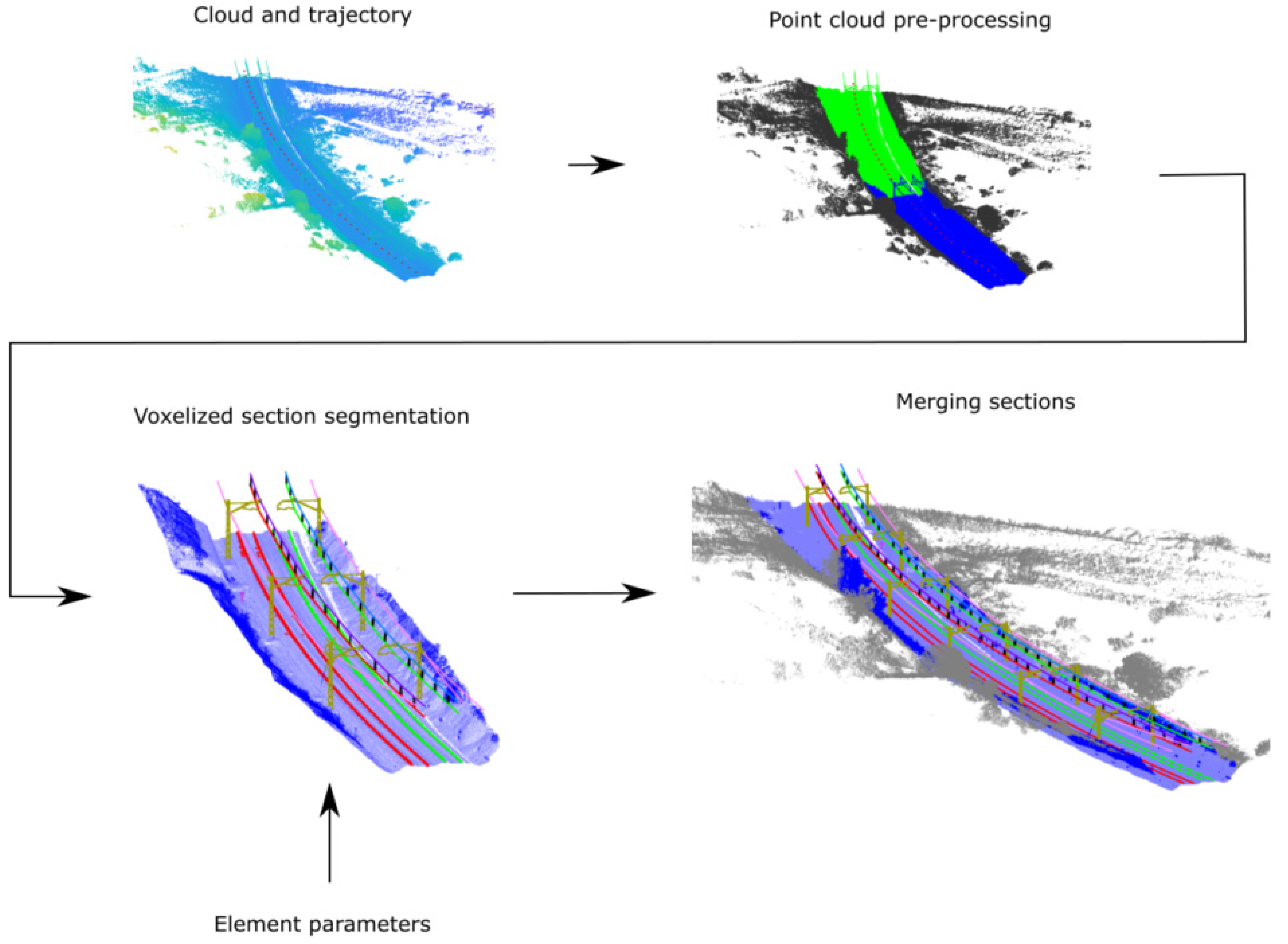
This paper presents an automatic heuristic segmentation of railway point clouds. A schematic representation of the methodology is shown in Figure 2. The methodology consists of a preprocessing step, in which each point cloud is sectioned and voxelised; a segmentation process, through which each voxelised section is segmented; a merging process, through which the segmented sections are regrouped into the whole dataset.

3.1. Point Cloud Preprocessing

The input data consist of 450 point clouds as well as the trajectory of the sensor during the survey. Let an individual point cloud be C i = ( x ,   y ,   z ,   I ,   t s ) , an N p × 5 matrix where ( x ,   y ,   z ) are the coordinates, I the intensity, and t s the timestamp of the N p points. Furthermore, let the trajectory be T = ( x ,   y ,   z ,   t s ) , an N t × 4 matrix where ( x ,   y ,   z ) are the coordinates as recorded by the navigation system, and t s is a timestamp which is synchronised with the point cloud data.
These point clouds are raw data, neither organised nor adapted to be directly segmented. Therefore, it is necessary to apply preprocessing algorithms to simplify the data, making the segmentation process lighter and more effective. To that end, a sectioning process, followed by a voxelisation process, is applied to each point cloud C i .

3.1.1. Sectioning

During the survey, the complete railway environment is captured, i.e., the infrastructure as well as other elements such as vegetation, constructions, or slopes. Consequently, a significant portion of the point clouds does not provide relevant information. Furthermore, the railway curvature effect and the variable length of the infrastructure, presented in each C i , also increase the complexity of the segmentation process.
Taking this into account, a sectioning algorithm is applied to reduce the size of the input data. Sectioning preprocesses are commonly used in these kinds of scenarios by other authors such as in [20]. This preprocessing algorithm consists of splitting C i in sections, limiting their length and curvature, and only including points related to the infrastructure, removing points that would only include noise and computational load to the segmentation process.
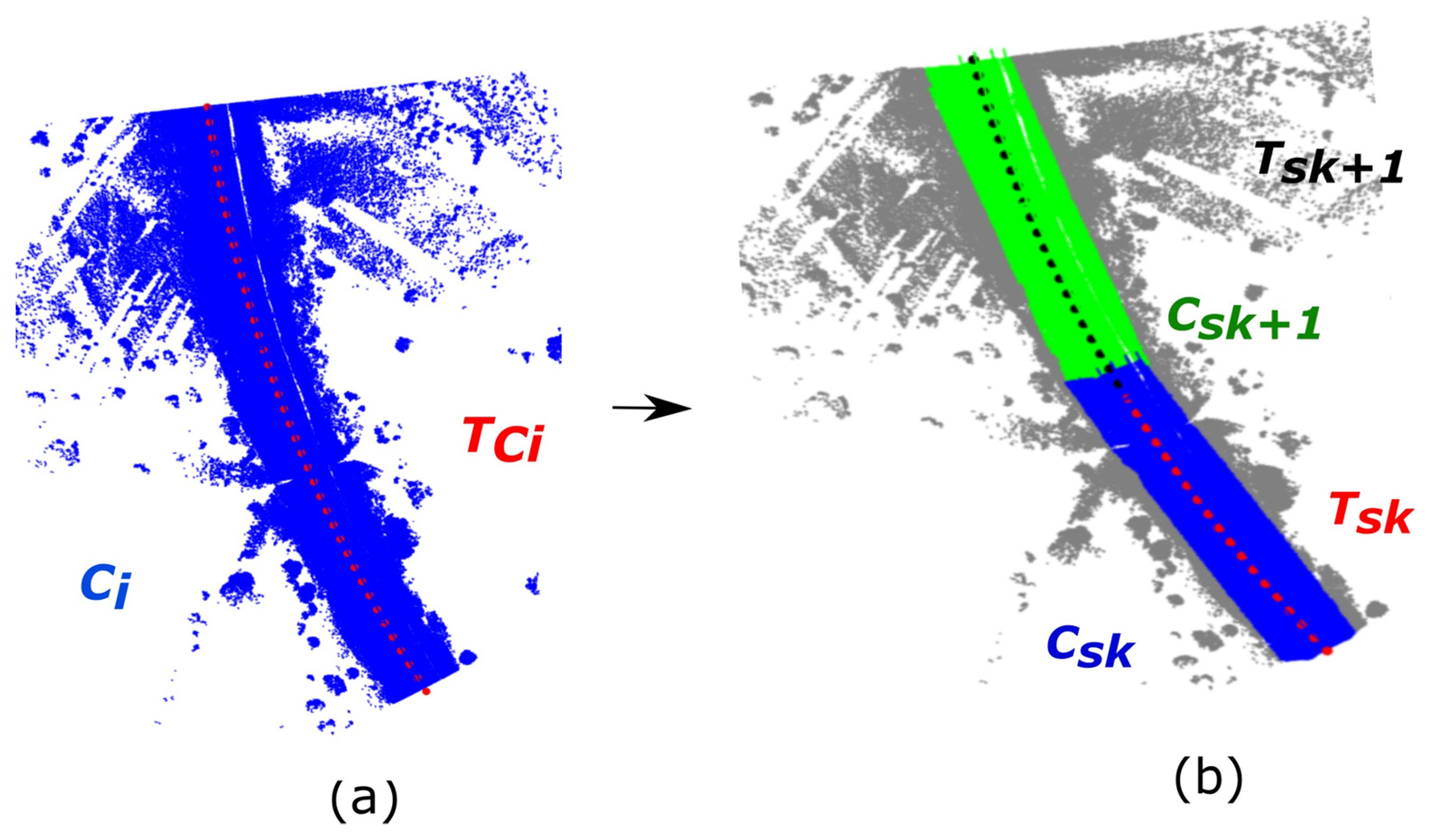
This process starts by splitting T into sections, which are used later to divide each C i . As the trajectory T covers the complete dataset, it is necessary to know which portion of T overlaps with each C i . To that end, the following three steps are applied for each C i : (1) points in T with a timestamp within the range of C i timestamp [ t i m e   s t a m p   m a x ,   t i m e   s t a m p   m i n ] are selected; (2) points in T outside of C i bounding box are removed; (3) the closest points in C i to the first and last points of the selected T slice are selected. Then, the closest points in T to those C i points are classified as the first and the last points of the T slice for the cloud under study. Let the selected T points corresponding to C i be T C i (Figure 3a).
Next, T C i is sectioned in slices with a length equal to l s , and each resulting section is defined as T s k . This length is calculated as the distance between the first and last point of each slice. Then, a modified principal component analysis (MPCA) is applied to T s k . MPCA works as follows: Let the reference axes be X 0 ,   Y 0 ,   Z 0 , being Z 0 a vector perpendicular to the Earth plane pointing upwards. Let A be a set of points. Let the eigenvectors of principal components obtained by applying principal component analysis (PCA) to A be X p c a ,   Y p c a ,   Z p c a , sorted into descending order by its correspondent eigenvalues. Let the result of applying MPCA to A be the axes X m p c a ,   Y m p c a ,   Z m p c a . The origin of these axes is A ¯ , where ¯ denotes a mean operator. The construction of the vector base X m p c a is made by assigning it to X p c a , Y m p c a orthogonal to the X p c a and parallel to the X 0 Y 0   plane, and Z m p c a = ± ( X m p c a     Y m p c a   ) with the Z -component restricted to be positive.
For performing spatial operations, coordinates on the reference axes X 0 ,   Y 0 ,   Z 0 of a point P = P X 0 , P Y 0 , P Z 0 can be expressed in X p c a ,   Y p c a ,   Z p c a axes. These operations are a translation and a rotation, as shown in Equation (1).
P X m p c a , P Y m p c a , P   Z   m p c a =   ( P X 0 , P Y 0 , P Z 0   A ¯ X 0 ,   A ¯ Y 0 , A ¯ Z 0 )     X p c a Y p c a   Z p c a
A representation of this process is shown in Figure 2.
The aim of applying MPCA instead of PCA is to calculate a reference system in which the set of points are oriented but not rotated in its main direction (Figure 4). Let the resulting directions after applying MPCA to T s k be X ,   Y ,   Z . Considering the MPCA operations, X is the direction of the trajectory in T s k , and Y is the direction perpendicular to the trajectory and parallel to the X 0 Y 0 plane. If X ,   Y ,   Z was the result of applying PCA instead of MPCA, the Y direction might not be parallel to X 0 Y 0 if T s k were too straight. It is interesting that the Y direction is parallel to this plane, which is the ground plane, when using it for measuring distances to the rail track.
Once X ,   Y ,   Z axes are calculated, T s k curvature is evaluated as follows: if T s k range interval in the Y direction, [ T s k   Y   m i n , T s k   Y   m a x ] , is greater than c u r s , which means that the effect of the curvature is too high for segmentation purposes. In those cases, T s k is redefined by iteratively removing its last point, making the segment shorter until the curvature effect is under the threshold c u r s . Once T s k is defined, the next section T s ( k + 1 ) starts in the last point that was removed for the calculation of T s k (Figure 3b). This process is applied until all points in T C i belong to a T s k section. As a result, the trajectory T is sectioned in such a way that each individual point cloud C i has one or many T s k trajectory sections.
After T is split into sections T s k , each C i cloud is sectioned accordingly, generating a set of C s k sections. The first step consists of calculating the coordinates of C i points in X ,   Y ,   Z axes. For computational reasons, not all C i points are recalculated. When T s ( k 1 )   is calculated, C i points with an X lower than T s ( k 1 )   X   m a x are not considered in the following sections. Additionally, points with a timestamp greater than T s k   t s   m a x + ( T s k   t s   m a x T s k   t s   m i n ) are also removed. In this way, C i points from previous sections out of the overlap area are not considered, and only C i points corresponding to T s k including a safety margin are taken into account. Finally, the points assigned to the section under study are the ones with a | Y | < w s , and X < T s k   X   m a x + o v s . This removes points that are both far from the infrastructure and after the last T s k point in the X direction. However, it adds a certain overlap area, o v s , including points in this section that are also included in the next one. The overlap simplifies the process of linking linear elements after the segmentation process.
A schematic representation of the sectioning process is shown in Figure 3.

3.1.2. Voxelisation

The sectioning is a preprocess applied to the raw data in order to properly prepare it for a segmentation process by generating smaller sections of the data. Nevertheless, the point cloud data is still unstructured and not homogeneous; hence, a voxelisation is proposed to achieve the following objectives:
  • Homogenising the cloud, i.e., allowing density-based analyses with no influence on the distance between the studied area and the sensor;
  • Knowing the neighbourhood of each voxel, i.e., it is useful in the segmentation process to know the local properties of each voxel;
  • Reducing the number of points, i.e., making the process faster and reducing the computational load. The impact of this reduction is driven by the voxel size g v .
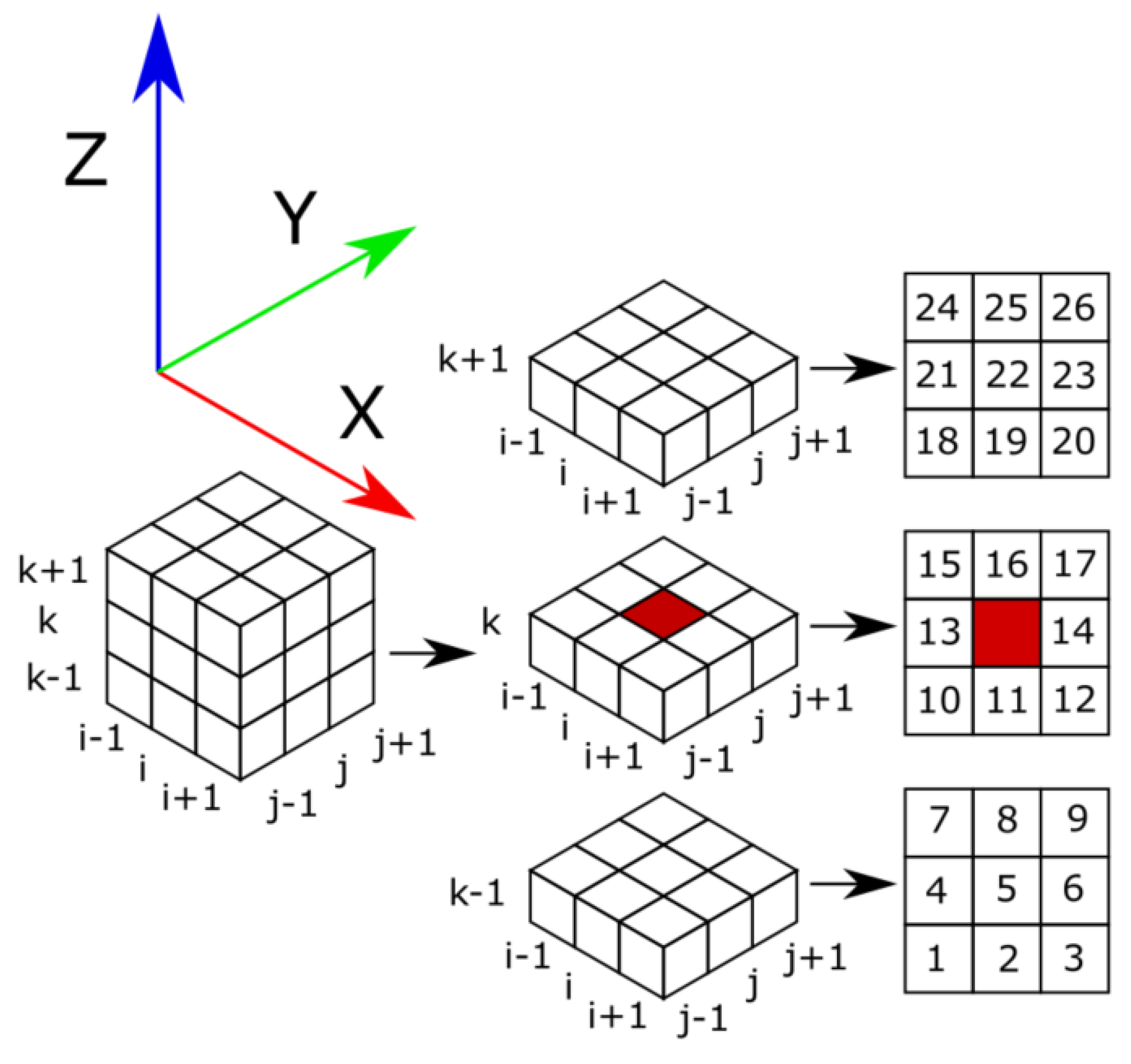
Chen et al. define a voxelised object as a “3D discrete representation of a continuous object on a regular grid of voxels” [28]. The process of voxelisation in 3D is an analogous process to the rasterisation process in 2D. This process consists of discretising the space in a regular grid of boxes. These boxes, called voxels, are 3D elements analogous to pixels. Several features can be analysed in voxels based on the points contained in them or their distribution in the space. In this work, since the objective is to segment different elements in point clouds, the coordinates of each voxel are calculated as the centroid of the points contained in each voxel. Furthermore, empty voxels are not stored in memory. Moreover, since it is a regular grid, the spatial distribution of the voxels is known, having a unique index which identifies them. Hence, the neighbourhood of each voxel is known. Figure 5 shows a representation of the voxel’s neighbourhood with the notation used in this paper. According to this notation, if voxel i is just above voxel j , i is neighbour 22 of voxel j , and j is neighbour 5 of voxel i .
This voxelisation process is applied to all C s k from the same C i joined. In this way, only one voxelisation operation is needed for each C i . The voxelised cloud is referred to as V i , and its sections corresponding to each C s k are V s k .

3.2. Point Cloud Segmentation

Once the data are organised to be segmented, the algorithms explained in this section are applied. The main objective of this segmentation process is the extraction of the railway track, masts, wiring, droppers, signage elements, and rails from each point cloud C i .
The input to this process is V s k , with voxel coordinates calculated in X ,   Y ,   Z axes, resulting from the application of MPCA to its corresponding T s k .

3.2.1. Railway Track

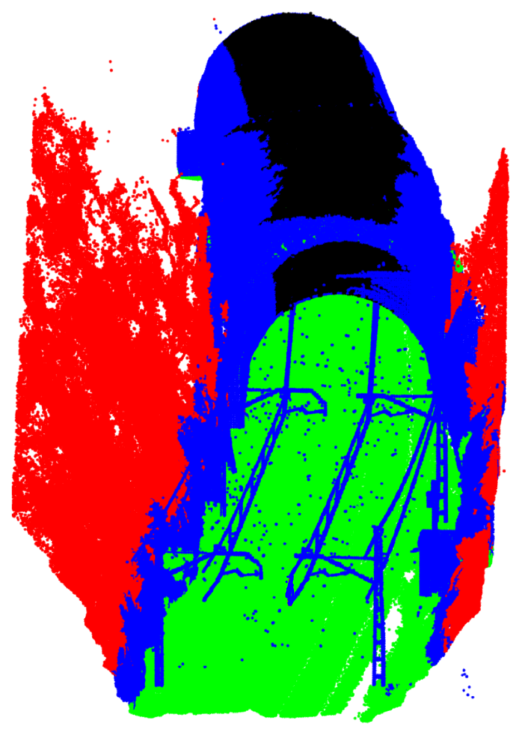
The track is the part of the railway infrastructure that contains the rails, ballasts, sleepers, and all the elements on the ground that are relevant to the infrastructure. On the other hand, the infrastructure components that are not on the track are over it. These spatial considerations facilitate the segmentation of the railway track when applying different algorithms that take into account the position of the infrastructure components with respect to the track. Other authors, such as those in [20], take these same considerations into account to perform a track segmentation step. Figure 6 shows the results of this process on a voxelised point cloud V s k , once the following process is applied:
  • Voxelisation: this is performed with a voxel grid greater than the rail height, as rails will be considered part of the railway track. Let the voxel size and the resulting voxelised cloud be g v B and V s k , respectively.
  • Track extraction: with an adequate definition of g v B , it can be assumed that track voxels in V b s k do not have neighbours, neither just above them nor under them (neighbours 5 and 22 in Figure 5). Accordingly, voxels that comply with that criteria are selected. Then, neighbouring voxels whose Euclidean distance is less than c l t are clustered, filtering out clusters with less than p t voxels. Then, voxels in clusters positioned under the trajectory T s k are segmented as track voxels. Finally, voxels with any neighbour in the same height level (neighbours 10–17) segmented as track are also considered as track voxels. The voxels in V b s k segmented as track are referred to as V b t . The correspondent voxels in V s k are referred to as V t .
  • Peripherical voxels extraction: voxels from the track limits in the Y direction are segmented as peripherical voxels, as these voxels do not have relevant information about the infrastructure. To do so, V b s k is split into sections perpendicularly to the X axis, with a width s t t . In each section, the Y limits of V b t are calculated, and the voxels out of those margins, plus a small distance, r m t , are segmented as peripherical voxels. The voxels in V s k segmented as peripherical voxels are referred to as V p . It is important to note that this step is not applied in the sectioning process. There, the filter used in the direction perpendicular to the trajectory in the ground plane considers the distance to the trajectory. However, this process considers the limits of the railway track as obtained in the previous step, which are variable depending on the presence of walls, vegetation, or other types of built obstacles.
  • Overpass extraction: at this point of the process a local principal component analysis is applied in order to analyse the local dimensionality of the point cloud. First, voxels which meet [ V t ¯     V p ¯ ] are selected. Then, PCA is applied to each selected voxel considering a neighbourhood that includes voxels whose Euclidean distance is less than d 1 from it. Since overpasses are planar elements with a vertical normal vector, voxels with a Z component in its third eigenvector greater than e v t r are selected. Then, neighbouring voxels whose Euclidean distance is less than c l t are clustered, and groups with less than p r voxels are removed. Finally, voxels in the selected clusters are segmented as lining voxels. Overpass extraction is necessary because wiring and overpass are so close that it causes interferences in the wiring segmentation algorithm if overpasses are not previously removed. The highest part of tunnel linings is also segmented as an overpass. The voxels in V s k segmented as lining voxels are referred to as V o .

3.2.2. Masts

This step of the process aims to segment those voxels that belong to masts. In the same way as for overpass and lining segmentation, a local principal component analysis is applied, considering, in this case, all the voxels in [ V t ¯     V p ¯ ] . First, PCA is applied to each selected voxel considering a neighbourhood that includes voxels whose Euclidean distance is less than d 2 from it. Let the eigenvectors obtained at the voxel i be v 1 ,   v 2 , v 3 . Let the normalised principal components deviations at voxel i be λ 1 ,   λ 2 , λ 3 . The mast extraction process is divided into the following steps, the workflow process of which is represented in Figure 7:
  • Voxels with v 1   Z > m z , v 1   X < m x , and v 1   Y < m y are selected. The objective is the detection of voxels whose neighbourhood has a vertical dispersion. Then, its neighbours are added. This is necessary because masts are not isolated since they are in contact with wires. Figure 7a shows the selected voxels.
  • The selected voxels are clustered using DBSCAN [29], considering c l m distance and at least one voxel per cluster. Then, clusters that do not meet the “Mast without cantilever” model specifications are removed. Figure 7b shows the selected clusters.
  • Voxels close to each cluster are added to complete the mast. The centroids of the selected clusters define the centres of the masts, but they might be incomplete. Therefore, all the voxels within the dimensional specifications of the “Mast without cantilever” model with respect to the centre of the mast are selected, except for the voxels in V t , which are not part of the mast segments. Then, those voxels are clustered again using DBSCAN with the same parameters as in the previous step. Next, the voxels of the cluster which shares most voxels with the cluster of the mast are added to that mast. Figure 7c shows the voxels added to each mast.
  • Once the mast segmentation process without cantilevers is performed, they are added. Voxels with v 1   X < m c z and X > 0 are selected and grouped using DBSCAN (same parameters as before) and discarding voxels in V p . The objective is the detection of voxels whose neighbourhood has no dispersion in the trajectory direction. Figure 7d shows the selected voxels.
  • Then, clusters in contact with any mast are added to them as their cantilever. Figure 7e shows the masts and the cantilevers.
  • Finally, after wiring extraction, which is presented in Section 3.2.3, masts that are not in contact with any wire are deleted. The voxels classified as masts without cantilever are referred to as V r m , and those classified as masts with cantilever as V m .

3.2.3. Wiring

This phase of the process aims to segment those voxels that belong to wires. The first step is based on the same concept as for masts extraction: applying local PCA. However, since wires are smaller than masts, it is necessary to apply local PCA to all the voxels that are in [ V t ¯     V p ¯ ] considering a smaller neighbourhood: d 1 . Consequently, the eigenvectors v 1 ,   v 2 , v 3 and corresponding eigenvalues λ 1 ,   λ 2 , λ 3 obtained from PCA are recalculated.
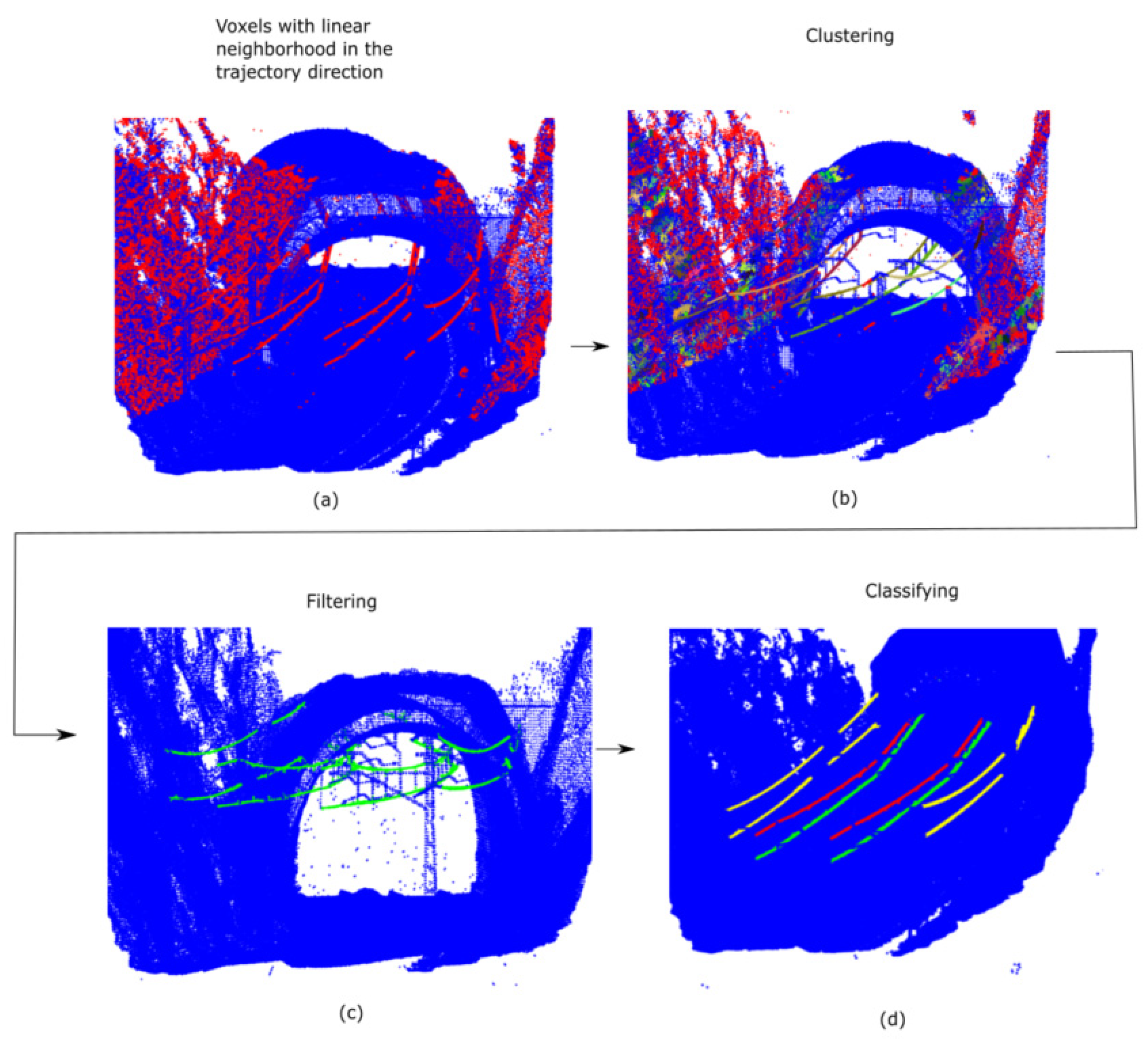
This process is implemented as follows, the workflow of which is shown in Figure 8:
  • Selecting voxels with v 1   X > w x and X > 0 in [ V t ¯     V m ¯ ] : In this way, voxels whose neighbourhood has its main dispersion in the trajectory direction are selected. An example is shown in Figure 8a.
  • Clustering: wiring voxels cannot be clustered either by distance or by neighbourhood because they can be in contact with each other; hence, they are grouped together. Moreover, wire voxels in contact with masts are segmented as masts, and therefore, this clustering would cause breakups in wire clusters. Consequently, a different cluster algorithm is applied considering the wiring casuistry. This algorithm is based on the proposed process in [30], which is a region growing algorithm that guides the growing areas. However, the following modification is applied: each cluster has a seed that is the voxel which define the starting point for the region growing of its cluster. The point cloud formed by the selected voxels is split into sections perpendicularly to the X axis. The width of each section is equal to s t w . Each section is analysed by order, assigning its voxel to a cluster existing in a previous section or making a new cluster. Distances between the voxels in the section under study and the seeds of the clusters in the previous sections are calculated. Each voxel is assigned to the cluster of its closest seed in Y if this distance is lower than the width of the wire, specified by the “Wire” model. The voxels that are not assigned to any cluster are grouped using DBSCAN. The wire width is used as distance, which is specified by the “Wire” model with at least one cluster per voxel; this process forms new clusters. Once the section is analysed, the seeds are updated. The new seed of each cluster is the closest voxel in this section to the seed of its cluster, measured in Y . In a new cluster, the seed is its central voxel. Those clusters that do not have propagation do not update their seed. Lastly, seeds in which the distance to the section under study is greater than d i s t w are removed; hence, their cluster does not grow anymore. An example is shown in Figure 8b.
  • Filtering clusters: the objective is to remove clusters that are not wires. Three considerations are made, namely, (1) a minimum wire longitude l w ; (2) λ 1 ¯ > λ w , rejecting clusters that are not linear elements; (3) a minimum density equal to d w , avoiding noise such as vegetation. An example is shown in Figure 8c.
  • Classifying wires as catenary, contact, or others: in a railway infrastructure, a contact wire has a catenary wire over it. From a bird’s eye view, contact and catenary wires share the same positions (they lay in the same projection on the ground). In order to do this analysis, the clusters are rasterised, applying an orthonormal projection in the   X Y plane. As a result of this rasterisation, a digital image is obtained, retaining the information of which voxels are contained in each pixel. The size of the pixels is set to 2 3   m s w . With this image, each cluster is studied independently. For each cluster, adjacent pixels in the horizontal direction are added to make it wider. In this way, it is considered a range search equal to m s w from the wire. After that, pixels that contain voxels of the wire under study and voxels of the other wires are evaluated. The wire with the highest percentage of shared pixels, measured in the shorter of both, is classified as its couple only if this percentage is greater than p e r w . A couple of wires is formed by a contact wire and the catenary wire over it. Then, the Z ¯ of each wire and its couple is calculated, considering only the voxels corresponding to the pixels that the wires have in common. The wire with the highest Z ¯ is classified as catenary; otherwise, it is classified as contact wire. Additionally, considering that a wire might be wrongly classified as several wires, those wires with the same couple are grouped since they must be the same wire. Nevertheless, verification is necessary after the droppers’ extraction: contact–catenary couples must have droppers between them. Droppers are the element that joins catenary and contact wires. Finally, clusters that are neither catenary nor wire are classified as other wires only if they are in contact with any mast. Otherwise, their voxels are not segmented as wires. An example is shown in Figure 8d. The voxels classified as wires are referred to as V w .

3.2.4. Droppers

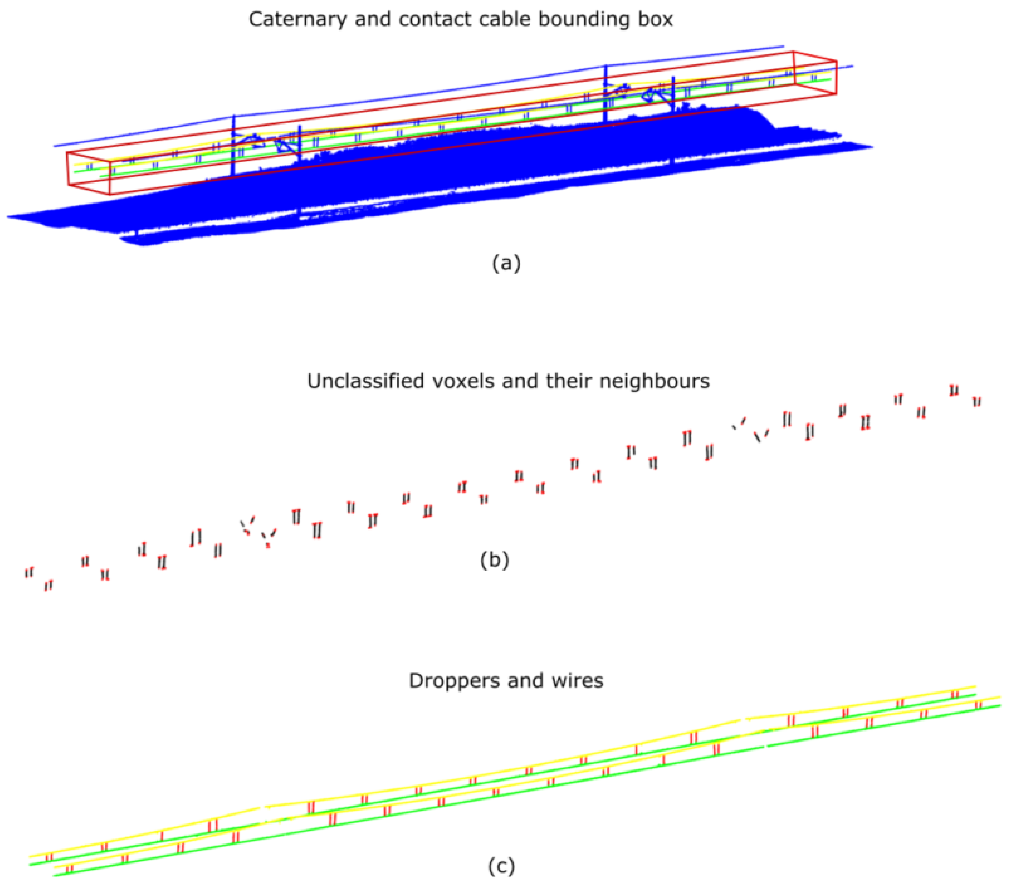
This step aims to segment droppers using the previous results. Droppers are the element that joins catenary and contact wires. A schematic representation of this process is shown in Figure 9. Dropper segmentation process works as follows:
  • Voxels inside the bounding box of contact and catenary wires in [ V t ¯     V m ¯       V w ¯ ] are selected. Figure 9a shows this step.
  • Neighbours of the selected voxels are added. This step aims to include voxels of catenary and contact wires that are in contact with droppers. Figure 9b shows an example with the selected voxels and their neighbours.
  • Clustering is performed using DBSCAN, considering c l d distance and at least one cluster per voxel.
  • Clusters that do not have common voxels with any pair of contact–catenary wiring are removed. They must have common voxels with both wires. Moreover, clusters that do not meet the “Dropper” model specifications are also removed.
  • Lastly, selected clusters are classified as droppers, removing V w . Each dropper voxel is associated with a cluster and each cluster with a catenary–contact pair. An example with the classified droppers is shown in Figure 9c. The voxels classified as droppers are referred to as V d .

3.2.5. Signage Elements

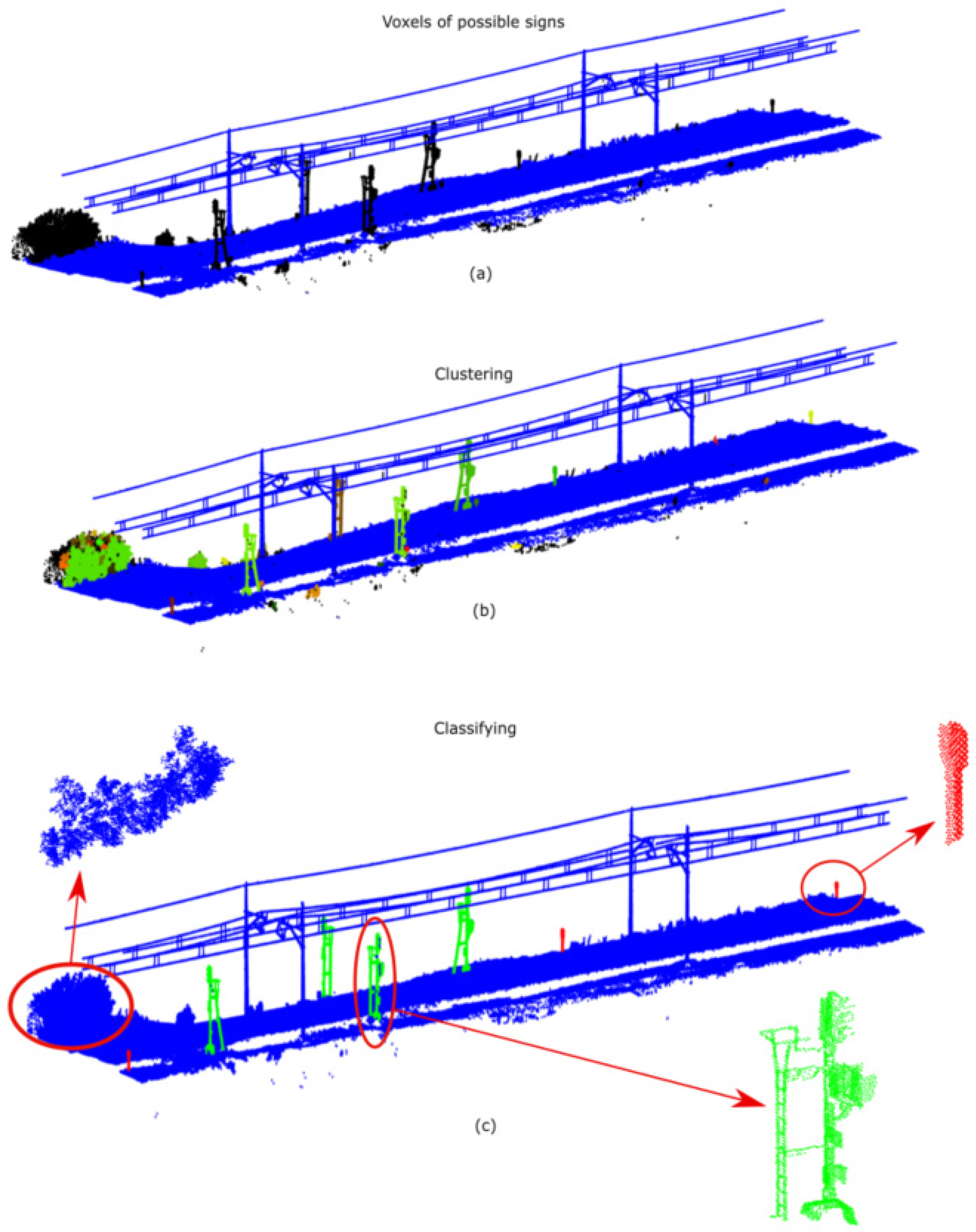
In contrast to the methods explained above, which aim to segment elements that are in contact with others, this sign segmentation process aims to segment isolated elements. Thus, voxels in [ V t ¯     V m ¯       V w ¯       V d ¯ ] are selected. Then, neighbouring voxels whose Euclidean distance is less tan c l s are clustered. Next, clusters with any voxel from V p are removed. This process is shown in Figure 10a.
These clusters are classified as traffic signs, traffic lights, or marks if meeting the specifications of “Sign”, “Traffic Light”, or “Mark” model, respectively. To have more resolution, points from C i in each cluster are retrieved from their voxels and compared with the models. However, since their coordinates have not been modified, they are referred to as X ,   Y ,   Z axis. This process is shown in Figure 10b.
As it is shown in Table 1, some models consider distances between the point cloud of the model and the element under study. To do this process correctly, they must be centred on the same point. For this reason, the centre of coordinates of each cluster is modified by applying Equation (2) to the points of the element under study. It allows the points centred in its centre of mass to be represented in the X Y directions, setting its highest point to Z = 0 . This results in an easier comparison, avoiding problems with poles of variable length. The point cloud of the model is the centre in the same way. This process is shown in Figure 10c.
P i   x '     P i   y '   P i   z ' = P i   x     P i   y   P i   z P x ¯     P y ¯   P z   m a x
The specifications of the models are applied in the following order, and the selected cluster has to meet all of them:
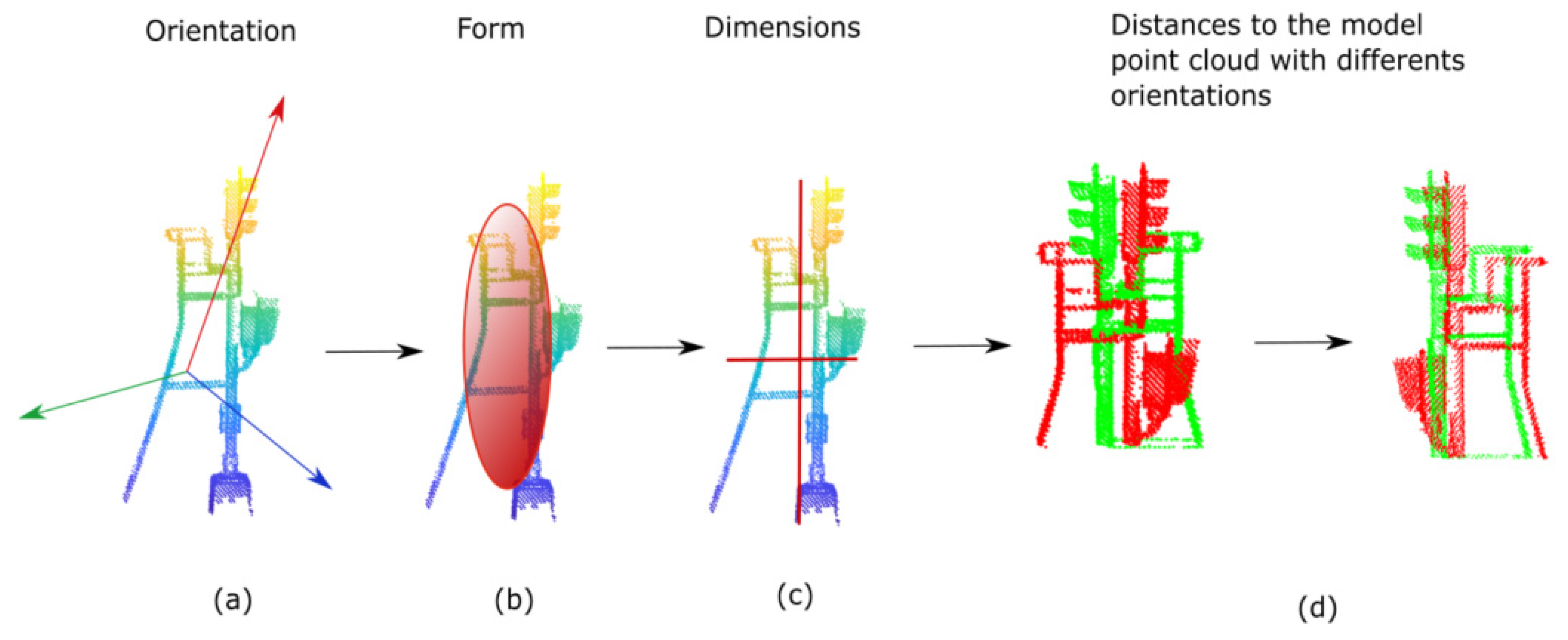
  • Orientation: this is defined by the eigenvectors obtained by applying PCA to the cluster and the specified ones. Its deviation to the model is measured as the angle between these eigenvectors and the vectors of the model. This process is shown in Figure 11a.
  • Shape: it includes the normalised eigenvalues. Its process is shown in Figure 11b.
  • Dimensions: first, they are measured as the ranges of the cluster in the X Y Z directions. If the element does not meet the required tolerance, they are measured in their eigenvector’s directions. In other words, if the ranges do not meet with the element oriented using the trajectory, it is oriented using its own dimensionality. The range parameter considered in each new dimension is the range parameter of their principal X Y Z direction. It is necessary because some signage elements may be slightly tilted in their principal direction. This process is shown in Figure 11c.
  • Similitude with a template point cloud: this similitude is evaluated as the distance between the clouds, calculated as shown in Equation (3), being A the n points of the model and B the m points of the cluster under study. These distances are measured using k-nearest neighbours [31]. The point clouds of the models only include the highest part of the signs, with a small part of the pole. Consequently, points under study below the lowest point of the model are not included. Moreover, signage elements might be oriented in opposite directions. Hence, if the cluster does not meet the distance specification, it is rotated 180° on axis   Z . If it still does not meet the requirement, the same process is repeated by orienting the cluster using its eigenvector’s directions, following the same reasoning as in the previous step. This process is shown in Figure 11d.
    d i s t a n c e = m a x ( d i s t a n c e s ( A , B ) 2 ¯ , d i s t a n c e s ( B , A ) 2 ¯ )
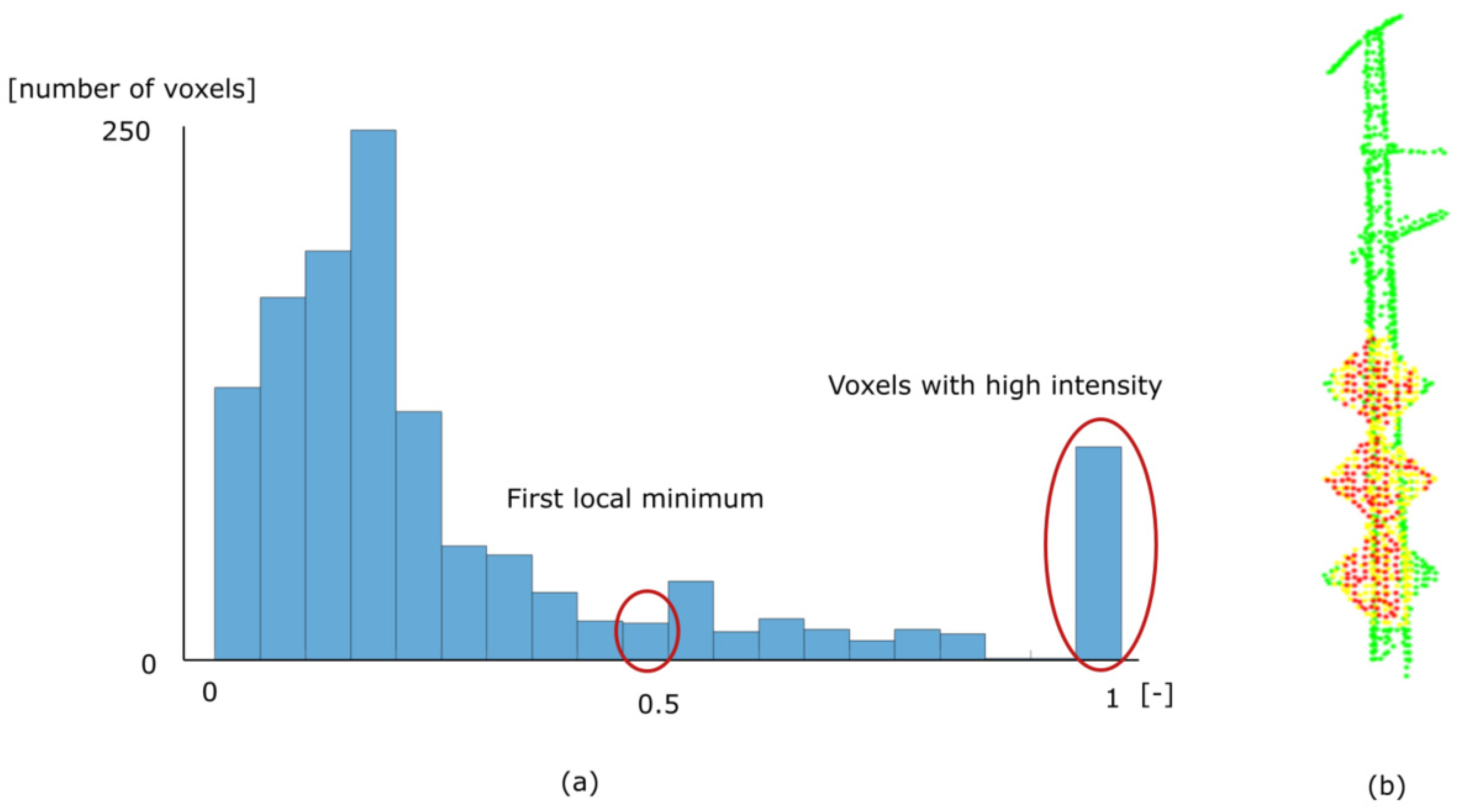
The segmentation of signs that are hung from masts has also to be considered, and it follows a different process. As these signs are made of retroreflective materials, the intensity attribute of their points is clearly distinguishable from their surroundings. Accordingly, this process analyses each mast as segmented in Section 3.2.2, normalising the intensity values of their voxels. An intensity histogram with h s bins is computed. If the percentage of voxels in the last bin is greater than p s i g , it means that there are signs in that mast. In that case, the first local minimum in the histogram is calculated. Then, voxels in the bins with an intensity higher than the first local minimum are clustered. Next, clusters with less than p r voxels are discarded. Finally, the voxels in the selected clusters and their neighbours are segmented as signs on that mast. Figure 12 shows segmented signs on a mast and their normalised intensity histogram.

3.2.6. Rails

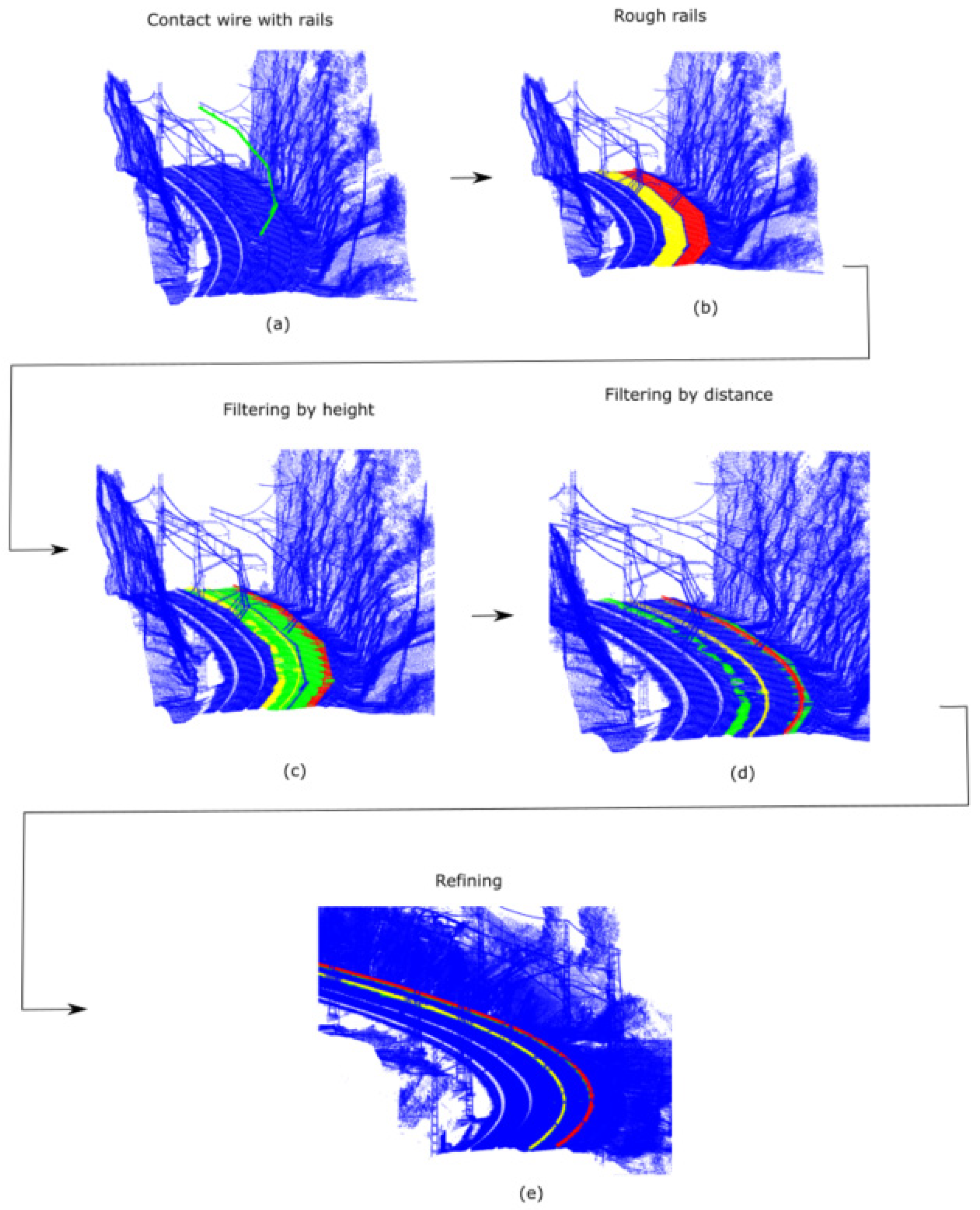
Currently, different rail segmentation algorithms developed based on changes in the track height have been developed [32,33]. However, because of the track irregularity, slopes along the railway may cause false positives, and irregularities in the ballast distribution might produce false negatives. Consequently, in order to avoid those errors, this method uses contact wiring as reference for the segmentation of the rails. The contact wire position with respect to the rail is constant; therefore, it is used to make a rough approximation of the position of both rails. In addition, this allows a semantic relationship between contact wires and rails to be assigned. Thus, this algorithm assigns a rails pair to each catenary–contact wiring couple. It is implemented as follows, with the schematic workflow process shown in Figure 13:
  • Contact wire with rails under it: since wires start and end in a mast but not the rails, it is necessary to verify which portion of the wire is over the rails. A contact wire does not have rails under it from its last contact with a cantilever to its contact with a mast. Additionally, in that part of the wire, there are no droppers. Consequently, the ends of the wire are analysed. If they are in contact with a mast or there are no droppers between them and its closest cantilever, that wire part is not considered for rail segmentation purposes. This process is shown in Figure 13a.
  • Rough rails: V s k is rasterised, applying an orthonormal projection in   X Y plane. Pixels corresponding to the segment of the wire with rails are selected. Then, the digital image is analysed column by column (moving forward along the X axis) selecting pixels at both sides of wire pixels where rails are supposed to be, knowing the distance between one rail and its pair, and also knowing that the contact wire is in the middle of both. This distance is defined by the “Pair of rails” model. To obtain a rough segmentation of the rails, pixels at a distance less than m s r from the pixels where the rail is supposed to be are also included. The right and left pixels are organised separately. Next, voxels corresponding to the selected pixels and segmented as V t are chosen. These voxels contain rails and their surroundings.
  • Filtering each rough rail by height individually: each rail is analysed individually, applying MPCA to orient and section it in the rail direction, with s t r as the section width. Then, a histogram of Z coordinates in each section is computed. The largest bin is considered the ground height. Therefore, voxels with a lower Z coordinate are removed.
  • Filtering the pair of rails by distance: in order to remove false negatives caused by irregularities in the track, voxels that do not have the rail pair at the right distance are removed. This process is performed in the digital image. The image is analysed column by column (moving forward along X axis), saving pixels that have any pixel of its rail pair at the correct distance. Voxels corresponding to those pixels are segmented as rails.
  • Refining rails: As rails are continuous elements always in contact with the track, it is not possible to determine their limits in V s k with a voxel size g v . Hence, after the merging section process. shown in Section 3.3, C i points corresponding to the extracted voxels are denoised. Each rail is individually analysed. Their points are oriented using MPCA and sectioned in the direction of the rails, with s t r as the section width. Then, a Y histogram is computed in each section detecting the largest bin, its width being b r . The Y of the largest bin is the average Y of the rail. Then, points whose distance in Y to that position is lower than rails width are selected. Finally, track points are removed by deleting points with a lower Z than the mean Z of the selected voxels.

3.3. Merging Sections

The processes described above are applied to each V s k in such a way that each V s k is segmented as an independent cloud. This process aims to merge the sections and obtain the indices of points in the original clouds C i corresponding to the segmented voxels. The indices of the elements segmented correspond to their V s k , and therefore, they are recalculated, obtaining the indices corresponding to its V i . Then, the merging process consists of comparing the elements in V s k with the elements in V s ( k 1 ) until the last section, saving the indices of new elements and classifying them as the same element where applicable. This process distinguishes three types of elements: points, continuous elements, and elements dependent on continuous elements.
Point elements are analysed individually. An element in V s k is added only if none of its voxels are at any element of the same type in V s ( k 1 ) . This step is necessary because there may be an overlap between sections.
Continuous elements are the contact wires, catenary, and other wires. The objective is to determine which elements in V s k are the continuation of the elements segmented in V s ( k 1 ) . To that end, each element in V s k is compared with the elements of the same type in V s ( k 1 ) . The distances from the first voxel of the element under study to the last voxels of the elements in V s ( k 1 ) are measured. To be merged, these distances in X and Y must be lower than m s x and m s y , respectively. If there are several elements that meet these requirements, it is assigned to the wire with more common voxels (there is overlap between sections). If there is a tie, it is assigned to the wire with less distance in Y . In the case of contact–catenary pair, it is only considered the one which best meets the requirements.
Dependent elements of continuous elements are rails and droppers. These elements are joined to their correspondent contact–catenary pair.
Finally, C i element indices are extracted from V s indices as the points inside each voxel.
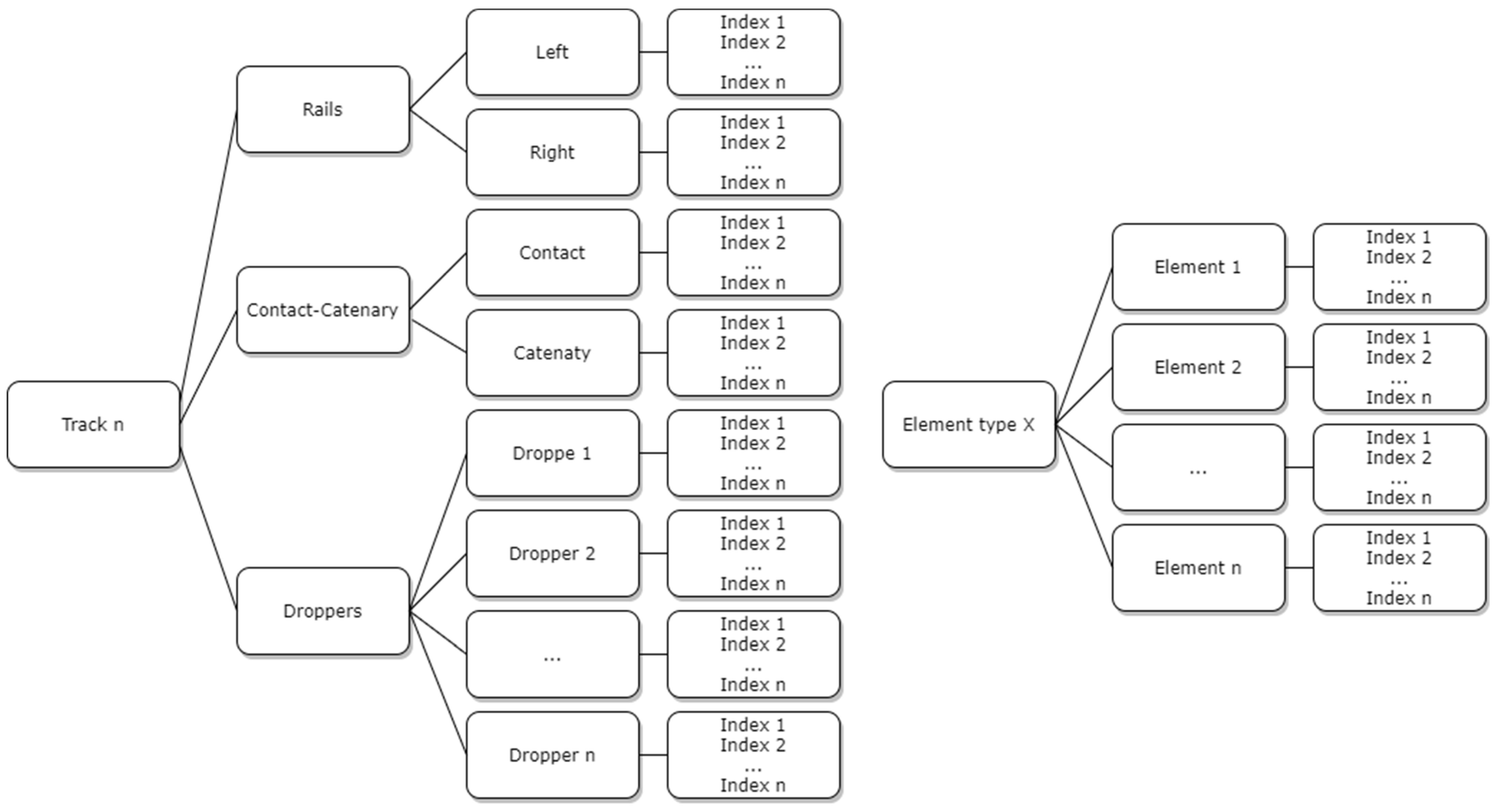
As a result, the information obtained after applying the segmentation process is not organised by sections. For each C i , the indices of each element are grouped, identifying the type of element. Moreover, elements belonging to the same track, such as contact wires, catenary wires, rails, and droppers, are grouped together in the same structure. Figure 14 shows how the segmentation obtained is organised.

4. Results

This section shows the results from the application of the defined methodology to the case study data. Moreover, this section also describes the process used to validate the methodology.
First, it is important to introduce the values of the parameters used throughout the processes described in Section 3. Some of these parameters are based on previous knowledge of the geometry of railway infrastructure and its assets, while others have been adjusted empirically. Their values are shown in Table 2. Then, Table 1 shows the specifications of the geometry models used in the segmentation process.
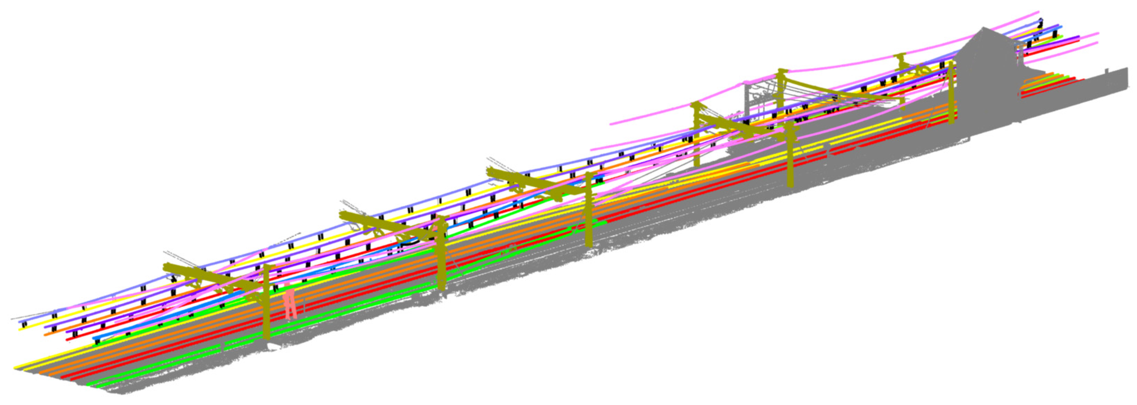
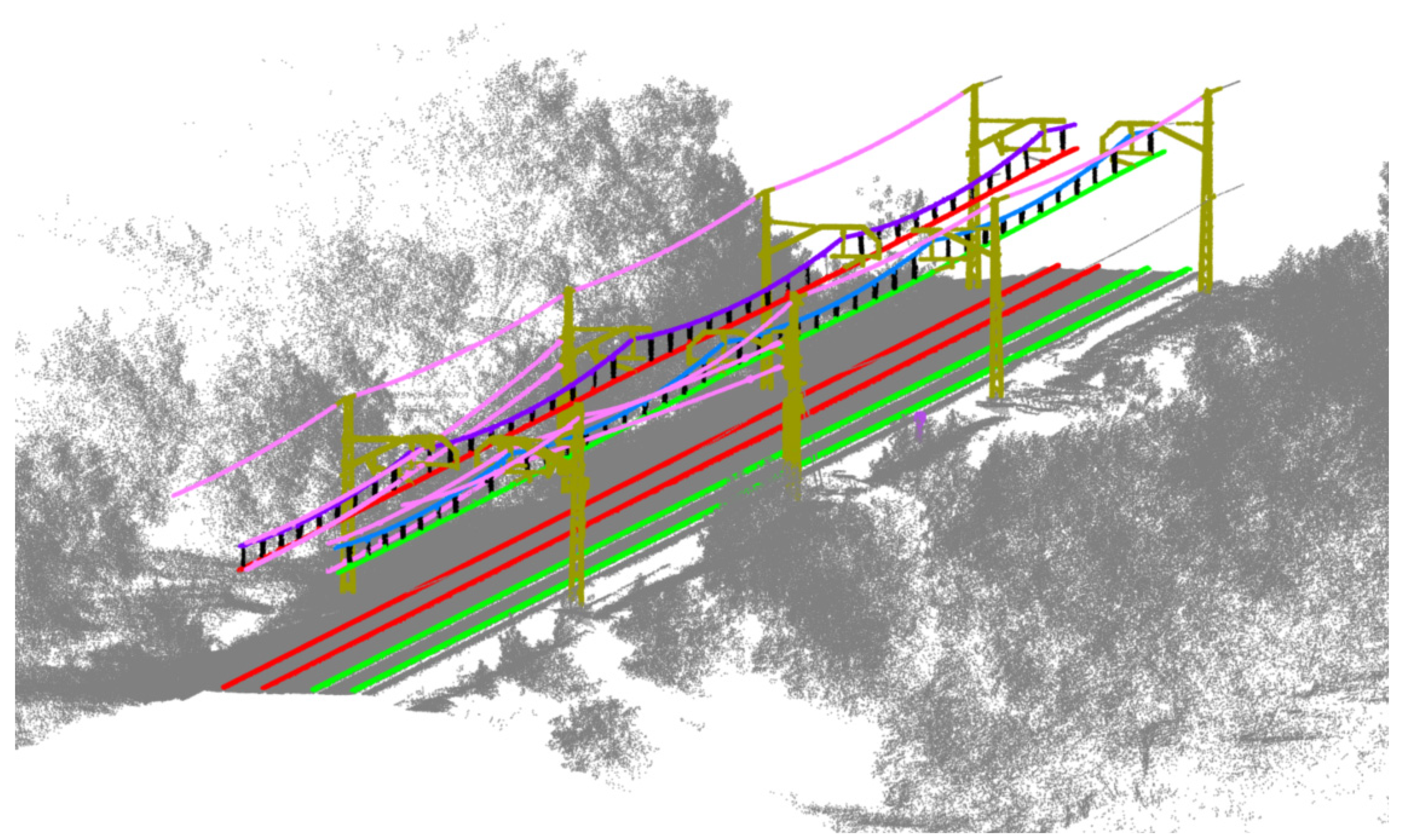
The validation process is carried out in different randomly selected C i , evaluating 9.6 km of track line, which represents 11% of the data. To evaluate the results, each selected C i is manually analysed, annotating the elements to be segmented and then comparing with the segmentation results. An example of a segmented C i is shown in Figure 15. Several segmented C i presenting different situations are shown in Appendix A.
The analysis of the elements is recorded in a confusion matrix shown in Table 3 and Table 4. It compares the manually analysed ground truth data with the segmented point cloud results. Here, point elements such as masts or signs are considered as individual objects, and continuous elements such as rails and wiring are measured in length units.
Using the results in the confusion matrix, precision, recall, and f1 score metrics are calculated for each element. They are defined in Equations (4)–(6).
p r e c i s i o n = t r u e   p o s i t i v e s t r u e   p o s i t i v e s + f a l s e   p o s i t i v e s
r e c a l l = t r u e   p o s i t i v e s t r u e   p o s i t i v e s + f a l s e   n e g a t i v e s
f 1   s c o r e = 2 p r e c i s i o n r e c a l l p r e c i s i o n + r e c a l l
In Table 3, these metrics are shown for all the segmented elements.
Finally, the processing time is also analysed and expressed in terms of second/metre. Each step of the process is also analysed, expressing its time as a percentage of the total time. (Table 5). The processing time of the different steps is summarized in Table 6.

5. Discussion

This section discusses the results of the segmentation process, highlighting the strengths and weaknesses of the described methodology.
The objective of this work is to develop a fully automated railway segmentation method able to work in several railway infrastructure scenarios in a large case study dataset, analysing the rails as well as many relevant assets of the infrastructure. The results show precision, recall, and F1 score metrics higher than 99% for rail segmentation, which is a clearly positive result, considering that the dataset has different railway lane settings, with two or three railway tracks, with railway crossings and switches. In these switches, this algorithm can segment all the rail tracks and group them, storing the information of each track separately given their correspondent contact wire, catenary wire, and droppers, which are also stored offering complete contextual information of the assets. Comparing these results with related work in [18], in which only rails are analysed, the results presented in this paper have a similar precision and a greater recall in a similar scenario with several train tracks. The results of our work are also similar to the ones obtained by [20] in a less complex scenario with only one rail track.
Results also show a good segmentation of the different wiring elements. The precision on the segmentation of contact and catenary wires is higher than 99%, and the F1 score is higher than 90%. Other wires present an F1 score higher than 85%. Comparing these results with those obtained in [21], the precision obtained is the same, but the F1 score in this study is lower. Nevertheless, as shown in the confusion matrix in Table 3, most segmentation errors appear between different wiring classes, while the approach in [21] only analyses catenary wires. The main source of error here lies in the analysis of small sections of wires that cannot be properly classified as contact or catenary and are assigned to the “other wire” class.
The other elements analysed are point elements. For these kinds of elements, the F1 score metric is also good, with results over 90% for all the elements.
In short, the results obtained in this work show the good performance of the method. Furthermore, it is important to consider the length of the dataset used in this paper, which processes 90 km of railway infrastructure data. This is considerably longer than other datasets in similar works (550 m by [20] or 2 km by [18,21]). This validates the performance of the methodology in large-scale datasets, which present more variable scenarios and dispositions of the assets for the infrastructure.

6. Conclusions

This work presents a fully automated methodology that extracts relevant assets of the railway infrastructure, such as rails, wiring and signs, traffic lights, and marks, from 3D point cloud data. First, clouds are preprocessed by sectioning them with a defined longitude and curvature, removing points far from the infrastructure, and then voxelising the selected points. Second, each section is segmented, starting with a railway track segmentation, followed by a sequential application of segmentation processes for the aforementioned elements. Finally, sections are merged and continuous elements such as rails and wires are contextually linked in the complete dataset.
The proposed method is applied to a 90 km long railway dataset. It is validated in randomly selected sections of 200 m long, covering 11% of the whole dataset in the validation process, to consider different dispositions of the railway environment. The results obtained prove the performance of the algorithm, showing an F1 score higher than 99% for rails segmentation, higher than the 90% for every other segmented element.
There are interesting future research lines from this work. First, this methodology can be followed by processes that export the required geometric and semantic information to generate infrastructure information models, following standards such as the Industry Foundation Classes (IFCs) to collect as-is models following a BIM methodology. Then, it is also interesting to analyse the segmented assets further, to check their condition, extracting parameters that can assist to the inventory of the infrastructure, or develop preventive or predictive maintenance activities. Finally, the large amount of segmented data can be used to prepare a complete and labelled dataset that can feed supervised machine learning models, saving most of the effort required for generating a manually labelled dataset and allowing faster development of artificial intelligence methods for semantic segmentation of the infrastructure.

Author Contributions

Conceptualization, M.S. and B.R..; methodology, D.L. and M.S.; software, D.L and J.G.; validation, D.L. and J.G..; investigation, M.S. and J.G.; data curation, D.L.; writing— original draft preparation, D.L. and M.S.; writing—review and editing, J.G. and B.R.; supervision B.R.; project administration, B.R.; funding acquisition, B.R. All authors have read and agreed to the published version of the manuscript.

Funding

This project has received funding from the European Union’s Horizon 2020 research and innovation programme under grant agreement No. 769255. This work has been partially supported by the Spanish Ministry of Science, Innovation and Universities through the LASTING project Ref. RTI2018-095893-B-C21. This work has been partially supported by the Spanish Ministry of Science and Innovation through the grant FJC2018-035550-I.

Institutional Review Board Statement

Not applicable.

Informed Consent Statement

Not applicable.

Conflicts of Interest

The authors declare no conflict of interest.

Glossary

C i Raw   point   cloud     i
C s k Sec tioned   point   cloud   ( k   subdivisions   of   C i )
P i   Point   i of a point cloud
T Trajectory of the mobile mapping vehicle
T C i Sec tioned   trajectory   corresponding   to   C i
T s k Sec tioned   trajectory   corresponding   to   C s k
V i Voxelised   cloud   formed   by   all   C s k   of   C i
V s k Voxelised   C s k
t s Timestamp of each point in a point cloud
I Intensity value of each point in a point cloud
V b s k Voxelised   V s k   used in ground segmentation
v 1 ,   v 2 , v 3 Eigenvectors result of applying PCA to voxel i and its neighbourhood
λ 1 ,   λ 2 , λ 3 Eigenvalues result of applying PCA to voxel i and its neighbourhood
V b t Voxels   in   V b s k   segmented as track
V t Track voxels
V p Peripherical voxels
V o Overpass voxels
V r m Mast without cantilever voxels
V m Mast voxels
V w Wire voxels
V d Dropper voxels

Appendix A

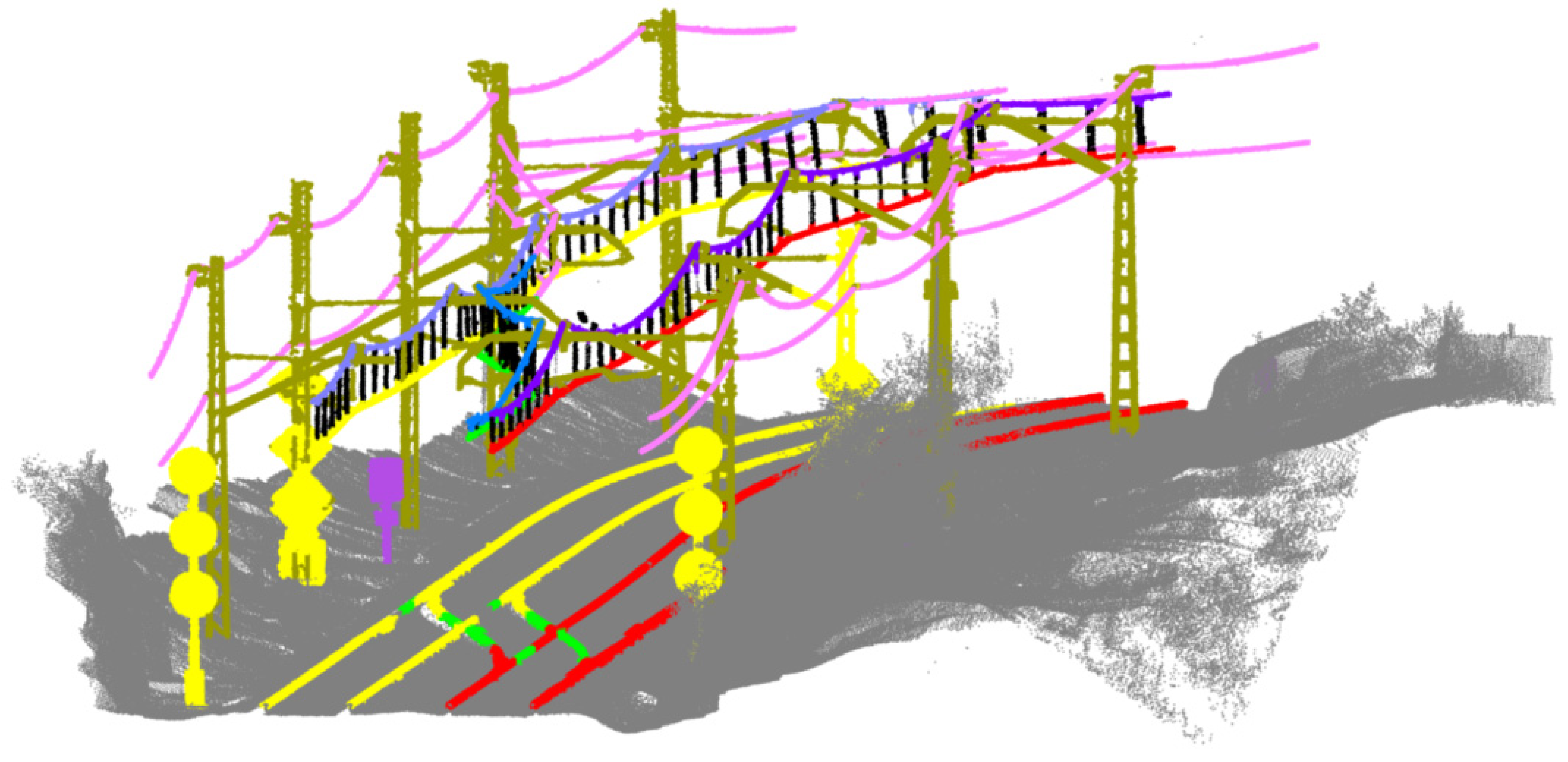
Figure A1. Railway switch: masts are represented in gold colour. Each contact wire has a different colour (yellow, green, and red), matched by its correspondent rail. Each catenary has also a random colour. Other wires are coloured in pink, droppers in black, signs in yellow, and marks in magenta.
Remotesensing 13 02332 g0a1
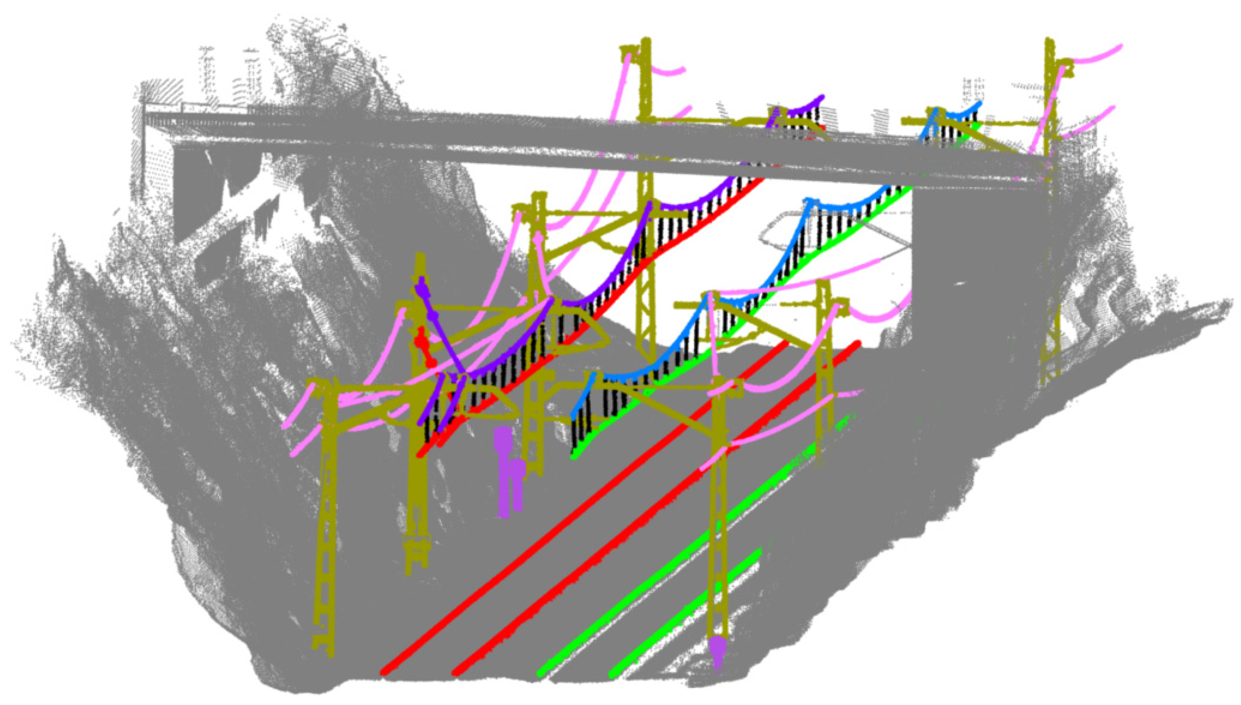
Figure A2. Railway under an overpass: masts are represented in gold colour. Each contact wire has a different colour (green and red), matched by its correspondent rail. Each catenary has also a random colour. Other wires are coloured in pink, droppers in black, and marks in magenta.
Remotesensing 13 02332 g0a2
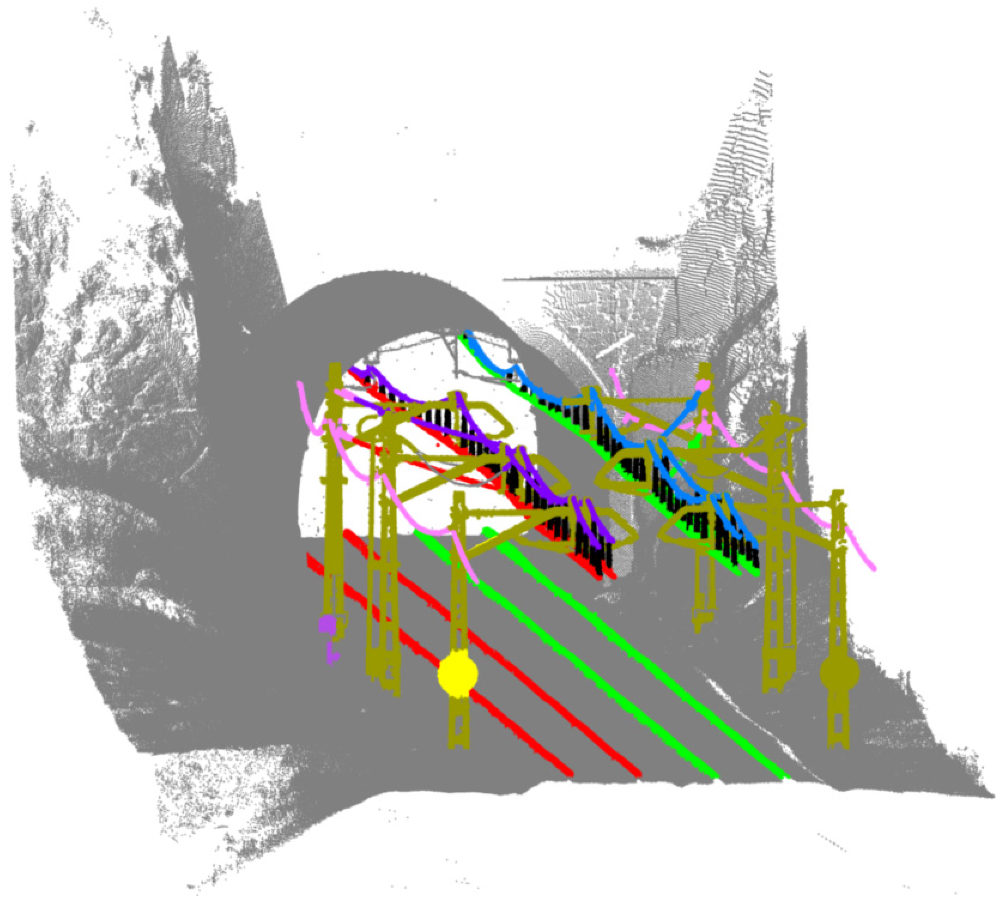
Figure A3. Tunnel entrance segmentation: masts are represented in gold colour. Each contact wire has a different colour (green and red), matched by its correspondent rail. Each catenary has also a random colour. Other wires are coloured in pink, droppers in black, and marks in magenta.
Remotesensing 13 02332 g0a3
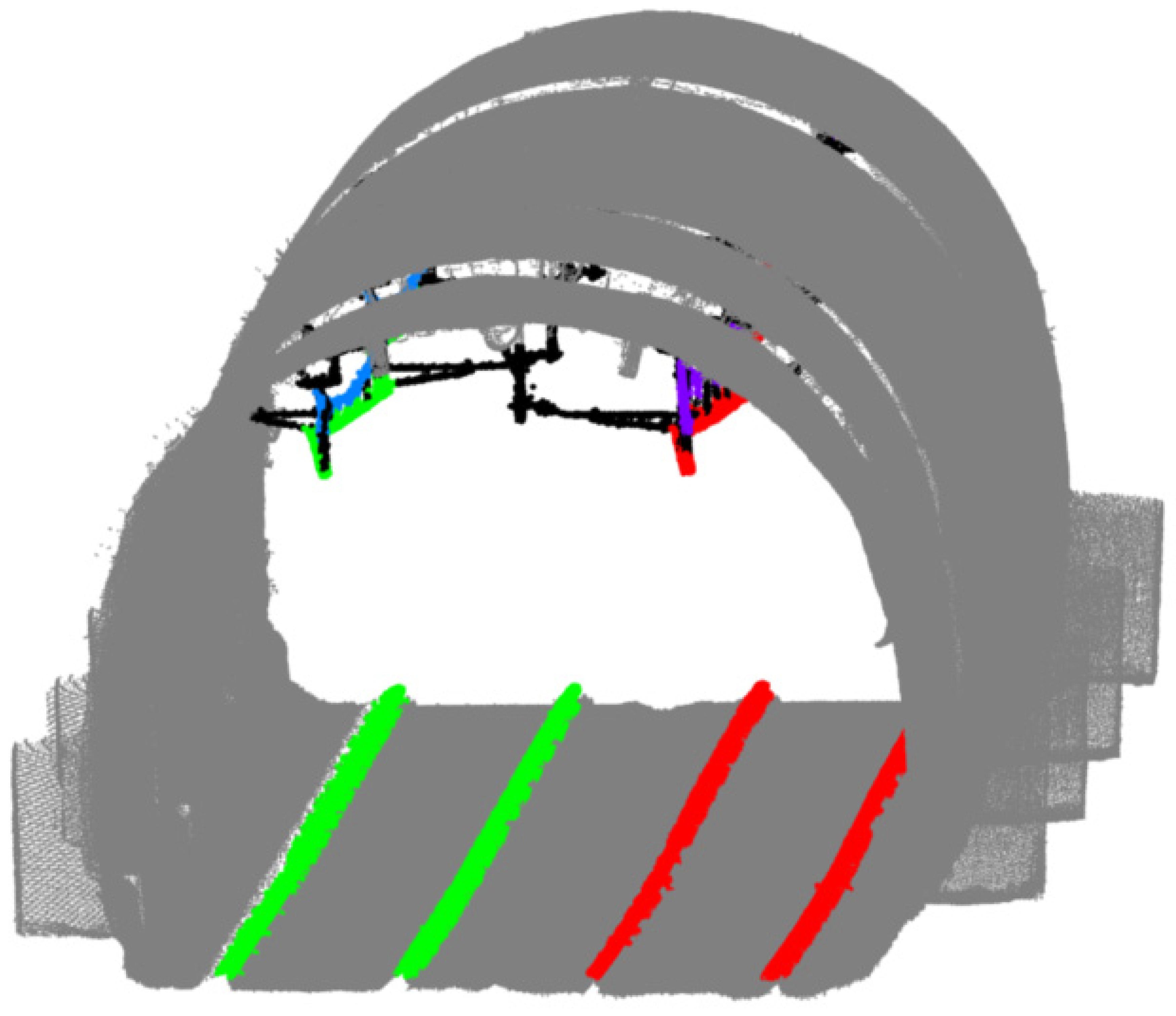
Figure A4. Railway segmentation in a tunnel: each contact wire has a different colour (green and red), matched by its correspondent rail. Each catenary has also a random colour.
Remotesensing 13 02332 g0a4
Figure A5. Four railway tracks segmentation: masts are represented in gold colour. Each contact wire has a different colour (yellow, orange, red, and green), matched by its correspondent rail. Each catenary has also a random colour. Other wires are coloured in pink, droppers in black, and traffic lights in orange.
Remotesensing 13 02332 g0a5

References

  1. Transport-Passenger transport-OECD Data. Available online: https://data.oecd.org/transport/passenger-transport.htm#indicator-chart (accessed on 26 January 2021).
  2. Statistics|Eurostat. Available online: https://ec.europa.eu/eurostat/databrowser/view/rail_ac_dnggood/default/line?lang=en (accessed on 26 January 2021).
  3. Borrmann, A.; König, M.; Koch, C.; Beetz, J. Building information modeling: Why? What? How? In Building Information Modeling: Technology Foundations and Industry Practice; Springer International Publishing: Cham, Switzerland, 2018; pp. 1–24. [Google Scholar]
  4. Isikdag, U.; Aouad, G.; Underwood, J.; Wu, S. Building Information Models: A Review on Storage and Exchange Mechanisms. Available online: https://www.researchgate.net/publication/235758990_Building_Information_Models_A_review_on_storage_and_exchange_mechanisms (accessed on 26 February 2021).
  5. Biancardo, S.A.; Intignano, M.; Viscione, N.; De Oliveira, S.G.; Tibaut, A. Procedural Modeling-Based BIM Approach for Railway Design. J. Adv. Transp. 2021, 2021, 8839362. [Google Scholar] [CrossRef]
  6. Bensalah, M.; Elouadi, A.; Mharzi, H. Integrating bim in railway projects: Review & perspectives for morocco & mena. Int. J. Recent Sci. Res. 2018, 9, 23398–23403. [Google Scholar] [CrossRef]
  7. Soilán, M.; Justo, A.; Sánchez-Rodríguez, A.; Riveiro, B. 3D Point Cloud to BIM: Semi-Automated Framework to Define IFC Alignment Entities from MLS-Acquired LiDAR Data of Highway Roads. Remote Sens. 2020, 12, 2301. [Google Scholar] [CrossRef]
  8. Cheng, Y.-J.; Qiu, W.-G.; Duan, D.-Y. Automatic creation of as-is building information model from single-track railway tunnel point clouds. Autom. Constr. 2019, 106, 102911. [Google Scholar] [CrossRef]
  9. MicroStation-Industrial Strength CAD Software for Professionals. Available online: https://www.bentley.com/en/products/product-line/modeling-and-visualization-software/microstation (accessed on 2 March 2021).
  10. Soilán, M.; Sánchez-Rodríguez, A.; Del Río-Barral, P.; Perez-Collazo, C.; Arias, P.; Riveiro, B. Review of Laser Scanning Technologies and Their Applications for Road and Railway Infrastructure Monitoring. Infrastructures 2019, 4, 58. [Google Scholar] [CrossRef] [Green Version]
  11. Ma, L.; Li, Y.; Li, J.; Wang, C.; Wang, R.; Chapman, M.A. Mobile Laser Scanned Point-Clouds for Road Object Detection and Extraction: A Review. Remote Sens. 2018, 10, 1531. [Google Scholar] [CrossRef] [Green Version]
  12. Guan, H.; Li, J.; Cao, S.; Yu, Y. Use of mobile LiDAR in road information inventory: A review. Int. J. Image Data Fusion 2016, 7, 219–242. [Google Scholar] [CrossRef]
  13. Gargoum, S.; El-Basyouny, K. Automated extraction of road features using LiDAR data: A review of LiDAR applications in transportation. In Proceedings of the 2017 4th International Conference on Transportation Information and Safety (ICTIS), Banff, AB, Canada, 8–10 August 2017; Institute of Electrical and Electronics Engineers (IEEE): Piscataway, NJ, USA, 2017; pp. 563–574. [Google Scholar]
  14. Leslar, M.; Perry, G.; McNease, K. Using mobile lidar to survey a railway line for asset inventory. In Proceedings of the ASPRS 2010 Annual Conference, San Diego, CA, USA, 26–30 April 2010; pp. 26–30. [Google Scholar]
  15. Han, Q.; Wang, S.; Fang, Y.; Wang, L.; Du, X.; Li, H.; He, Q.; Feng, Q. A Rail Fastener Tightness Detection Approach Using Multi-source Visual Sensor. Sensors 2020, 20, 1367. [Google Scholar] [CrossRef] [Green Version]
  16. Gabara, G.; Sawicki, P. A New Approach for Inspection of Selected Geometric Parameters of a Railway Track Using Image-Based Point Clouds. Sensors 2018, 18, 791. [Google Scholar] [CrossRef] [PubMed] [Green Version]
  17. Zhu, L.; Hyyppa, J. The Use of Airborne and Mobile Laser Scanning for Modeling Railway Environments in 3D. Remote Sens. 2014, 6, 3075–3100. [Google Scholar] [CrossRef] [Green Version]
  18. Yang, B.; Fang, L. Automated Extraction of 3-D Railway Tracks from Mobile Laser Scanning Point Clouds. IEEE J. Sel. Top. Appl. Earth Obs. Remote Sens. 2014, 7, 4750–4761. [Google Scholar] [CrossRef]
  19. Elberink, S.O.; Khoshelham, K. Automatic Extraction of Railroad Centerlines from Mobile Laser Scanning Data. Remote Sens. 2015, 7, 5565–5583. [Google Scholar] [CrossRef] [Green Version]
  20. Arastounia, M. Automated Recognition of Railroad Infrastructure in Rural Areas from LIDAR Data. Remote Sens. 2015, 7, 14916–14938. [Google Scholar] [CrossRef] [Green Version]
  21. Sánchez-Rodríguez, A.; Riveiro, B.; Soilán, M.; González-Desantos, L. Automated detection and decomposition of railway tunnels from Mobile Laser Scanning Datasets. Autom. Constr. 2018, 96, 171–179. [Google Scholar] [CrossRef]
  22. Soilán, M.; Nóvoa, A.; Rodríguez, A.S.; Riveiro, B.; Arias, P. Semantic segmentation of point clouds with pointnet and kpconv architectures applied to railway tunnels. ISPRS Ann. Photogramm. Remote Sens. Spat. Inf. Sci. 2020, 2, 281–288. [Google Scholar] [CrossRef]
  23. Qi, C.R.; Su, H.; Mo, K.; Guibas, L.J. PointNet: Deep Learning on Point Sets for 3D Classification and Segmentation. In Proceedings of the IEEE Conference on Computer Vision and Pattern Recognition (CVPR), Honolulu, HI, USA, 21–26 July 2017; pp. 652–660. [Google Scholar]
  24. Thomas, H.; Qi, C.R.; Deschaud, J.-E.; Marcotegui, B.; Goulette, F.; Guibas, L.J. KPConv: Flexible and De-formable Convolution for Point Clouds. In Proceedings of the IEEE/CVF International Conference on Computer Vision, Seoul, Korea, 27 October–3 November 2019; pp. 6411–6420. [Google Scholar]
  25. Soilán, M.; Nóvoa, A.; Sánchez-Rodríguez, A.; Justo, A.; Riveiro, B. Fully automated methodology for the delineation of railway lanes and the generation of IFC alignment models using 3D point cloud data. Autom. Constr. 2021, 126, 103684. [Google Scholar] [CrossRef]
  26. Home|Teledyne Optech. Available online: https://www.teledyneoptech.com/en/home/ (accessed on 3 February 2021).
  27. Soilán, M.; Riveiro, B.; Sánchez-Rodríguez, A.; Arias, P. Safety assessment on pedestrian crossing environments using MLS data. Accid. Anal. Prev. 2018, 111, 328–337. [Google Scholar] [CrossRef]
  28. Cohen-Or, D.; Kaufman, A. Fundamentals of Surface Voxelization. Graph. Model. Image Process. 1995, 57, 453–461. [Google Scholar] [CrossRef]
  29. Ester, M.; Kriegel, H.P.; Sander, J.; Xu, X. A Density-Based Algorithm for Discovering Clusters in Large Spatial Databases with Noise. In Proceedings of the 2nd International Conference on Knowledge Discovery and Data Mining KDD-96, Portland, OR, USA, 2–4 August 1996; pp. 226–231. [Google Scholar]
  30. Zhang, S.; Wang, C.; Yang, Z.; Chen, Y.; Li, J. Automatic railway power line extraction using mobile laser scanning data. Int. Arch. Photogramm. Remote Sens. Spat. Inf. Sci. 2016, XLI-B5, 615–619. [Google Scholar] [CrossRef]
  31. Silverman, B.W.; Jones, M.C.; Fix, E. An Important Contribution to Nonparametric Discriminant Analysis and Density Estimation: Commentary on Fix and Hodges (1951). Int. Stat. Rev. 1989, 57, 233–238. [Google Scholar] [CrossRef]
  32. Sánchez-Rodríguez, A.; Soilán, M.; Cabaleiro, M.; Arias, P. Automated Inspection of Railway Tunnels’ Power Line Using LiDAR Point Clouds. Remote Sens. 2019, 11, 2567. [Google Scholar] [CrossRef] [Green Version]
  33. Arastounia, M.; Elberink, S.O. Application of Template Matching for Improving Classification of Urban Railroad Point Clouds. Sensors 2016, 16, 2112. [Google Scholar] [CrossRef] [PubMed] [Green Version]
Figure 1. Casa study data. 90 km of railway section.
Remotesensing 13 02332 g001
Figure 2. Proposed methodology workflow.
Remotesensing 13 02332 g002
Figure 3. Sectioning workflow: (a) point cloud C i with its corresponding trajectory section T C i ; (b) C i is sectioned in C s k and C s ( k + 1 ) with its corresponding T s k and T s ( k + 1 ) . C i points that are not part of any section are coloured in grey.
Remotesensing 13 02332 g003
Figure 4. MPCA: X 0 ,   Y 0 ,   Z 0 are the world coordinates; X p c a ,   Y p c a ,   Z p c a , are the PCA eigenvectors applied in A; X m p c a ,   Y m p c a ,   Z m p c a are the MPCA eigenvectors applied in A.
Remotesensing 13 02332 g004
Figure 5. Voxel’s neighbours numbering. The numeration is organised by levels in the Z dimension.
Remotesensing 13 02332 g005
Figure 6. Track segmentation: green voxels are segmented as track; red voxels are segmented as peripherical voxels; dark voxels are segmented as overpass.
Remotesensing 13 02332 g006
Figure 7. Masts’ segmentation workflow: (a) voxels with vertical neighbourhood distribution; (b) clusters which meet the “Mast without cantilever” model specifications; (c) previous clusters, coloured in red, and the new voxels added to each mast, coloured in green; (d) possible cantilever’s voxels, i.e., voxels whose neighbourhood has no dispersion in the trajectory direction; (e) masts without cantilever, coloured in red, and cantilevers, coloured in green.
Remotesensing 13 02332 g007
Figure 8. Wiring segmentation workflow: (a) voxels whose neighbourhood has a linear distribution in the trajectory direction; (b) clustered voxels, each cluster as a different colour; (c) remaining clusters once they are filtered by longitude, linearity, and density; (d) classified clusters. Contact wires are coloured in green, catenary wires in red, and other wires in yellow.
Remotesensing 13 02332 g008
Figure 9. Droppers’ segmentation workflow: (a) bounding box of contact–catenary wires; (b) voxels inside the bounding box unclassified coloured in black and their neighbours in red; (c) droppers coloured in red, catenary wires in yellow, and contact wires in green.
Remotesensing 13 02332 g009
Figure 10. Signage elements’ segmentation workflow: (a) voxels of possible signage elements coloured in black; (b) clustered voxels, each cluster as a different colour; (c) signage elements, each type of element as a different colour.
Remotesensing 13 02332 g010
Figure 11. Signage elements classification process: (a) checking the orientation; (b) checking the form; (c) checking its dimensions; (d) checking the distance to the point cloud of the model.
Remotesensing 13 02332 g011
Figure 12. Signs on masts segmentation: (a) intensity normalised histogram of voxels in a mast; (b) signs on masts segmented as with an intensity higher than the first local minimum (red colour) and their neighbours (yellow colour).
Remotesensing 13 02332 g012
Figure 13. Rail segmentation workflow: (a) contact wire coloured in green corresponding to the rails under study; (b) rails and its surrender. Left rail coloured in yellow and right rail in red; (c) rail filtered by height. Rough rails coloured in green, left rail coloured in yellow, and right rail in red; (d) rails filtered by the distance between them. Starting rails coloured in green, left rail coloured in yellow, and right rail in red; (e) rails refined in C i . Starting rails coloured in green, left rail coloured in yellow, and right rail in red.
Remotesensing 13 02332 g013
Figure 14. Output data structure: track n is the structure with the elements of the track number n in a C i , formed by its rails, contact, catenary, and droppers. Element type X is a structure with all the elements in C i of a certain class, namely, signs, traffic lights, marks, masts, or signs in masts.
Remotesensing 13 02332 g014
Figure 15. Results of the segmentation method: masts are represented in gold colour. Each contact wire has a different colour, matched by its correspondent rail. Each catenary has also a random colour. Other wires are coloured in pink, droppers in black, and marks in magenta.
Remotesensing 13 02332 g015
Table 1. Models used in the segmentation process to define the parameters of the algorithms and to analyse clusters of points comparing them with the specifications of each model. The dimensions of the models are defined in X ,   Y ,   Z . Their shapes are defined by the eigenvalues obtained applying PCA. Their orientation is defined by the eigenvectors obtained applying PCA, represented in a 3 × 3 matrix, being sorted by columns. The deviation to those eigenvectors is defined in degrees. The template is a set of points formed by the points of a given element manually extracted from the data and the distance to that template is calculated with Equation (3).
Models Dimensions   X ,   Y ,   Z   [ m ] Shape
(Eigenvalues PCA)
Orientation
(Eigenvectors PCA)
Tolerance Orientation [Degrees]Template Tolerance   Distances   to   the   Template   [   m 2 ]
S i g n 0.34 ± 0.14 1.1 ± 0.3 5 ± 1 0.96 ± 0.03 0.03 ± 0.02 0.01 ± 0.01 0 0 1 0 1 0 1 0 0 7 10 10 No-
T r a f f i c   l i g h t 2 ± 1 0.65 ± 0.2 0.92 ± 0.05 0.07 ± 0.05 0.01 ± 0.05 0 0 1 15 Yes
(3 templates)
0.03
M a r k 0.25 ± 0.1 0.35 ± 0.1 0 0 1 0 1 0 1 0 0 15 25 25 Yes
(2 templates)
0.001
M a s t   w i t h o u t   c a n t i l e v e r 1.2 ± 1.2 0.75 ± 0.75 10 ± 4 0.85 ± 0.15 0 0 1 20 No-
W i r e 0.3 No-
D r o p p e r 1 ± 1 No-
R a i l 0.3 No-
P a i r   o f   r a i l s 0.74 No-
Table 2. Values of the parameters involved in the methodology.
ProcessParameterValueParameterValue
General g v 0.1 mElementsTable 2
d 1 0.3     g v m d 1 0.6     g v m
Sectioning l s 100 m c u r s 5 m
w s 20 m o v s 5 m
Track
segmentation
r m t 0.5 m g v B 0.3 m
s t t 3     g v m p t 3 / g v B voxels/cluster
c l t 1.3     g v m p r 100 / g v voxels/cluster
e v t r 0.7
Masts
segmentation
m z 0.7 m x 0.5
m y 0.5 m c x 0.5
c l m 1.5     g v m p e r w 50%
Wiring
segmentation
w z 0.5 l w 9 m
w l a t 0.7 w d 0.7 / g v voxel/m
s t w 0.2 m d i s t w 4 m
m s w 0.1 m
Droppers
segmentation
c l t 0.2     g v m p s 100 / g v voxels/cluster
Signs on masts
segmentation
p s i g 2% c l s 1.3     g v m
h s 20 p r 2 / g v voxels/cluster
Rails segmentation m s r 0.75 m s t r 0.5
b r 0.02 m
Merging m s x 10 m m s y 2 m
Table 3. Confusion matrix of continuous elements measured in metres.
PredictedRail [m]Contact [m]Catenary [m]Other Wire [m]No Class [m]
Real
Rail [m]3747400090
Contact [m]02134802900134
Catenary [m]00211983050134
Other wire [m]0100100249291838
No class [m]6005-
Table 4. Confusion matrix of point elements measured in number of elements.
PredictedDropperMastTraffic LightSignMarkSign MastNo Class
Real
Dropper559700000910
Mast043500009
Traffic Light00140001
Sign00015002
Mark00005903
Sign mast00000234
No class850001-
Table 5. Precision, recall, and F1 score.
ElementPrecisionRecallF1 Score
Rail99.98%99.76%99.87%
Contact99.53%87.56%93.16%
Catenary99.53%86.94%92.81%
Other wires80.72%92.44%86.18%
Dropper99.86%86.02%92.42%
Masts98.86%97.97%98.42%
Traffic light100.00%93.33%96.55%
Sign100.00%88.24%93.75%
Mark100.00%95.16%97.52%
Sign in mast95.83%85.19%90.20%
Table 6. Processing time.
ProcessTime
Total process1.96 s/m
Loading point cloud1.71%
Sectioning1.14%
Voxelised6.36%
Segmentation90.79%
Selecting section1.88%
Track4.01%
Local PCA11.88%
Masts41.17%
Wiring7.69%
Droppers0.57%
Signs6.51%
Rails16.68%
Merging sections0.05%
Indexes   from   V i   to   C i 0.35%
Publisher’s Note: MDPI stays neutral with regard to jurisdictional claims in published maps and institutional affiliations.