Abstract
Vegetation phenology plays a key role in influencing ecosystem processes and biosphere-atmosphere feedbacks. Digital cameras such as PhenoCam that monitor vegetation canopies in near real-time provide continuous images that record phenological and environmental changes. There is a need to develop methods for automated and effective detection of vegetation dynamics from PhenoCam images. Here we developed a method to predict leaf phenology of deciduous broadleaf forests from individual PhenoCam images using deep learning approaches. We tested four convolutional neural network regression (CNNR) networks on their ability to predict vegetation growing dates based on PhenoCam images at 56 sites in North America. In the one-site experiment, the predicted phenology dated to after the leaf-out events agree well with the observed data, with a coefficient of determination (R2) of nearly 0.999, a root mean square error (RMSE) of up to 3.7 days, and a mean absolute error (MAE) of up to 2.1 days. The method developed achieved lower accuracies in the all-site experiment than in the one-site experiment, and the achieved R2 was 0.843, RMSE was 25.2 days, and MAE was 9.3 days in the all-site experiment. The model accuracy increased when the deep networks used the region of interest images rather than the entire images as inputs. Compared to the existing methods that rely on time series of PhenoCam images for studying leaf phenology, we found that the deep learning method is a feasible solution to identify leaf phenology of deciduous broadleaf forests from individual PhenoCam images.
1. Introduction
Vegetation phenology denotes periodic phenomena affected by climate, hydrology, soil, and other environmental conditions, which accompanies key events such as germination, leaf expansion, flowering, leaf discoloration, and defoliation [1,2]. Changes in leaves reflect the high sensitivity of vegetation to seasonal weather and climate variability [3,4,5]. Leaf phenology alters physical characteristics of the land surface such as albedo and roughness [6], which also influences the biogeochemical processes such as photosynthesis and transpiration [7,8]. Monitoring leaf phenology is important for us to understand the interactive relationship between a changing climate and terrestrial ecosystems.
Available approaches to collect phenological data include field measurements, near-surface observations, and airborne and space-borne remote sensing. Field measurements date back over 2000 years [9] and still play a role today in recording phenology changes of individual trees such as flowering or budburst [10,11]. Field measurements of leaf phenology involve extensive fieldwork, making it difficult to conduct long-term and high-frequency experiments. Airborne and space-borne remote sensing is able to provide repetitive and synoptic land surface observations and offers opportunities to monitor vegetation phenology on a small scale across large areas [12]. The use of satellite data has promoted macro-scale phenology studies under the context of global climate change [13,14]. Remote sensing observations however often have quality issues such as sensor degradation and cloud contamination and are affected by platform revisit periods and sensor resolutions. The inversion algorithms including underlying assumptions and parameter settings also contribute uncertainties in retrieved phenology metrics from time series of remote sensing data [15]. Near-surface observation from eddy covariation flux towers has been used to derive and study leaf phenology changes. Eddy covariation flux towers that continuously monitor vegetation canopies could provide observations of land-atmosphere fluxes on an hourly or half-hourly basis. Because phenological events typically occur only once or twice a year, the phenological metrics retrieved from eddy covariation flux towers are limited by the availability of the tower sites [16].
In recent years, digital photography has provided an automated and cost-effective approach to monitoring leaf dynamics at the canopy level [17]. The method called PhenoCam involves mounting digital cameras with visible-wavelength imaging sensors above vegetation canopies to capture images throughout the day [18]. Near-surface observations from PhenoCam provide time series of images that are ideal for tracking seasonal changes in leaf phenology [19]. As high-quality and low-cost digital cameras are now widely available, PhenoCam has been increasingly deployed for ecological studies. PhenoCam images have been used to extract leaf phenology metrics [20] and track biodiversity [21]. Zhang et al. monitored vegetation growth over time using both PhenoCam and remote sensing data [14]. Wang et al. estimated vegetation gross primary productivity on a daily bias using PhenoCam data to reduce modelling uncertainties [22]. Wu et al. studied the relationship between leaf ages and canopy characteristics using PhenoCam data [23]. The current studies have proven that PhenoCam images carry useful information for monitoring and understanding leaf phenology.
To date, most studies use indirect methods to identify phenology variation based on the time series of PhenoCam images. The indirect methods track changes in images by deriving handcrafted features such as green chromatic coordinate (GCC) [24,25] and red chromatic coordinates (RCC) [1] from PhenoCam images and then apply algorithms to derive the timing of phenological events, such as start-of-growing season (SOS) and end-of-growing season (EOS). The use of handcrafted features such as GCC or RCC overlooked high-level information in digital images. More importantly, these studies generally required at least two images or even the time series to obtain information related to leaf phenology. In this study, we aim to propose a method that can predict the daily leaf growth time with the provided PhenoCam image only. Specifically, leaf growth time refers to the period between SOS and EOS, and we predict the day of that period for individual PhenoCam images.
Deep learning, as a subset of machine learning, is able to automatically learn the relationships between features and tasks. The way to extract complex features from input data in deep learning is different from traditional shallow learning. Deep learning transforms the features of the sample in the original space to a new feature. Deep learning methods have been widely used for image processing in the fields such as computer vision, speech recognition, and natural language processing [26]. In remote sensing, deep learning approaches have been used to process the tasks of image classification, segmentation, and object recognition. Compared with traditional classification methods, the deep learning model often provides higher processing accuracy when large samples for model training and testing are available. The image data recorded by PhenoCam has been accumulated in recent years, and it is of interest to further explore the recorded dataset. The development of deep learning approaches provides the possibility to process and make predictions on individual images. Recent studies on facial age recognition and image segmentation using the deep learning models inspire us to test identification of leaf phenology from PhenoCam images.
The main goal of this study was to identify the leaf phenology of deciduous broadleaf forests from individual PhenoCam images using deep learning methods. In other words, we tested the deep learning models on predicting leaf growing dates after SOS in a year from a given PhenoCam image. Compared with traditional methods that predict leaf phenology with handcrafted features from time series data, the use of deep learning methods allows us to infer daily leaf phenology from individual PhenoCam images and can potentially improve image processing accuracy and reduce labor costs.
2. Study Materials
The PhenoCam network, established in 2008, initially provided automated monitoring of leaf phenology in forest ecosystems in the northeastern United States and neighbouring Canada [27], and later expanded to give long-term observations covering a variety of geographic sites. More than 600 site cameras in the PhenoCam network are now deployed across a wide range of ecological, climatic, and plant functional types in North America. Most sites upload one digital photo every 30 min from 04:00 am to 9:30 pm local time. These photos are stored on servers at the University of New Hampshire [28]. The archived dataset currently has approximately 15 million images requiring 6 TB of disk space and provides a record that can be used to determine the phenological state of leaves [27]. High-quality data is ensured by minimizing data discontinuity due to adverse weather conditions (e.g., rain, snow, and hail), adverse light conditions (e.g., cloud and aerosol), or short-term power outages [29]. The PhenoCam dataset is publicly available on the website of the PhenoCam project (http://phenocam.sr.unh.edu/; accessed on 18 September 2020).
In the PhenoCam dataset, there are three types of observation sites, namely Type I, II, and III sites. The Type I sites follow a standard protocol to ensure data quality and data continuity [27], whereas the Type II and III sites are required to obey the standard protocol. The key aspects of the standard protocol are as follows. Firstly, the camera is set to fix the white balance. Secondly, the camera is mounted at a safe point and tilted down at 20–40 degrees such that its field of view covers the landscape. Ideally, the acquired image mainly consists of vegetation and a small part of the sky. Thirdly, in the northern hemisphere, the camera is pointed to the north to reduce the lens flares, shadows, and forward scattering of the canopy. Basic information for each PhenoCam site, including site category, site location, the start and end dates of site images, the camera model, vegetation type, the climate, and site attributes, is included in the data record.
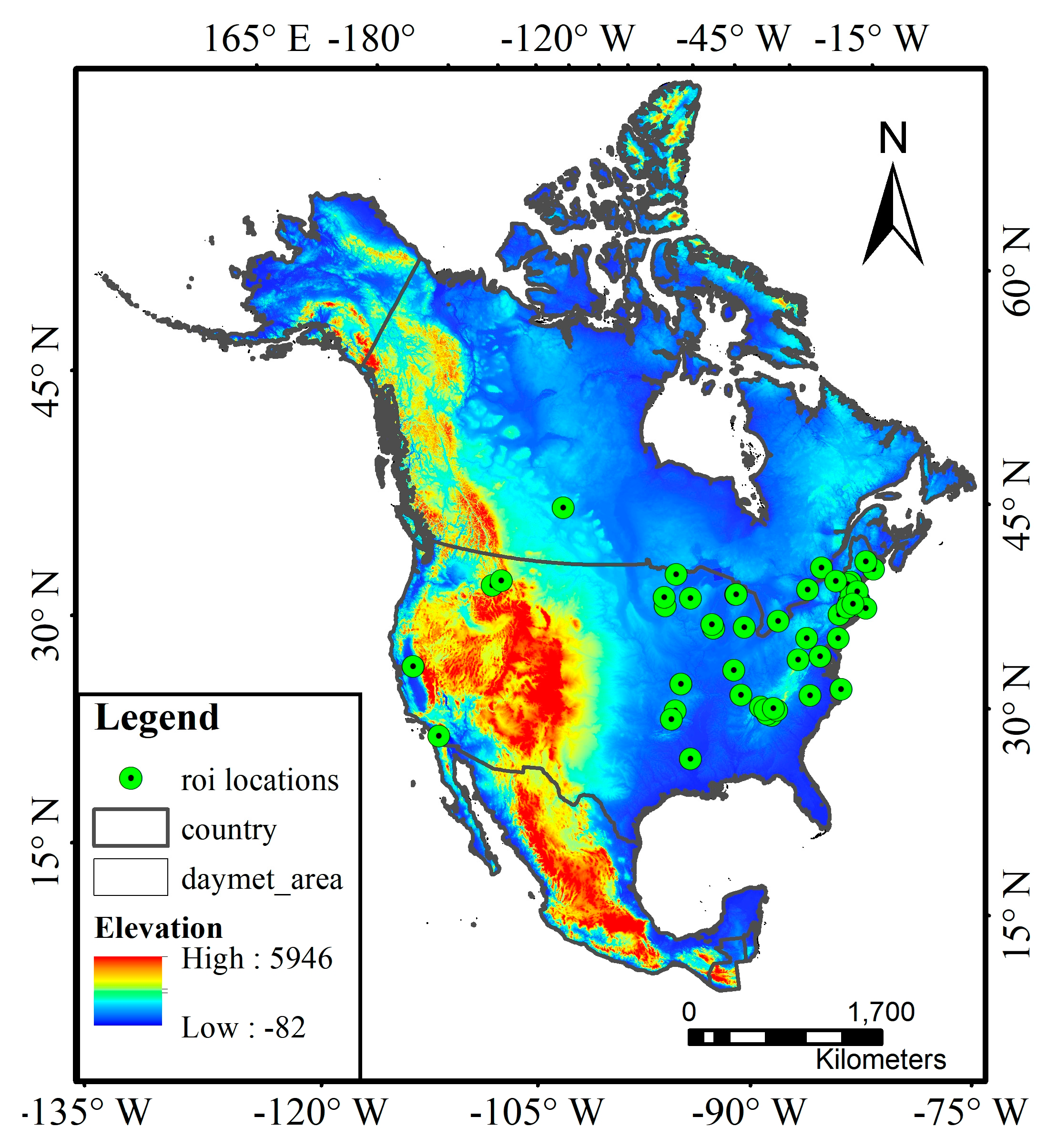
We used the data from 56 deciduous broadleaf forest sites in North America in the PhenoCam 1.0 version dataset. Figure 1 shows the spatial distribution of the studied PhenoCam sites, which are mainly distributed across the latitude range of 32°–47°N with an elevation up to 1550 m. Most sites are situated in the temperate continental climate zone. We chose the Type I sites of deciduous broadleaf forests that follow the standard protocol. We used the images that were taken within 11:30 am–1:30 pm local time every day, given that images acquired in the early morning and late afternoon were often affected by sunlight scattering.
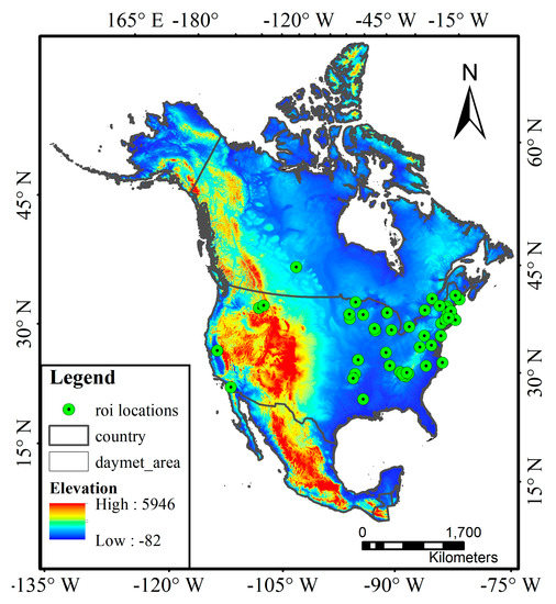
Figure 1.
The spatial distribution of the studied PhenoCam sites in North America overlaid on the elevation map, with the map reference system of WGS84. The detailed sample information of each site is shown in Table A1.
3. Methods
Our goal was to predict the leaf growing days of deciduous broadleaf forests in a growing season (from SOS to EOS) from each PhenoCam image using deep learning models. We determined the dates of leaf-out based on the time series of GCC and labelled the dates after leaf-out for each image. As our task was to solve a regression problem rather than a classification problem, we modified the CNN-based models to fit in the regression task. We trained and evaluated four different CNN-based models at three different temporal scales.
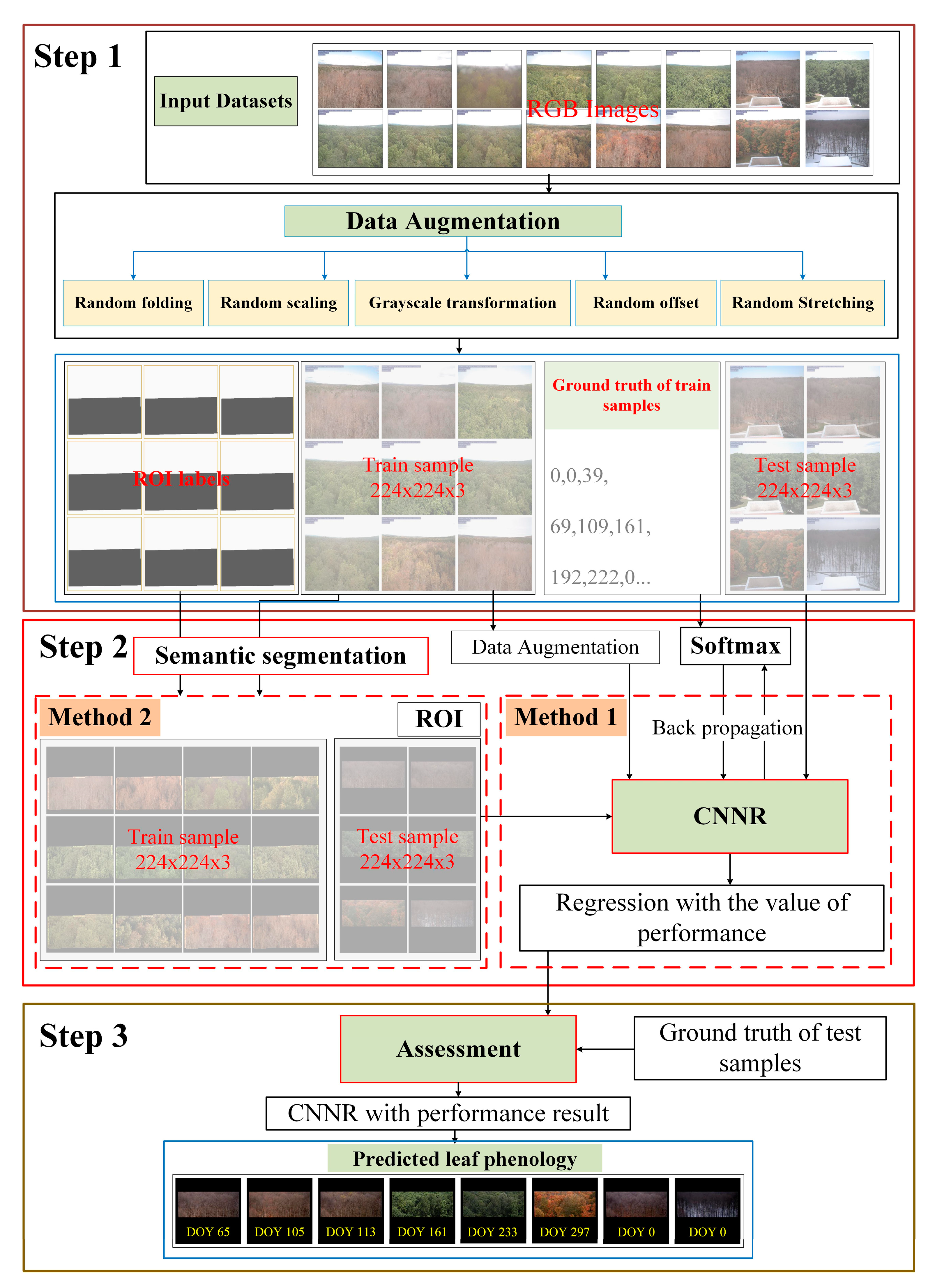
The architecture shown in Figure 2 illustrates the workflow of our study and it includes three main parts. The first part is data preprocessing, including data labelling and augmentation. The second part is the leaf phenology prediction based on deep learning methods, in which two strategies were used. For the first strategy, we used CNNRs to predict leaf phenology from PhenoCam images directly; in other words, we fed the entire PhenoCam image into the CNNRs. For the second strategy, to investigate whether background information in the PhenoCam images such as the sky or other land covers influences the accuracy of leaf phenology, we used semantic segmentation models to identify region-of-interests (ROIs) in the Phenocam images first and then fed the ROI images into the CNNRs. ROIs denote a subset in the Phenocam images and only includes vegetation canopies and excludes backgrounds. ROIs in the Phenocam dataset has already been manually labelled by camera maintainers and can be downloaded directly from the official website. As ROIs were labelled for only a few sites, we employed a semantic segmentation method based on deep learning to detect ROIs from the PhenoCam images for all sites. The last part is the leaf phenology evaluation. The detailed methodology is introduced in the following sections.
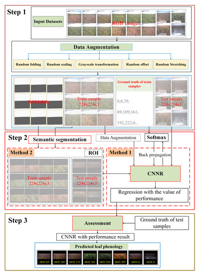
Figure 2.
The flowchart for leaf phenology prediction is based on the CNNRs. Step 1 shows the preprocessing of the raw input data, including data augmentation and transformation; Step 2 displays the deep learning processing, including direct CNNRs (method 1) and regression after ROIs detection (method 2); and Step 3 demonstrates the model assessment.
3.1. Data Preprocessing
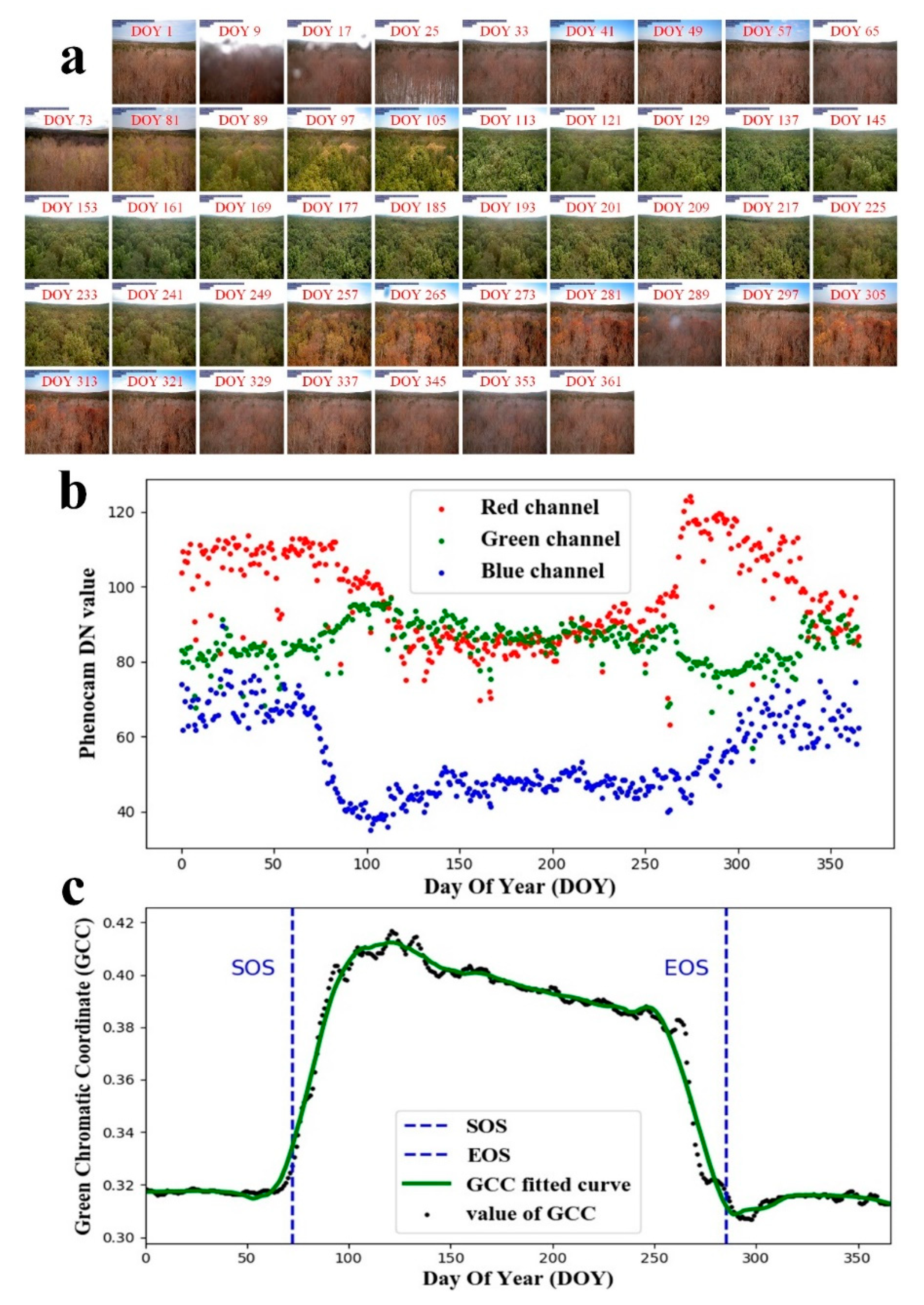
To feed the PhenoCam images into the CCNRs for training and testing, we needed to do a series of data processing. Data preprocessing mainly included two steps, i.e., training and testing image data selection and image labelling. As the PhenoCam images are often influenced by animals and climate (Figure A1), we needed to choose available data set for the experiment. In this study, we selected images that had no animal tracks and no climate contaminations, such as rainfall, fog, and solar flare. In total, 14,453 PhenoCam images from 56 sites were chosen for study, which was downloaded from the PhenoCam website (https://phenocam.sr.unh.edu/webcam/tools/; accessed on 18 September 2020). Figure 3. (a) illustrates phenology changes of the PhenoCam images at a deciduous broadleaf forest. We only show the PhenoCam images every eight days as examples, although there are PhenoCam images every day. The PhenoCam images generally consist of three visible bands including red, green, and blue bands, and occasionally contain the near-infrared band at a few sites. The image sizes of the raw data and the label data are not the same across the sites, ranging from 640 × 480 pixels at the Bartlett site to 4000 × 2500 pixels at the Coville site. We cropped the images to the same size of 224 × 224 pixels.

Figure 3.
Leaf changes at the site of Dukehw Station are shown for (a) every 8-day PhenoCam images across one year, (b) averaged digital numbers (DN) in the red, green, blue bands, respectively, at every 30-min intervals, and (c) the fitting curve of GCC across one year, the black dot represents the GCC value derived from individual image, and the green curve denotes the fitting line of the GCC time series. DOY denotes the day of the year. SOS and EOS denote the start of the season and the end of the season, respectively.
In the image labelling process, we defined leaf growing dates sequentially from the start of season (SOS) to the end of season (EOS) daily. Both SOS and EOS are defined based on the fitted GCC curve (Figure 4c). The SOS is defined as the date when GCC first reaches 10% of the seasonal amplitudes in the rising stage (the blue vertical dotted line on the left in Figure 4c), and EOS is defined as the date when GCC first exceeds 90% of the seasonal amplitudes in the declining stage (the blue vertical dotted line on the right in Figure 4c). SOS is the first day of leaf growth in a year, and EOS is the last day of leaf growth in a year. We labelled leaf growing date for each PhenoCam image between SOS and EOS as the date starting from SOS, and labelled leaf growing dates for the images before SOS or after EOS in a year as 0 because leaf growth is in a dormancy stage. The dates associated with major changes in leaf colour characteristics, such as greenness rise, and greenness decline, were derived from high-frequency images collected over the past ten years on daily scales [27]. The acquisition frequency of the PhenoCam data is important for studying temporal changes in leaf colour characteristics. There is a complete image data file processed for each phenology site, namely the summary product, which contains the calculation results of daily GCC time series. We used the daily product and eliminated outliers as we aim to predict leaf phenology from each image on a daily scale. Moreover, we investigated the proposed leaf phenology prediction method at different time scales and selected 8-day and 80-day data for additional experiments. In the additional experiments, the date of leaf growth is divided into few sessions, for example, day 1–8, day 9–16, and so on in the 8-day experiment.
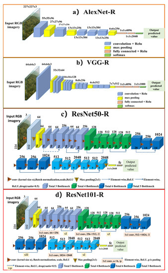
Figure 4.
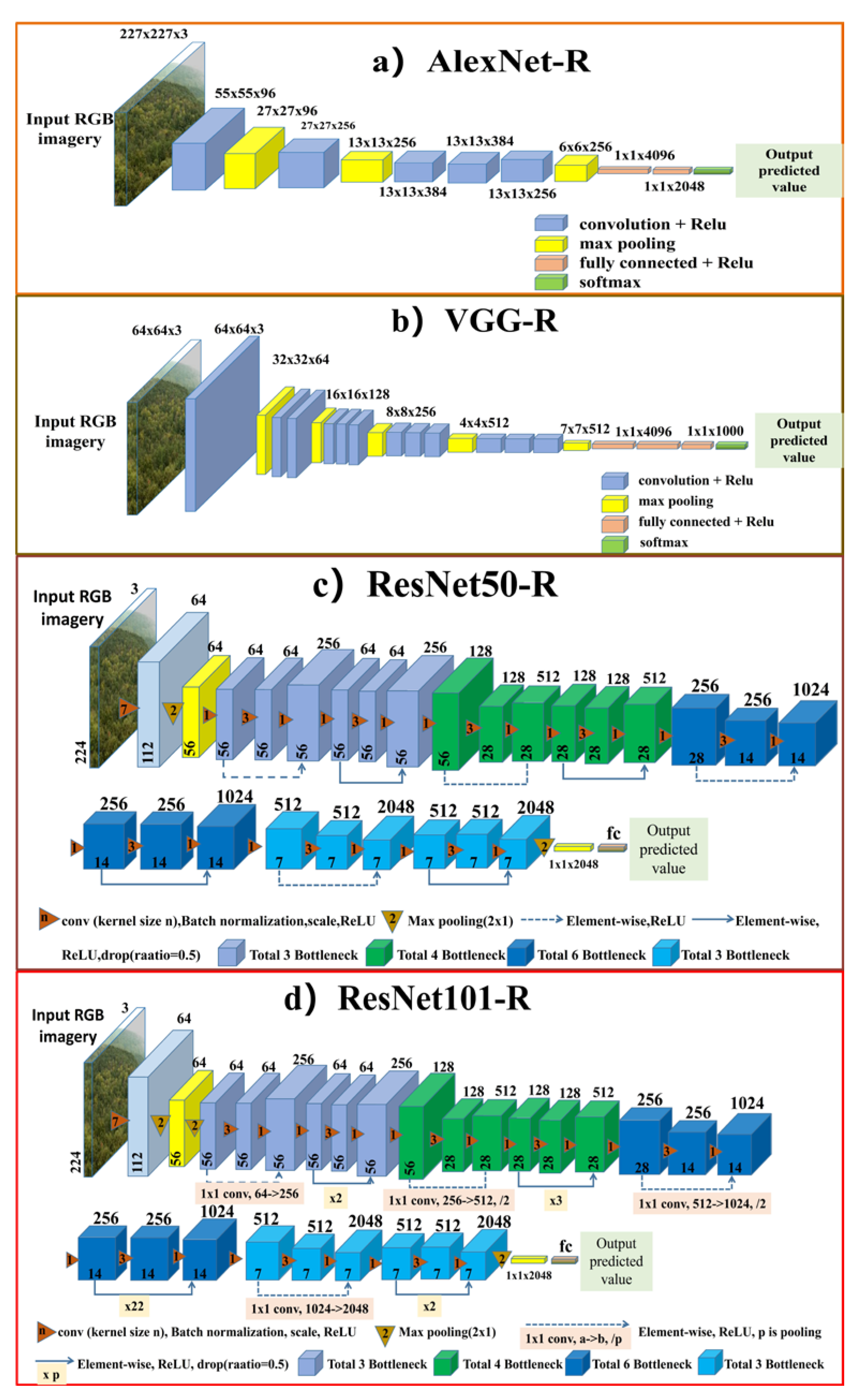
The architectures of four CNNRs used in leaf phenology prediction. The CNNRs are adapted and modified from AlexNet [30], VGG [31], ResNet50, and ResNet101 [33]. The numbers on the top of each box denote the band number of the feature maps, and the numbers on the bottom of each box denote the height and width of the feature maps. Figure 4. (a) represents the architecture of AlexNet-R, (b) represents the VGG-R structure, (c,d) represent the ResNet50-R and ResNet101-R, respectively.
For each selected PhenoCam image, we determined its leaf growing date using GCC. Owing to noise originating from factors such as weather, sun illumination geometry, and exposure controls, the original PhenoCam images were rarely used directly in past phenology studies. Methods have been developed to convert the digital numbers of each pixel to chromatic indices such as GCC and RCC. Studies have found that the time series of GCC or RCC is representative of the seasonal trajectory of leaf growth and activities [17]. The calculation method of GCC in the summary product we used is as follows (Equation (1)):
where, , , and denote the digital numbers in red, green, and blue bands, respectively.
We conducted the quality control processes such as filtering and outlier detection for the GCC time series and inspected the processed time series of GCC visually. Missing data in the GCC time series were linearly interpolated based on nearest neighbor points. In this part, the least square method and the Savitzky-Golay smoothing algorithm were employed for the fit of the interannual GCC curve. The hyperparameters used for the Savitzky-Golay smoothing algorithm were as follows: the window size was set as 53 and the polynomial order was 3. Figure 3. (c) shows both the derived GCC time series and its fitted curve corresponding to the growing cycle of leaves.
3.2. Leaf Phenology Prediction
In the first strategy, four modified convolutional neural network regression methods (CNNRs, Figure 4) were used to predict the leaf growing dates for deciduous broadleaf forests. The used CNNRs were derived from the commonly used convolutional neural network (CNN) structures. The CNN models have been proven advantageous over traditional machine learning methods in extracting low-level and high-level features from images. Accompanying with the development of hardware and public datasets, researchers have proposed various CNN models to improve image classification, among which the widely used ones include AlexNet [30], Visual Geometry Group (VggNet) [31], GoogleNet [32], and Deep Residual Network (ResNet) [33]. Here we use the four networks, i.e., AlexNet, VGG, ResNet50, and ResNet101, as the backbones for predicting leaf phenology from individual PhenoCam images. The architectures of four used CNNRs are shown in Figure 3. AlexNet is an 8-layer deep CNN, which can solve over-fitting problems through multiple skills such as dropout and Relu. VGG is an improvement of AlexNet. It uses a smaller convolution kernel and stride in the first convolution layer, which is suitable for multi-scale training and testing. Compared to both AlexNet and VGG, ResNet overcomes the problem of gradient explosion and disappearance [34]. The residual module in ResNet enables the gradient transmission and low-level information retaining through a linear connected path. In our leaf phenology prediction task, we inherit the convolution layer and the pooling layer of each network, but use a regression loss function rather than the cross-entropy loss function for regression analysis. For ResNet, we tested two different depth structures, which are 50-layer (ResNet50) and 101-layer (ResNet101). Finally, AlexNet-R, VGG-R, ResNet50-R and ResNet101-R are used for leaf phenology prediction. We used MSELoss for optimizing the task of phenology prediction. The MSELoss function is suitable for the regression problems, which expresses averaged sum of the squares of the difference between the predicted values and ground truth.
3.3. Leaf Phenology Prediction Using Detected ROI Images
As mentioned above, we adopted the second strategy to predict leaf growing dates based on ROIs detected from each PhenoCam image. Compared with the first strategy, there is a need to extract representative ROIs from PhenoCam images first. ROIs contain only canopies compared to the entire PhenoCam image that includes background information such as the sky, buildings, lakes, and animals. ROIs masked out the background and the use of ROIs possibly reduces the influence of background factors on the prediction accuracies.
Semantic segmentation is a process that separates the regions of different objects and labels their categories for a given image [35]. Currently, there are various semantic segmentation networks available to label each pixel in an image, such as FPN [36], Unet [37], DeeplabV3+ [38], and PSPNet [39]. These networks often have encoder-decoder architectures, and used various up-sampling structures in the decoder part to restore the compressed features generated from the encoder part to the same size as the input image. In our previous work, we proposed BAPANet [40], which is a robust semantic segmentation architecture that combines the backbone network with a feature optimization module. BAPANet used a lightweight ResNet-34 as the backbone and a bridging structure between the encoders and decoders of the backbone to enhance feature representation. The input of each bridge consisted of the up-sampled features from the previous bridge and the corresponding encoder, which can well integrate hierarchical features.
In the second strategy, we used the above-mentioned five semantic segmentation methods for detecting ROIs. The entire PhenoCam images including red, green, and blue bands were fed into each semantic segmentation model, and the model generates the outputs of ROIs. The labelled ROIs and the corresponding PhenoCam images were served as the training and test samples. Recent studies showed that data augmentation played a crucial role in deep network training and helped to reduce the effect of overfitting. Accordingly, we conducted data augmentation for model training [40], including grayscale transformation (i.e., we changed the grayscale of the images to reduce noise), random folding (including horizontal and oblique folding), random scaling (i.e., we randomly scaled images by up to 10%), random offset (i.e., the images were randomly offset by up to 10%), and random stretching (we stretched the image along the either vertical or horizontal direction to up to 10% randomly). The CrossEntropyLoss function that accounts for the proximity of two probability distributions was employed for model optimization. We fed the detected ROIs into the four CNNRs for leaf phenology prediction.
3.4. Model Assessment
The deep learning network requires a uniform fixed image size. According to the conditions of the GPU memory of the hardware environment and the characteristics of our network architecture, we uniformed the input image size as 224×224. All the PhenoCam images are cropped into the same size of 224×224. In the ROI detection stage, we used 13,000 training samples and 1453 test samples with a batch size of 128. In the stage of leaf phenology prediction, we used two kinds of a dataset. First, one-site dataset, it contained 7637 images acquired at the Dukehw site in 2016, where 5600 and 1400 images were randomly selected for model training and validation, respectively, and the rest were used for the model test. Second, the all-site dataset, it contained a total of 14453 images from all studied 56 sites, in which 10400 images (71.96%) were randomly selected for model training, 2600 images (17.99%) for model validation, and 1453 images for the model test (10.05%). The experiment was carried out on an 11GB NVIDIA GTX 1080Ti based on PyTorch. The model was initialized by the pre-trained models and then fine-tuned based on the phenological datasets we built. The network was optimized by Adam algorithm in model training.
We used the metrics of coefficient of determination (R2), mean absolute error (MAE) and root mean square error (RMSE) for the assessment of model performance [40]. R2 is defined as the ratio of the sum of regression squares to the sum of total deviation squares. The larger R2 is, the prediction effect is better. The normal range of R2 is [0,1]. RMSE is defined as the square root of the averaged square sum of the deviation between predicted and observed values, which can better describe the result of data prediction and susceptible affected by outliers. MAE is defined as the mean of the absolute differences between predicted and observed values.
4. Results
4.1. Predicting Leaf Phenology Using the Entire Phenocam Images
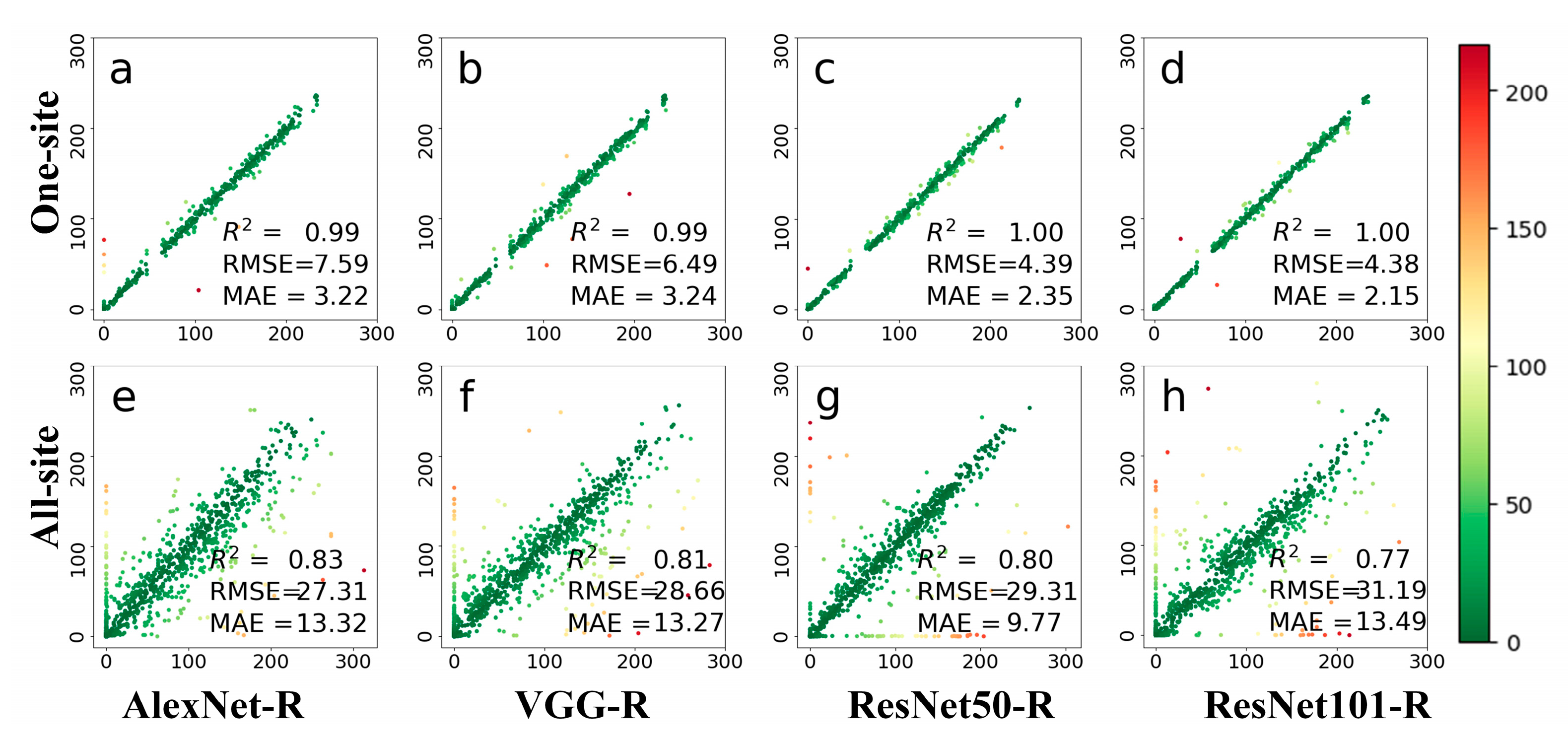
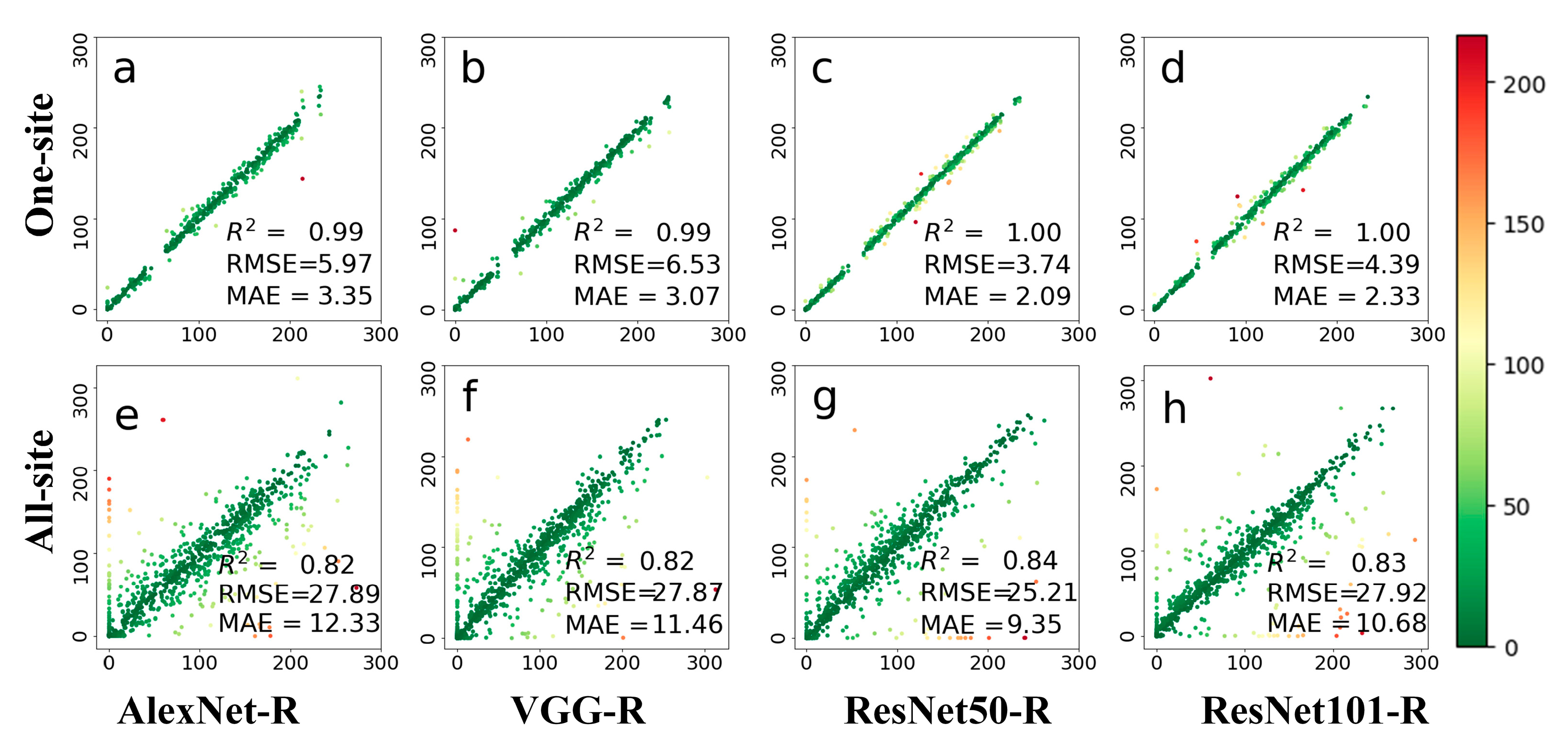
Figure 5 shows the leaf phenology prediction accuracies of the four deep learning methods on deciduous broadleaf forests at a daily scale. The four networks all show good results. All the deep networks performed well on the one-site dataset, with all results in one-site are close to the 1:1 line. PhenoCam images from the same sites have similar scenes and the same field of view. For the all-site dataset, the accuracies of four networks were reduced when using images from all-56 sites for leaf phenology prediction. The variety of colors in this figure indicates the magnitude of the prediction error, and the red ones indicate those that have the largest errors. The results for different PhenoCam images have a large deviation. In terms of the model performance, ResNet101-R achieved the best accuracy with RMSE of 4.38 days and the MAE of 2.15 days in the one-site dataset, and ResNet50-R achieved higher accuracy than the other three networks on the all-site dataset with the MAE of 9.77 days. Overall, ResNet is a robust architecture for predicting leaf growing dates among tested models.
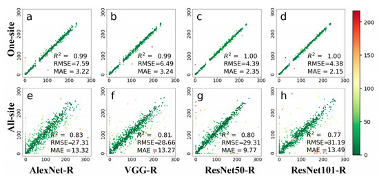
Figure 5.
Comparisons between observed and predicted daily leaf phenology using four deep networks, including AlexNet-R, VGG-R, ResNet50-R, and ResNet101-R. Phenological images from one site (top row) and all 56 sites (bottom row) were tested. The colors in this figure are indicative of prediction errors, whereas the red color indicates large errors and the green color indicates small errors. (a–d) represents the test results displayed by the four different methods at one-site; (e–h) represents the test results displayed by four methods at all-site.
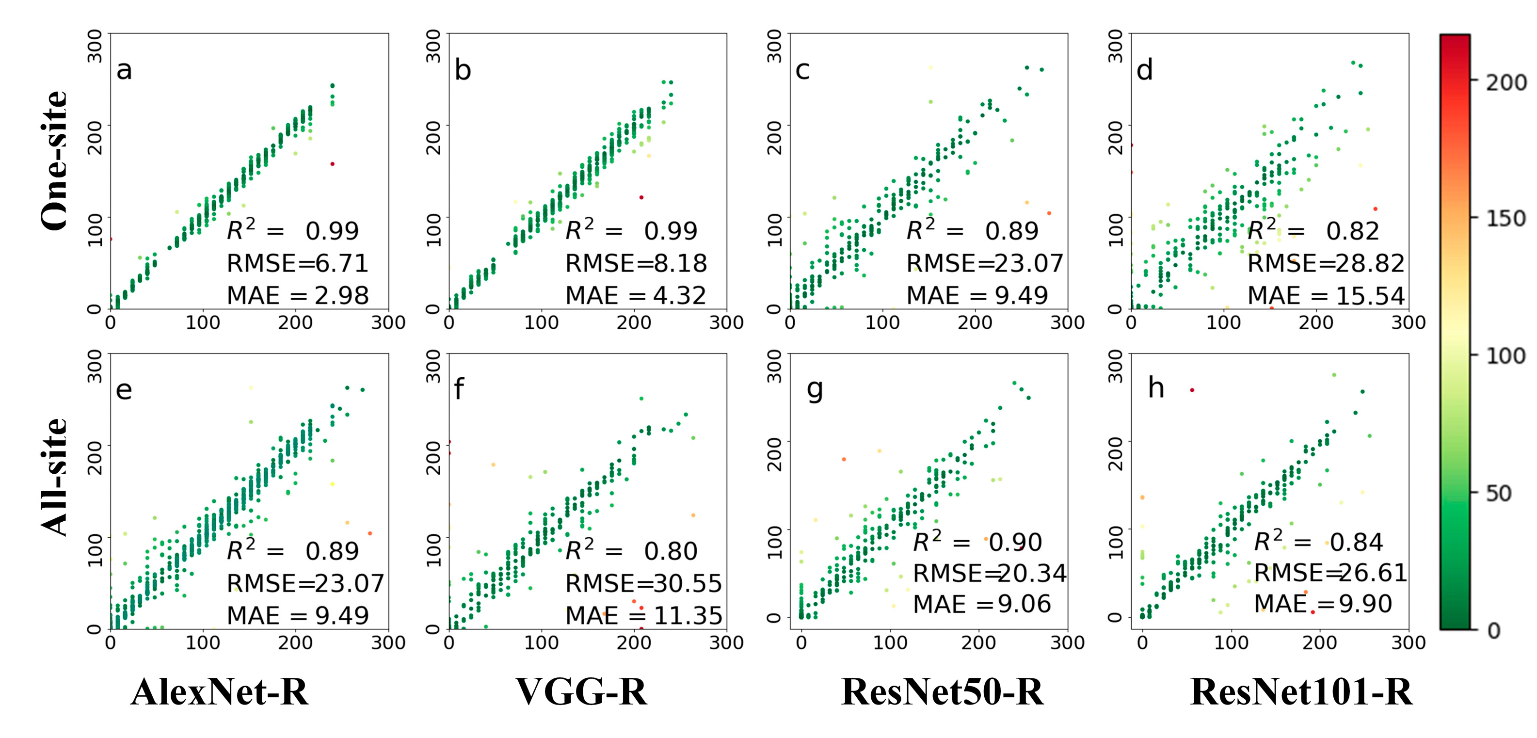
Figure 6 illustrates the results of deciduous broadleaf forests leaf phenology dates on an 8-day scale. The category of leaf phenology dates was reduced compared with that of the daily scale. A total of 636 images were verified in the first row of Figure 6. Both AlexNet-R and VGG-R achieved similar accuracies on 8-day leaf phenology prediction and daily leaf phenology in terms of R2. Compared with the other tested methods, AlexNet-R shows the best prediction results on the one-site dataset. The two ResNet architectures achieved reasonable accuracies in predicting 8-day leaf growth for the one-site dataset, and performed better for the all-site dataset. ResNet50-R achieves RMSE 10 days less than VGG-R when using the all-site dataset. It seems that ResNet is suitable for large training datasets but has overfitting issues when using small training data.
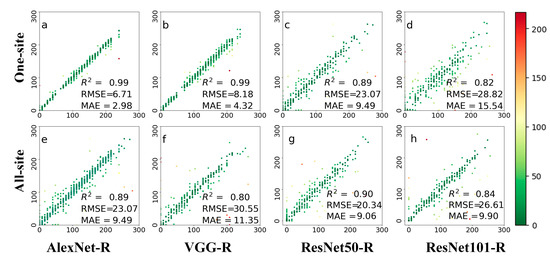
Figure 6.
The prediction results on an 8-day scale leaf phenology based on four deep networks, i.e., AlexNet-R, VGG-R, ResNet50-R, and ResNet101-R. Phenological images from one site (top row) and all 56 sites (bottom row) were tested. The colors in this figure are indicative of prediction errors, whereas the red color indicates large errors and the green color indicates small errors. (a–d) represents the test results displayed by the four different methods at one-site; (e–h) represents the test results displayed by four methods at all-site.
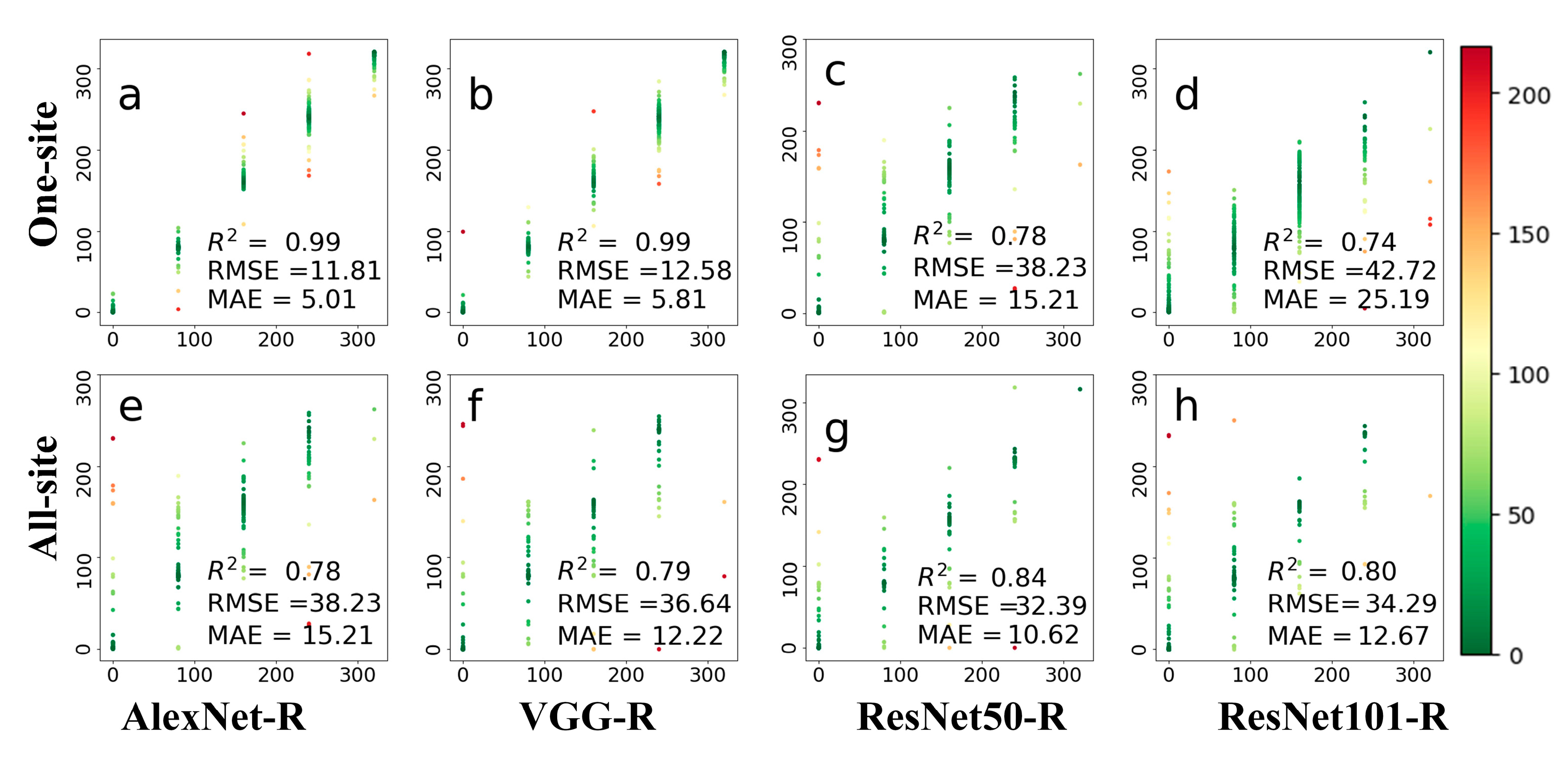
Figure 7 compares observed and predicted leaf growing dates of deciduous broadleaf forests on the 80-day scale. Compared with the experiments on both daily and 8-day time scales, there were fewer data to be tested in the 80-day experiment. The colors in this figure are indicative of prediction errors, whereas the red color indicates large errors, and the green color indicates small errors. For the one-site dataset, the AlexNet-R showed the best prediction result in terms of all metrics, with RMSE of 11.81 days and MAE of 5.01 days. When using the ResNet101-R architecture, the accuracies for the one-site dataset decrease in the 80-day experiment as compared to the 8-day experiment. For the all-site dataset, the accuracies of two ResNet architectures were improved as compared to the one-site dataset. ResNet50-R achieved accuracy with RMSE of 32.39 and MAE of 10.62.

Figure 7.
The prediction results on 80-day leaf phenology are based on four deep networks, i.e., AlexNet-R, VGG-R, ResNet50-R, and ResNet101-R. Phenological images from one site (top row) and all 56 sites (bottom row) were tested. The colors in this figure are indicative of prediction errors, whereas the red color indicates large errors, and the green color indicates small errors. (a–d) represents the test results displayed by the four different methods at one-site; (e–h) represents the test results displayed by four methods at all-site.
4.2. Predicting Leaf Phenology Using Detected ROI Images
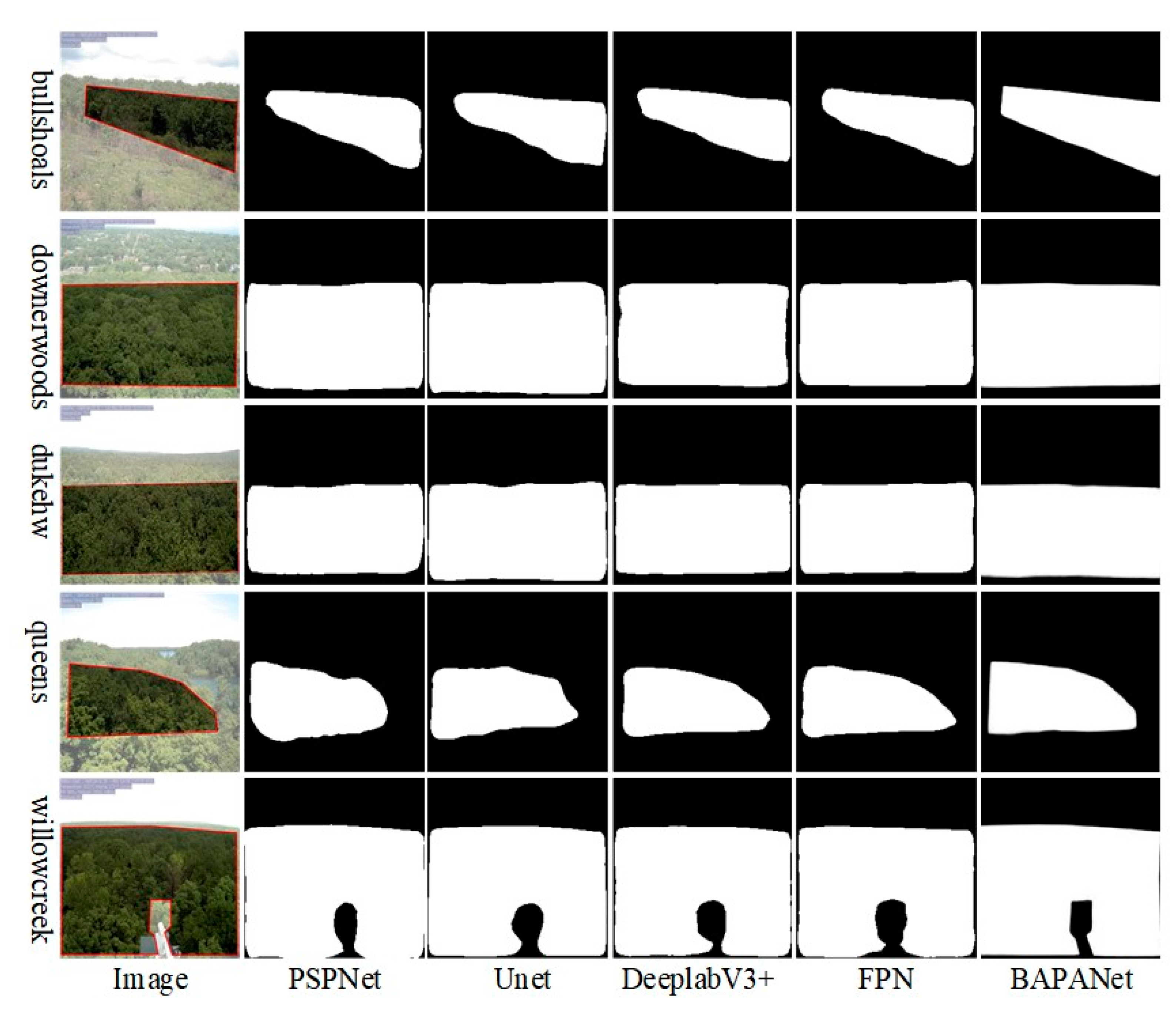
Figure 8 shows the comparison of deciduous broadleaf forest ROIs detected by five different semantic segmentation methods. Based on visual inspection, BAPANet per-formed the best among all the methods, with reasonable ROI detection results for decid-uous broadleaf forests. Compared with the other four methods, BAPANet has clearer boundaries and better segmentation details.
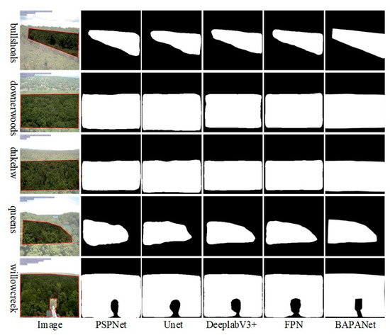
Figure 8.
Comparisons between the region of interest (ROI) of images delineated in the PhenoCam dataset and detected using different deep learning models, including PSPNet, Unet, DeeplabV3+, FPN, and BAPANet. The images are shown for five different sites, including bullshoals, downerwoods, dukehw, queens, and willowcreek. The red polygons in the images denote the ROI labelled in the PhenoCam dataset.
Image segmentation metrics are presented in Table 1. The five networks achieved similar accuracies for ROIs detection. The segmentation results of Unet and PSPNet are similar in five metrics, slightly inferior to the other three methods. The accuracies in terms of Recall, F1, and Mean IOU achieved by Unet and PSPNet are roughly 0.1 less than DeepLabV3+ and FPN, and roughly 0.2 lower than BAPANet. As shown in Table 1, BAPANet was better than the other four methods in terms of the five metrics except for the overall accuracies (0.981). In particular, the results of BAPANet were superior to other methods, with a Recall of 0.961 and F1 of 0.966.

Table 1.
The accuracy of detected ROIs using different semantic segmentation models.
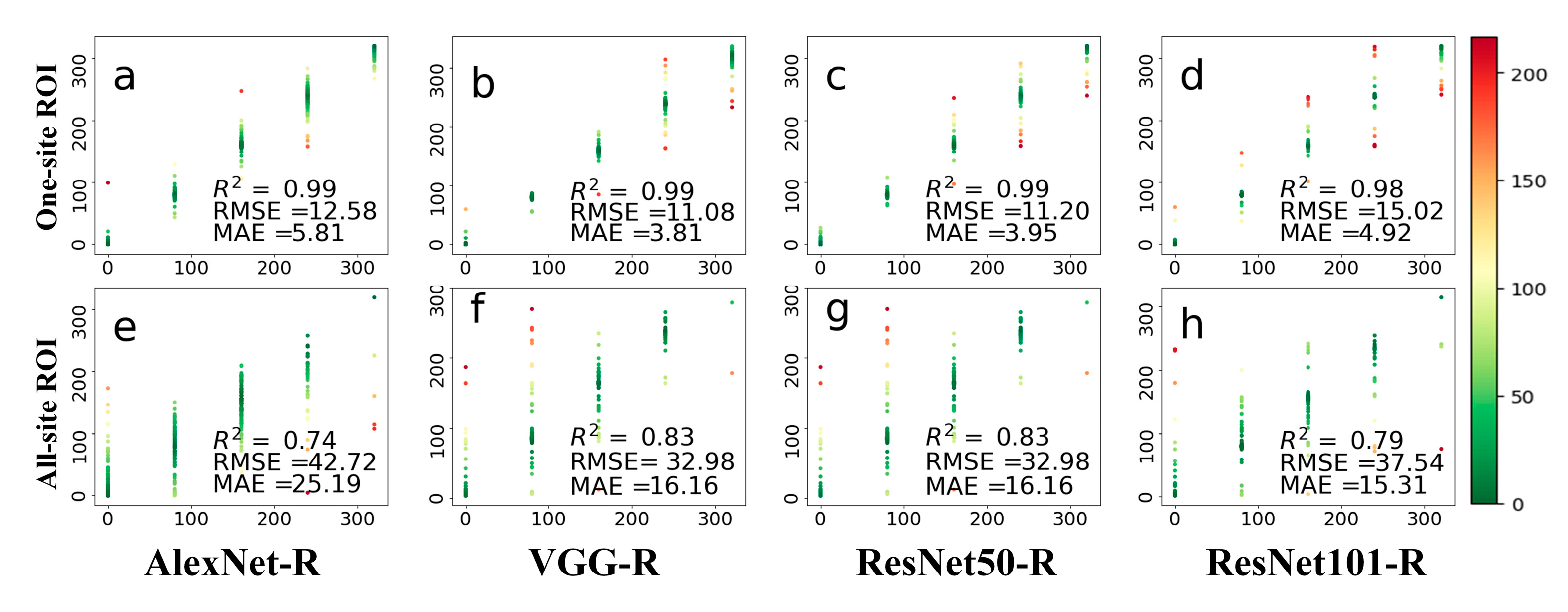
Figure 9, Figure A2 and Figure A3 show the leaf growth prediction results with the detected ROIs at three different time scales of daily, 8-day, and 80-day, respectively. Firstly, we can see that the prediction accuracies on different time scales varied greatly. The results of daily prediction accuracy were better than those of 8-day and 80-day. On the daily scale, VGG-R performed much better than AlexNet-R and two ResNet architectures for the one-site dataset, whereas the two ResNet architectures performed much better than AlexNet-R (Figure 9e) and VGG-R (Figure 9f) for the all-site dataset. For the 8-day scale (Figure A2), VGG-R achieved the best results on the one-site dataset. The RMSE was within five days, while the other methods were greater than those of the 8-day scale. On all-site datasets, the results of ResNet50-R had slightly better accuracy in terms of R2 (0.85) and RMSE (23.83). Compared with other methods, ResNet50-R achieved the best accuracy on the all-site dataset with the lowest RMSE. For the 80-day scale (Figure A3), VGG-R performed the best on the one-site dataset, followed by AlexNet and the two ResNet architectures. Again, ResNet architectures achieved better accuracies than the other deep networks. Compared with using the whole PhenoCam image, VGG-R method has better prediction results with the detected ROIs input, both on one-site and all-site datasets. ResNet50-R has a slight advantage on daily and 8-day leaf growth prediction based on the detected ROIs. Similar results were obtained with the 80-day time scale. In general, the second strategy performed better than the first one, and ROIs could remove the interference by other information (such as the sky or other land covers) in the PhenoCam image.
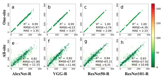
Figure 9.
Comparison of four methods (AlexNet-R, VGG-R, ResNet50-R, and ResNet101-R) on the daily prediction results after ROI segmented by BAPANet. Both phenological images and ROIs from one site and all 56 sites were tested. The two rows represent a single site and all sites, respectively. The green dot indicates that the prediction result was better, and the color result values of red, green, and blue decreased successively. (a–d) represents the test results displayed by the four different methods at one-site; (e–h) represents the test results displayed by four methods at all-site.
5. Discussion
Based on the results above, we found that the results of leaf phenology prediction vary greatly when using the one-site and all-site datasets. By comparing the results obtained from the one-site and all-site datasets, we found that the convolutional neural network regression methods used in this paper performed well when predicting the results of a single site, but need improvements when applied to multiple sites. One possible reason is that images from different sites vary largely due to imaging conditions, making it difficult for training and convergence of the deep learning models.
The accuracy of leaf phenology prediction also depends on the training dataset. Imaging conditions and observation frequency often vary considerably from site to site, leading to the variation of data distribution. For most of the studied sites, vegetation leaf comes out in spring and falls off in autumn, whereas there are high-altitude sites where vegetation leaf comes out in summer or even autumn with a much shorter growing period. These altitude and latitude conditions lead to a wide variation in the prediction of leaf phenology from site to site and result in phenology prediction errors. From the presented results, we found that different network structures lead to large differences in the predicted results. In addition to the network architecture, training data is one important factor that influences the performance of deep learning models. Collecting observation datasets from sites with varying altitudes and latitudes are likely useful for improving the applicability of the deep learning models.
According to the results, we found that the accuracies of leaf phenology prediction varied largely with the time scales. The experimental results showed that the models performed better on the daily scale than on the 8-day or 80-day scales. In addition, the R2 showed that the model performed better on the 8-day scale than those on the 80-day scale, especially at multiple sites. For the 8-day and 80-day scales, VGG-R and AlexNet achieved better results in the one-site datasets than in the all-site dataset. For the daily time scale, Resnet-50 performed well on both one-site and all-site datasets. In the experiments at different time scales using the all-site dataset, the two ResNet architectures performed relatively better than the other methods. Overall, the daily time scale is a reasonable scale for leaf phenology prediction. It is probably the case that the uncertainties related to series generation are too coarse in 8-day and 80-day scales for the accurate estimation of the leaf growth between EOS and SOS. As the results show in Figure 5 and Figure 9, we predicted leaf phenology on the daily scale from the entire PhenoCam image, as well as the detected ROI images. Compared with the first strategy, the accuracy of the second strategy that used ROIs as model inputs slightly improved. The two ResNet-R structures achieved slightly better accuracies using ROIs than using the entire PhenoCam images to predict daily leaf phenology based on the one-site dataset. Both AlexNet-R and VGG-R also reduce RMSE errors when using ROIs as compared with using entire PhenoCam images as model inputs. This implies that detecting ROI images helps phenology prediction as the use of ROIs reduces irrelevant but influential backgrounds other than vegetation canopies.
Different layers of networks have different advantages in leaf growth prediction. The shallow networks such as AlexNet-R achieved better accuracies on the 8-day and 80-day scales in the one-site dataset. The method of VGG-R using the detected ROIs has advantages in the one-site dataset compared to the deep network. Deeper networks such as ResNet50-R and ResNet101-R performed better in the all-site dataset. The deep network of ResNet with 50 layers performed better than that with 101 layers. This implies that deep networks are suitable for complex data processing, and high-level features extracted by deeper networks likely lead to overfitting when the dataset comes from only one site. Overall, increasing the network depth does not always improve the accuracies in predicting leaf growing dates directly from the PhenoCam images, and finding a suitable network is important for leaf phenology prediction.
In addition, there are still some improvements that can be made in future studies. For example, we might integrate the ROI detection network and the phenology prediction network together to improve the model performance and computational efficiency. On the other hand, we would add other indices (such as LAI, NDVI, etc.) to improve the identification of leaf phenology.
6. Conclusions
This study investigated the ability of four deep learning models to identify leaf phenology from individual PhenoCam images. The deep learning models can extract high-level features from high-frequency PhenoCam images, making it a special solution for leaf phenology prediction. Compared to the existing methods that analyze leaf phenology using time series of PhenoCam images, our algorithm is able to predict leaf phenology from one PhenoCam image only. The accuracy in terms of MAE is about two days at a single site, and that of multiple sites is about 9 days. The two ResNet architectures performed better than the other two methods on the multiple sites test dataset. Although we take deciduous broad-leaved forest as the studied plant functional type, it is possible that the method developed can be extended to other vegetation types such as crops, and crop leaf phenology prediction will thus provide efficient and effective possibilities for crop yield estimation. While challenges in accurate identification of leaf phenology from digital camera photos remain, we provide a feasible solution to predict daily leaf phenology using individual PhenoCam images via deep learning.
Author Contributions
Conceptualization, M.C., Y.S., X.J., Z.L., and Q.X.; pre-processing, M.C.; methodology, M.C., Z.L.; conceived, M.C., Q.X.; software, M.C., X.J.; resources, Q.X.; writing—original draft preparation, M.C.; writing—review and editing, Y.S., Q.X., X.J.; supervision, Y.S., Q.X.; funding acquisition, Y.S., Q.X. All authors have read and agreed to the published version of the manuscript.
Funding
This research was supported by National Key R&D Program of China (grant no. 2017YFA0604300 and 2017YFA0604400), National Natural Science Foundation of China (grant no. 41875122) and Natural Science Foundation of Guangdong Province (grant no. 2021A1515011429). Program of the National Natural Science Foundation of China (grant no. 41801351) and Natural Science Foundation of Guangdong Province (grant no. 2021A1515011429). We also thank anonymous reviewers for their constructive comments.
Data Availability Statement
PhenoCam Images are available at https://phenocam.sr.unh.edu/webcam/network/download/; accessed on 18 September 2020. ROI dataset is available at https://phenocam.sr.unh.edu/webcam/roi/search/ accessed on 18 September 2020). The label and GCC files are available at https://daac.ornl.gov/cgi-bin/dsviewer.pl?ds_id=1511; accessed on 20 September 2020. The scripts used to generate all the results are at https://github.com/caomy7/leaf-phenology; accessed on 13 May 2021. Analysis scripts are available on request from https://github.com/caomy7/leaf-phenology/edit/main/README.md accessed on 13 May 2021.
Acknowledgments
We thank the researchers and investigators who are involved in collecting and sharing the PhenoCam dataset.
Conflicts of Interest
The authors declare that they have no conflict of interest.
Appendix A

Table A1.
The sample information of the 56 sites. We selected one year of the PhenoCam images at each site for analysis, and the vegetation types are deciduous broad-leaved forests.
Table A1.
The sample information of the 56 sites. We selected one year of the PhenoCam images at each site for analysis, and the vegetation types are deciduous broad-leaved forests.
| Site Name | Latitude (°) | Longitude (°) | Elevation (M) | SOS (Star-of-Season) | EOS (Star-of-Season) | Image Number and the Year |
|---|---|---|---|---|---|---|
| Acadia | 44.3769 | −68.2608 | 158 | 2016/5/8 | 2016/10/21 | 338/2016 |
| Alligatorriver | 35.7879 | −75.9038 | 1 | 2016/3/27 | 2016/10/16 | 285/2016 |
| Asa | 57.1645 | 14.7825 | 180 | 2015/5/23 | 2015/10/28 | 186/2015 |
| Bartlett | 44.0646 | −71.2881 | 268 | 2015/4/10 | 2015/11/6 | 297/2015 |
| Bartlettir | 44.0646 | −71.2881 | 268 | 2016/5/10 | 2016/11/26 | 353/2016 |
| Bitterootvalley | 46.5070 | −114.0910 | 1017 | 2016/5/9 | 2016/10/7 | 357/2016 |
| Bostoncommon | 42.3559 | −71.0641 | 10 | 2016/4/9 | 2016/10/27 | 157/2016 |
| Boundarywaters | 47.9467 | −91.4955 | 519 | 2016/4/25 | 2016/11/21 | 350/2016 |
| Bullshoals | 36.5628 | −93.0666 | 260 | 2016/5/19 | 2016/9/25 | 315/2016 |
| Canadaoa | 53.6289 | −106.1978 | 601 | 2016/4/1 | 2016/11/13 | 212/2016 |
| Caryinstitute | 41.7839 | −73.7341 | 127 | 2016/5/1 | 2016/6/4 | 347/2016 |
| Cedarcreek | 45.4019 | −93.2042 | 276 | 2016/5/1 | 2016/10/30 | 288/2016 |
| Columbiamissouri | 38.7441 | −92.1997 | 232 | 2009/4/11 | 2009/11/9 | 144/2009 |
| Coweeta | 35.0596 | −83.4280 | 680 | 2016/4/8 | 2016/10/20 | 291/2016 |
| Dollysods | 39.0995 | −79.4270 | 1133 | 2003/4/21 | 2003/11/2 | 230/2003 |
| Downerwoods | 43.0794 | −87.8808 | 213 | 2016/5/8 | 2016/10/21 | 339/2016 |
| Drippingsprings | 33.3000 | −116.8000 | 400 | 2006/4/2 | 2006/12/29 | 364/2006 |
| Dukehw | 35.9736 | −79.1004 | 400 | 2016/3/12 | 2016/10/31 | 329/2016 |
| Harvard | 42.5378 | −72.1715 | 340 | 2016/5/6 | 2016/10/27 | 359/2016 |
| Harvardbarn2 | 42.5353 | −72.1899 | 350 | 2016/5/9 | 2016/10/21 | 360/2016 |
| Harvardlph | 42.5420 | −72.1850 | 380 | 2016/5/10 | 2016/10/20 | 357/2016 |
| Howland2 | 45.2128 | −68.7418 | 79 | 2016/5/21 | 2016/10/4 | 206/2016 |
| Hubbardbrook | 43.9438 | −71.7010 | 253 | 2016/5/2 | 2016/11/6 | 351/2016 |
| Hubbardbrooknfws | 42.9580 | −71.7762 | 930 | 2016/5/21 | 2016/10/9 | 73/2016 |
| Joycekilmer | 35.2570 | −83.7950 | 1373 | 2016/4/26 | 2016/10/20 | 314/2016 |
| Laurentides | 45.9881 | −74.0055 | 350 | 2016/5/16 | 2016/10/8 | 354/2016 |
| Mammothcave | 37.1858 | −86.1019 | 226 | 2016/3/31 | 2016/10/29 | 336/2016 |
| Missouriozarks | 38.7441 | −92.2000 | 219 | 2016/4/15 | 2016/10/30 | 319/2016 |
| Monture | 47.0202 | −113.1283 | 1255 | 2007/4/29 | 2007/10/13 | 274/2007 |
| Morganmonroe | 39.3231 | −86.4131 | 275 | 2016/4/10 | 2016/11/3 | 345/2016 |
| Nationalcapital | 38.8882 | −77.0695 | 28 | 2016/3/19 | 2016/11/14 | 269/2016 |
| Northattleboroma | 41.9837 | −71.3106 | 60 | 2016/5/4 | 2016/10/18 | 349/2016 |
| Oakridge1 | 35.9311 | −84.3323 | 371 | 2016/3/26 | 2016/5/26 | 182/2016 |
| Oakridge2 | 35.9311 | −84.3323 | 371 | 2016/3/27 | 2016/5/28 | 182/2016 |
| Proctor | 44.5250 | −72.8660 | 403 | 2016/5/10 | 2016/10/18 | 353/2016 |
| Queens | 44.5650 | −76.3240 | 126 | 2016/5/8 | 2016/10/16 | 347/2016 |
| Readingma | 42.5304 | −71.1272 | 100 | 2016/4/22 | 2016/11/7 | 348/2016 |
| Russellsage | 32.4570 | −91.9743 | 20 | 2016/3/17 | 2016/11/29 | 320/2016 |
| Sanford | 42.7268 | −84.4645 | 268 | 2016/4/22 | 2016/11/2 | 364/2016 |
| Shalehillsczo | 40.6500 | −77.9000 | 310 | 2016/4/23 | 2016/10/28 | 278/2016 |
| Shiningrock | 35.3902 | −82.7750 | 1500 | 2006/5/12 | 2006/10/18 | 313/2006 |
| Silaslittle | 39.9137 | −74.5960 | 33 | 2016/12/6 | 2016/10/28 | 247/2016 |
| Smokylook | 35.6325 | −83.9431 | 801 | 2016/4/16 | 2016/10/22 | 333/2016 |
| Smokypurchase | 35.5900 | −83.0775 | 1550 | 2016/4/22 | 2016/10/18 | 342/2016 |
| Snakerivermn | 46.1206 | −93.2447 | 1181 | 2016/5/9 | 2016/10/4 | 263/2016 |
| Springfieldma | 42.1352 | −72.5860 | 56 | 2016/11/8 | 2016/11/1 | 318/2016 |
| Thompsonfarm2n | 43.1086 | −70.9505 | 23 | 2016/3/25 | 2016/12/4 | 322/2016 |
| Tonzi | 38.4309 | −120.9659 | 177 | 2016/2/28 | 2016/6/13 | 252/2016 |
| Turkeypointdbf | 42.6353 | −80.5576 | 211 | 2016/5/11 | 2016/10/18 | 298/2016 |
| Umichbiological | 45.5598 | −84.7138 | 230 | 2016/5/16 | 2016/10/21 | 347/2016 |
| Umichbiological2 | 45.5625 | −84.6976 | 240 | 2016/5/8 | 2016/10/19 | 336/2016 |
| Upperbuffalo | 35.8637 | −93.4932 | 777 | 2006/4/8 | 2006/10/19 | 257/2006 |
| Uwmfieldsta | 43.3871 | −88.0229 | 265 | 2016/5/5 | 2016/10/22 | 344/2016 |
| Willowcreek | 45.8060 | −90.0791 | 521 | 2016/5/7 | 2016/10/3 | 307/2016 |
| Woodshole | 41.5495 | −70.6432 | 10 | 2016/5/8 | 2016/11/1 | 288/2016 |
| Worcester | 42.2697 | −71.8428 | 185 | 2016/4/22 | 2016/10/20 | 353/2016 |
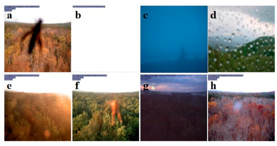
Figure A1.
The PhenoCam data that has been eliminated by manual screening. (a) refers to the lens pollution by animal or other tracks, (b) refers to the camera signal error, (c) refers to the influence of dense fog, and (d) refers to the interference of a large amount of water droplets. (e–h) is the interference of the solar light spots and scattering to the lens.

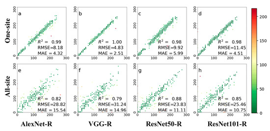
Figure A2.
Compared four methods (AlexNet-R, VGG-R, ResNet50-R, and ResNet101-R) on the 8-day prediction results after ROI segmented by BAPANet. Both phenological images and ROIs from one site and all 56 sites were tested. From top to bottom, represents a single site and all sites. The green dot indicates that the prediction result is better, and the color result values of red, green and blue decrease successively. (a–d) represents the test results displayed by the four different methods at one-site; (e–h) represents the test results displayed by four methods at all-site.
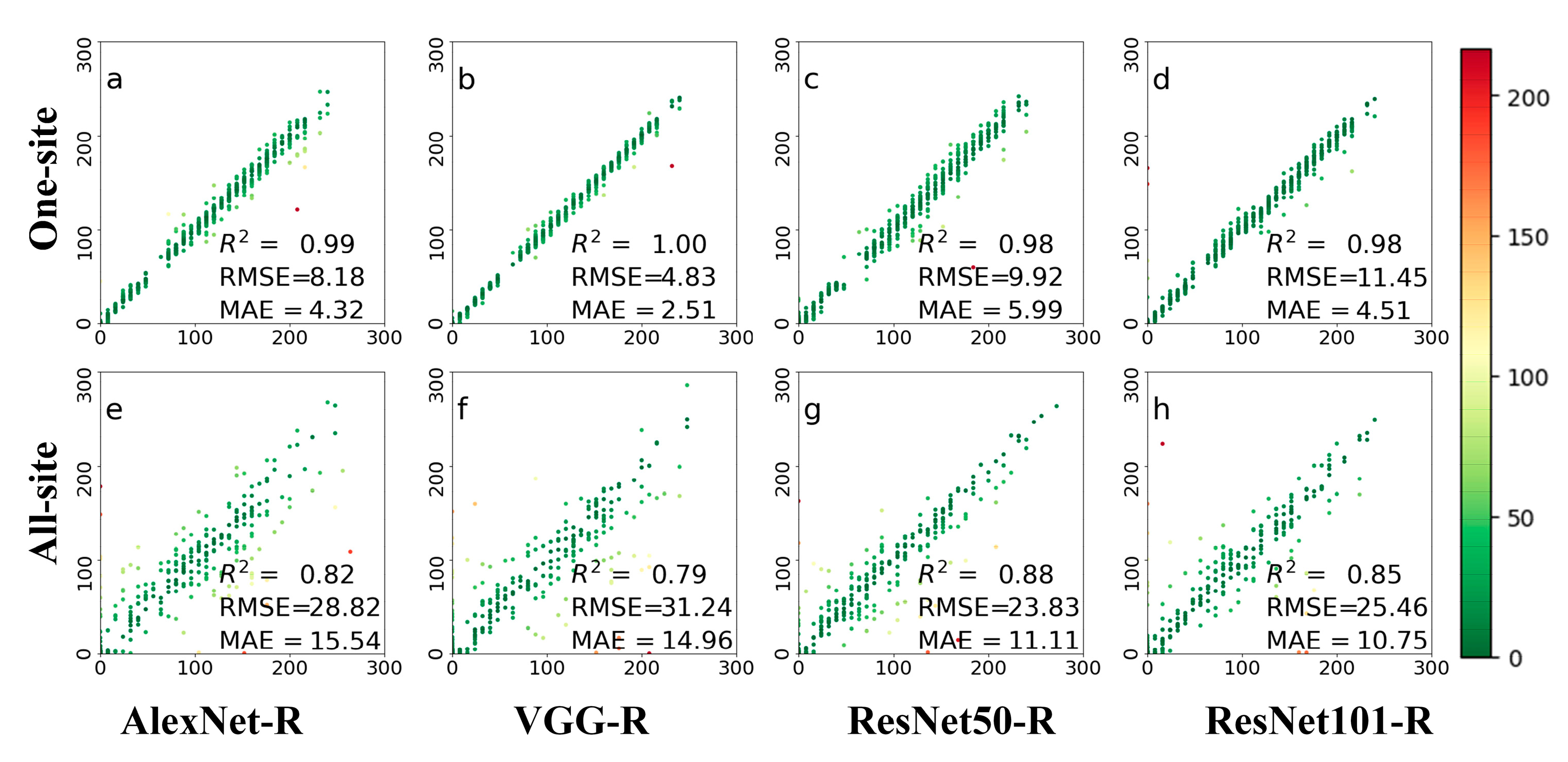
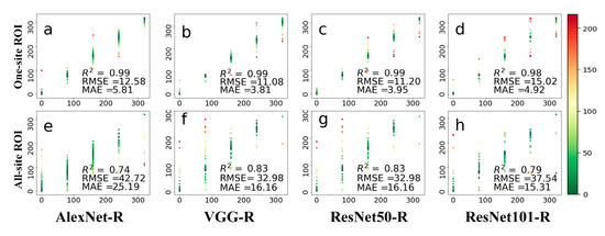
Figure A3.
The prediction results on 80-day leaf phenology are based on four deep networks (AlexNet-R, VGG-R, ResNet50-R, and ResNet101-R). Both phenological images from one site (top row) and all 56 sites (bottom row) were tested. The colors in this figure are indicative to prediction errors, whereas red color indicates large errors and green color indicates small errors. (a–d) represents the test results displayed by the four different methods at one-site; (e–h) represents the test results displayed by four methods at all-site.
References
- Liu, Y.; Wu, C.Y.; Sonnentag, O.; Desai, A.R.; Wang, J. Using the red chromatic coordinate to characterize the phenology of forest canopy photosynthesis. Agric. For. Meteorol. 2020, 285–286, 107910. [Google Scholar] [CrossRef]
- Fitter, A.H.; Fitter, R.S.R. Rapid changes in flowering time in British plants. Science 2002, 296, 1689–1691. [Google Scholar] [CrossRef] [PubMed]
- Menzel, A. Phenology: Its importance to the global change community—An editorial comment. Clim. Change 2002, 54, 379–385. [Google Scholar] [CrossRef]
- Morisette, J.T.; Richardson, A.D.; Knapp, A.K.; Fisher, J.I.; Graham, E.A.; Abatzoglou, J.; Wilson, B.E.; Breshears, D.D.; Henebry, G.M.; Hanes, J.M.; et al. Tracking the rhythm of the seasons in the face of global change: Phenological research in the 21st century. Front. Ecol. Environ. 2009, 7, 253–260. [Google Scholar] [CrossRef]
- Richardson, A.D.; Klosterman, S.; Toomey, M. Near-Surface Sensor-Derived Phenology. Phenology: An Integrative Environmental Science; Springer: Berlin/Heidelberg, Germany, 2013; pp. 413–430. [Google Scholar]
- Hogg, E.H.; Price, D.T.; Black, T.A. Postulated feedbacks of deciduous forest phenology on seasonal climate patterns in the western Canadian interior. J. Clim. 2000, 13, 4229–4243. [Google Scholar] [CrossRef]
- Xin, Q.C.; Zhou, X.W.; Wei, N.; Yuan, H.; Ao, Z.R.; Dai, Y.J. A semiprognostic phenology model for simulating multidecadal dynamics of global vegetation leaf area index. J. Adv. Model. Earth Syst. 2020, 12, e2019MS001935. [Google Scholar] [CrossRef]
- Kikuzawa, K. Leaf phenology as an optimal strategy for carbon gain in plants. Can. J. Bot. 1995, 73, 158–163. [Google Scholar] [CrossRef]
- Luo, Y.P.; El-Madany, T.S.; Filippa, G.; Ma, X.L.; Ahrens, B.; Carrara, A.; Gonzalez-Cascon, R.; Cremonese, E.; Galvagno, M.; Hammer, T.W.; et al. Using Near-Infrared-Enabled Digital Repeat Photography to Track Structural and Physiological Phenology in Mediterranean Tree–Grass Ecosystems. Remote Sens. 2018, 10, 1293. [Google Scholar] [CrossRef]
- Fisher, J.I.; Mustard, J.F.; Vadeboncoeur, M.A. Green leaf phenology at Landsat resolution: Scaling from the field to the satellite. Remote Sens. Environ. 2006, 100, 265–279. [Google Scholar] [CrossRef]
- Sparks, T.H.; Menzel, A. Observed changes in seasons: An overview. Int. J. Climatol. 2002, 22, 1715–1725. [Google Scholar] [CrossRef]
- White, M.A.; Thornton, P.E.; Runnin, S.W. A continental phenology model for monitoring vegetation responses to interannual climatic variability. Glob. Biogeochem. Cycles 1997, 11, 217–234. [Google Scholar] [CrossRef]
- Justice, C.O.; Townshend, J.R.G.; Holben, B.N.; Tucker, C.J. Analysis of the phenology of global vegetation using meteorological satellite data. Int. J. Remote Sens. 1985, 6, 1271–1318. [Google Scholar] [CrossRef]
- Zhang, X.Y.; Friedl, M.A.; Schaaf, C.B.; Strahler, A.H.; Hodges, J.C.F.; Gao, F.; Reed, B.C.; Huete, A. Monitoring vegetation phenology using MODIS. Remote Sens. Environ. 2003, 84, 471–475. [Google Scholar] [CrossRef]
- Hilker, T.; Wulder, M.A.; Coops, N.C.; Linke, J.; McDermid, G.; Masek, J.G.; Gao, F.; White, J.C. A new data fusion model for high spatial- and temporal-resolution mapping of forest disturbance based on Landsat and MODIS. Remote Sens. Environ. 2009, 113, 1613–1627. [Google Scholar] [CrossRef]
- Badeck, F.W.; Bondeau, A.; Bottcher, K.; Doktor, D.; Lucht, W.; Schaber, J.; Sitch, S. Responses of spring phenology to climate change. New Phytol. 2004, 162, 295–309. [Google Scholar] [CrossRef]
- Richardson, A.D. Tracking seasonal rhythms of plants in diverse ecosystems with digital camera imagery. New Phytol. 2019, 222, 1742–1750. [Google Scholar] [CrossRef] [PubMed]
- Brown, T.B.; Hultine, K.R.; Steltzer, H.; Denny, E.G.; Denslow, M.W.; Granados, J.; Henderson, S.; Moore, D.; Nagai, S.; SanClements, M.; et al. Using phenocams to monitor our changing Earth: Toward a global phenocam network. Front. Ecol. Environ. 2016, 14, 84–93. [Google Scholar] [CrossRef]
- Bornez, K.; Richardson, A.D.; Verger, A.; Descals, A.; Penuelas, J. Evaluation of vegetation and proba-v phenology using phenocam and eddy covariance data. Remote Sens. 2020, 12, 3077. [Google Scholar] [CrossRef]
- Richardson, A.D.; Hufkens, K.; Milliman, T.; Frolking, S. Intercomparison of phenological transition dates derived from the PhenoCam Dataset V1.0 and MODIS satellite remote sensing. Sci. Rep. 2018, 8, 5679. [Google Scholar] [CrossRef] [PubMed]
- Wang, H.S.; Jia, G.S.; Epstein, H.E.; Zhao, H.C.; Zhang, A.Z. Integrating a PhenoCam-derived vegetation index into a light use efficiency model to estimate daily gross primary production in a semi-arid grassland. Agric. For. Meteorol. 2020, 288–289, 107983. [Google Scholar] [CrossRef]
- Wu, J.; Rogers, A.; Albert, L.P.; Ely, K.; Prohaska, N.; Wolfe, B.T.; Oliveira, R.C.; Saleska, S.R.; Serbin, S.P. Leaf reflectance spectroscopy captures variation in carboxylation capacity across species, canopy environment and leaf age in lowland moist tropical forests. New Phytol. 2019, 224, 663–674. [Google Scholar] [CrossRef] [PubMed]
- Zhang, X.Y.; Jayavelu, S.; Liu, L.L.; Friedl, M.A.; Henebry, G.M.; Liu, Y.; Schaaf, C.B.; Richardson, A.D.; Gray, J. Evaluation of land surface phenology from VIIRS data using time series of PhenoCam imagery. Agric. For. Meteorol. 2018, 256, 137–149. [Google Scholar] [CrossRef]
- Zhang, S.K.; Butto, V.; Khare, S.; Deslauriers, A.; Morin, H.; Huang, J.G.; Ren, H.; Rossi, S. Calibrating PhenoCam Data with Phenological Observations of a Black Spruce Stand. Can. J. Remote Sens. 2020, 46, 154–165. [Google Scholar] [CrossRef]
- LeCun, Y.; Bengio, Y.; Hinton, G. Deep learning. Nature 2015, 521, 436–444. [Google Scholar] [CrossRef]
- Richardson, A.D.; Hufkens, K.; Milliman, T.; Aubrecht, D.M.; Chen, A.; Gray, J.M.; Johnston, M.R.; Keenan, T.F.; Klosterman, S.T.; Kosmala, M.; et al. Tracking vegetation phenology across diverse North American biomes using PhenoCam imagery. Sci. Data 2018, 5, 1–24. [Google Scholar] [CrossRef]
- Sonnentag, O.; Hufkens, K.; Teshera-Sterne, C.; Young, A.M.; Friedl, M.; Braswell, B.H.; Milliman, T.; O’Keefe, J.; Richardson, A.D. Digital repeat photography for phenological research in forest ecosystems. Agric. For. Meteorol. 2012, 152, 159–177. [Google Scholar] [CrossRef]
- Seyednasrollah, B.; Young, A.M.; Hufkens, K.; Milliman, T.; Friedl, M.A.; Frolking, S.; Richardson, A.D. Tracking vegetation phenology across diverse biomes using Version 2.0 of the PhenoCam Dataset. Sci. Data 2019, 6, 222. [Google Scholar] [CrossRef]
- Krizhevsky, A.; Sutskever, I.; Hinton, G.E. Alexnet Imagenet classification with deep convolutional neural networks. Adv. Neural Info Process. Syst. 2012, 25, 1097–1105. [Google Scholar]
- Simonyan, K.; Zisserman, A. Very deep convolutional networks for large-scale image recognition. arXiv 2014, arXiv:1409.1556. [Google Scholar]
- Szegedy, C.; Liu, W.; Jia, Y.; Sermanet, P.; Reed, S.; Anguelov, D.; Erhan, D.; Vanhoucke, V.; Rabinovich, A. Going Deeper with Convolutions. In Proceedings of the 2015 IEEE Conference on Computer Vision and Pattern Recognition (CVPR), Boston, MA, USA, 7–12 June 2015; pp. 1–9. [Google Scholar]
- He, K.; Zhang, X.; Ren, S.; Sun, J. Deep residual learning for image recognition. In Proceedings of the 2016 IEEE Conference on Computer Vision and Pattern Recognition (CVPR), Las Vegas, NV, USA, 27–30 June 2016; pp. 770–778. [Google Scholar]
- Ma, L.; Shuai, R.J.; Ran, X.M.; Liu, W.J.; Ye, C. Combining DC-GAN with ResNet for blood cell image classification. Med. Biol. Eng. Comput. 2020, 58, 1251–1264. [Google Scholar] [CrossRef]
- Long, J.; Shelhamer, E.; Darrell, T. Fully convolutional networks for semantic segmentation. In Proceedings of the 2015 IEEE Conference on Computer Vision and Pattern Recognition (CVPR), Boston, MA, USA, 7–12 June 2015; pp. 3431–3440. [Google Scholar]
- Badrinarayanan, V.; Kendall, A.; Cipolla, R. Segnet: A deep convolutional encoder-decoder architecture for image segmentation. IEEE Trans. Pattern Analy. Mach. Intel. 2017, 39, 2481–2495. [Google Scholar] [CrossRef]
- Lalli, P.; Murphey, C.L.; Kucheryavaya, A.Y.; Bray, R.A. Evaluation of discrepant deceased donor hla typings reported in Unet. Hum. Immunol. 2017, 78, 92. [Google Scholar] [CrossRef]
- Chen, L.C.; Papandreou, G.; Kokkinos, I.; Murphy, K.; Yuille, A.L. Deeplab: Semantic image segmentation with deep convolutional nets, atrous convolution, and fully connected crfs. IEEE Trans. Pattern Analy. Mach. Intel. 2018, 40, 834–848. [Google Scholar] [CrossRef] [PubMed]
- Zhou, J.C.; Hao, M.L.; Zhang, D.H.; Zou, P.Y.; Zhang, W.S. Fusion PSPnet Image Segmentation Based Method for Multi-Focus Image Fusion. IEEE Photonics J. 2019, 11, 1–12. [Google Scholar] [CrossRef]
- Jiang, X.; Zhang, X.C.; Xin, Q.C.; Xi, X.; Zhang, P.C. Arbitrary-Shaped Building Boundary-Aware Detection with Pixel Aggregation Network. IEEE J. Sel. Top. App. Remote Sens. 2020. [Google Scholar] [CrossRef]
- Willmott, C.J.; Ackleson, S.G.; Davis, R.E.; Feddema, J.J.; Klink, K.M.; Legates, D.R.; O’Donnell, J.; Rowe, C.M. Statistics for the evaluation and comparison of models. J. Geophys. Res. 1985, 90, 8995–9005. [Google Scholar] [CrossRef]
Publisher’s Note: MDPI stays neutral with regard to jurisdictional claims in published maps and institutional affiliations. |
© 2021 by the authors. Licensee MDPI, Basel, Switzerland. This article is an open access article distributed under the terms and conditions of the Creative Commons Attribution (CC BY) license (https://creativecommons.org/licenses/by/4.0/).

