Article

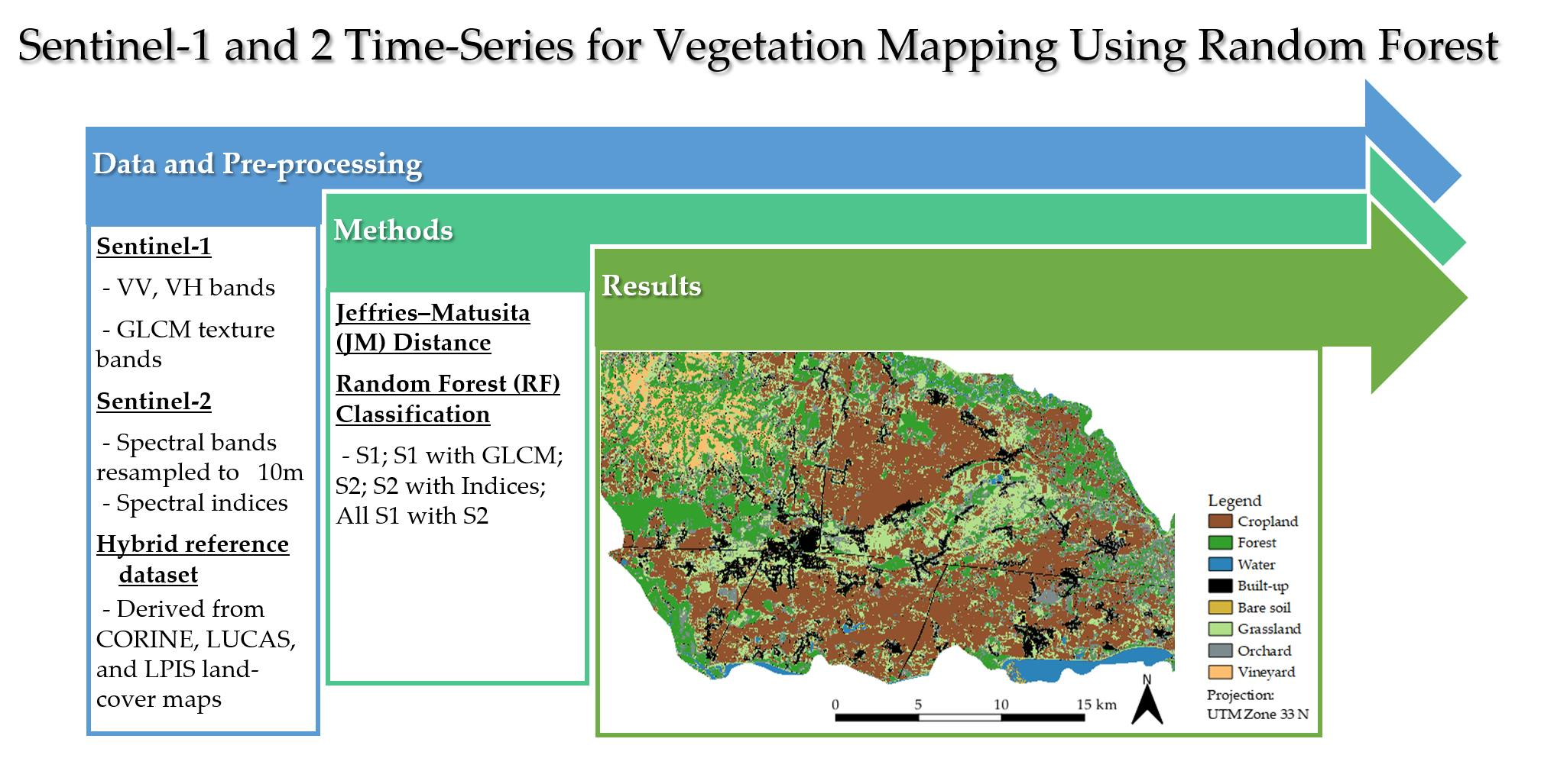
Sentinel-1 and 2 Time-Series for Vegetation Mapping Using Random Forest Classification: A Case Study of Northern Croatia

1
Chair of Geoinformatics, Faculty of Geodesy, University of Zagreb, 10000 Zagreb, Croatia
2
Chair of Photogrammetry and Remote Sensing, Faculty of Geodesy, University of Zagreb, 10000 Zagreb, Croatia
*
Author to whom correspondence should be addressed.
Remote Sens. 2021, 13(12), 2321; https://doi.org/10.3390/rs13122321
Submission received: 12 May 2021 / Revised: 9 June 2021 / Accepted: 10 June 2021 / Published: 13 June 2021
(This article belongs to the Special Issue Multi-Sensor Systems and Data Fusion in Remote Sensing)

Abstract

:
Land-cover (LC) mapping in a morphologically heterogeneous landscape area is a challenging task since various LC classes (e.g., crop types in agricultural areas) are spectrally similar. Most research is still mostly relying on optical satellite imagery for these tasks, whereas synthetic aperture radar (SAR) imagery is often neglected. Therefore, this research assessed the classification accuracy using the recent Sentinel-1 (S1) SAR and Sentinel-2 (S2) time-series data for LC mapping, especially vegetation classes. Additionally, ancillary data, such as texture features, spectral indices from S1 and S2, respectively, as well as digital elevation model (DEM), were used in different classification scenarios. Random Forest (RF) was used for classification tasks using a proposed hybrid reference dataset derived from European Land Use and Coverage Area Frame Survey (LUCAS), CORINE, and Land Parcel Identification Systems (LPIS) LC database. Based on the RF variable selection using Mean Decrease Accuracy (MDA), the combination of S1 and S2 data yielded the highest overall accuracy (OA) of 91.78%, with a total disagreement of 8.22%. The most pertinent features for vegetation mapping were GLCM Mean and Variance for S1, NDVI, along with Red and SWIR band for S2, whereas the digital elevation model produced major classification enhancement as an input feature. The results of this study demonstrated that the aforementioned approach (i.e., RF using a hybrid reference dataset) is well-suited for vegetation mapping using Sentinel imagery, which can be applied for large-scale LC classifications.

Graphical Abstract

1. Introduction

Vegetation mapping is essential for sustainable forest management, deforestation, agricultural, and silvicultural planning [1,2]. Remotely sensed optical imagery is a common tool for straightforward land-cover classification and vegetation monitoring [3,4]. However, in complex land-cover areas, it is difficult to map multiple classes that are spectrally similar. Therefore, time-series of low to medium-resolution optical satellite imagery (e.g., MODIS, Landsat) have been extensively used for vegetation monitoring since the 1970s [5,6,7,8].
In the last decade, time-series imagery provided by the Sentinel-2 (S2) satellites offered a unique opportunity for vegetation mapping [3,9,10,11,12]. The S2 satellite, developed from the Copernicus Programme of the European Space Agency (ESA), has a three-day revisit time and a 10 m spatial resolution. However, the acquisition of optical images in key monitoring periods may be limited because of their vulnerability to rainy or cloudy weather. In this context, as a form of active remote sensing that is mostly independent of solar illumination and cloud cover, synthetic aperture radar (SAR) can be used as an important alternative or complementary data source [13]. SAR systems register the amplitude and phase of the backscattered signal, which depends on the physical and electrical properties of the imaged object (e.g., terrain roughness, permittivity) [14]. Recently, multitemporal C-band SAR imagery has been investigated for vegetation monitoring. Gašparović and Dobrinić [15] used single-date and multitemporal (MT) Sentinel-1 (S1) imagery for urban vegetation mapping. Various machine learning methods were used for classification, and the research confirmed the possibility of MT C-band SAR imagery for vegetation mapping.
Recently, integration of SAR and optical (i.e., S1 and S2) data has been mostly used for flood and wetland monitoring or forest disturbance mapping caused by the important abiotic (e.g., fire, drought, wind, snow) and biotic (insects and pathogens) disturbance effects [16,17,18]. In the research from Gašparović and Dobrinić [15], Figure 1 shows that SAR imagery is neglected for vegetation mapping in land-cover classification tasks compared to optical data and usage of MT series compared to the single-date imagery. Thus, time-series of S1 and S2 imagery provide great potential for vegetation monitoring, and this research investigated the potential of S1, S2, and combined S1 and S2 data for vegetation mapping.
Besides using MT optical or SAR imagery for vegetation mapping, recent studies have used vegetation indices and textural features to obtain phenological vegetation information. Jin et al. [19] used normalized difference vegetation index (NDVI) time-series data and textural features computed from the Grey Level Co-occurrence Matrix (GLCM) for land-cover mapping in central Shandong. The highest overall accuracy (OA) of 89% was achieved using multitemporal Landsat 5 TM imagery, topographic (digital elevation model—DEM), NDVI time-series, and textural variables. Furthermore, the influence of the NDVI time-series variables had a greater impact on OA than the influence of textural variables. Gašparović and Dobrinić [20] investigated the impact of different pre-processing steps for SAR imagery when applied to pixel-based classification. Classification using GLCM texture bands (Mean and Variance) increased OA by 19.38% compared to the classification on vertical–vertical (VV) and vertical–horizontal (VH) polarization bands. Additionally, Lee’s spatial filter with a 5 × 5 window size proved the most effective filter for speckle reduction [19].
The use of multi-source and MT remote sensing data creates high-dimensional datasets for classification tasks. Many features in the aforementioned datasets are highly correlated, which causes noise that hinders the classification itself [21]. Although deep learning techniques, especially convolutional neural networks (CNNs), have the ability to extract high-level abstract features for complex image classification tasks, a large training set representative of the considered study area is required [22,23]. Therefore, various feature selection (FS) methods are proposed to address these challenging classification tasks [24]. Following Saeys et al. [25], FS techniques can be organized into three categories: filter methods, wrapper methods, and embedded methods. Filter methods rank the relevance of individual features by their correlation with the dependent variable. Wrapper methods use feature subsets and evaluate them based on the classifier performance [26]. This method is computationally very expensive due to the repeated model classifications and cross-validations. Embedded methods perform FS during the model training, and they combine the qualities of filter and wrapper methods. These methods are mostly embedded within the algorithm, such as Random Forest (RF). A RF classifier, introduced by Breiman in 2001 [27], is a very popular algorithm in a remote sensing community due to the ability to deal with noise, high dimensional, and unbalanced datasets. RF belongs to an ensemble learning algorithm built on decision trees and is increasingly being applied in vegetation mapping using multispectral and radar satellite sensor imagery [4,28,29,30]. As mentioned before, FS can be done during the modelling algorithm’s execution, based on the following indices for variable importance: Mean Decrease Accuracy (MDA) and Mean Decrease Gini (MDG) [24].
Besides using state-of-the-art machine learning methods for vegetation mapping, the overall accuracy of the classified image depends on the quality, quantity, and semantic distribution of the reference data [31]. Balzter et al. [32] investigated SAR imagery for land-cover classification using the CORINE land-cover mapping scheme. The CORINE was initiated in 1985 and consists of a land-cover inventory in 44 classes. In [32], 17 land-cover classes from hybrid CORINE level 2/3 were used as training data for the RF classifier. Besides CORINE, European Land Use and Coverage Area Frame Survey (LUCAS) was carried out by EUROSTAT for identifying land-use and land-cover (LULC) changes across the European Union. Weigand et al. [31] investigated spatial and semantic effects of LUCAS samples using S2 imagery for land-cover (LC) mapping and proposed pre-processing schemes for LUCAS data. RF classifier was used for discriminating the proposed LC class hierarchy of LUCAS samples, and the results indicated that LUCAS data can be used for LULC classifications using S2 data. Belgiu and Csillik [30] used LUCAS data for study areas in Europe for cropland mapping. Depending on the study area, six or seven LC classes were discriminated using a RF classifier. Therefore, suitable reference data for classification tasks must be used to ensure the research’s reproducibility and combined with the sampling design and “good practice” recommendations presented in [33,34].
This research aims to assess the classification accuracy using SAR and optical imagery for different scenarios and evaluate the addition of textural features for S1 and spectral indices for S2 imagery. Hence, the use of S1 and S2 time-series, which contain most of the phenological changes, was investigated for vegetation mapping. Moreover, the performance of the RF classifier in a morphologically heterogeneous landscape of northern Croatia was evaluated by using a hybrid reference dataset derived from CORINE, LUCAS, and national Land Parcel Identification Systems (LPIS) LC datasets.

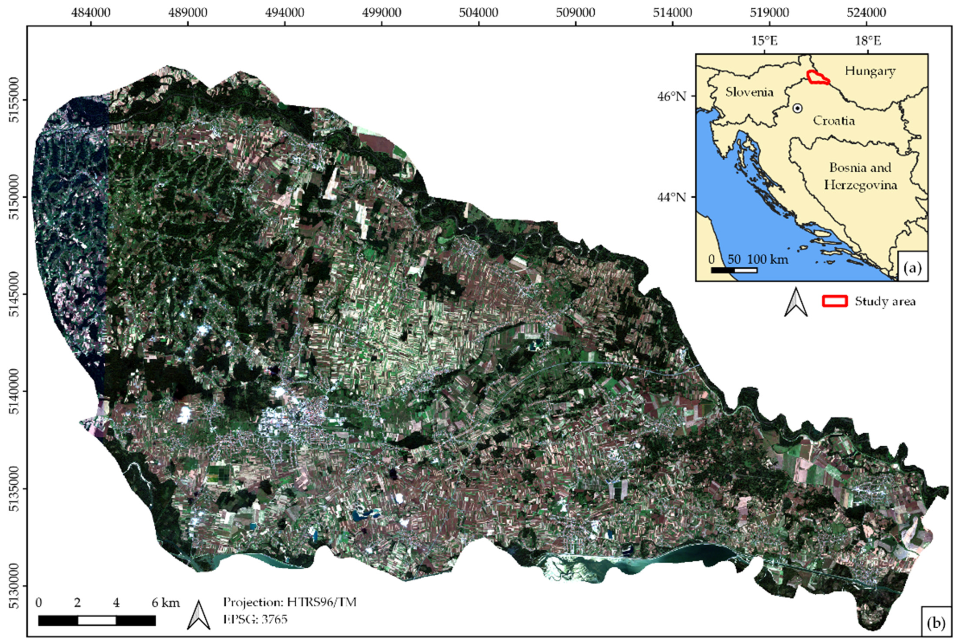
2. Study Area and Datasets

2.1. Study Area

The Međimurje County, illustrated in Figure 1, is one of the main crop product regions and is the northernmost part of Croatia. The study area covers over 700 km2, from which around 360 km2 are used in agriculture, which mostly includes fields of cereals, maize, potato, orchards, and vineyards. According to the Koppen–Geiger climate classification system [35], this region has a temperate oceanic climate (Cfb), characterized by warm summer. The mean annual temperature for 2018 in the study area is 10.2 °C with precipitation of 846 mm/year [36].

2.2. Satellite Datasets

For vegetation mapping in heterogeneous land-cover (LC) areas, multitemporal (MT) satellite imagery is used to characterize phenological changes in vegetation LC classes, instead of using single-date imagery [19]. Therefore, SAR and optical satellite imagery from each temperate season have been used in this research. The SAR data are described in Section 2.2.1; the optical satellite imagery is elaborated in Section 2.2.2; ancillary features derived from SAR and optical imagery are introduced in Section 2.2.3, and topographic data used in different classification scenarios is described in Section 2.2.4.

2.2.1. Sentinel-1 Data

Sentinel-1 (S1) Ground Range Detected (GRD) products in dual-polarization mode (VV + VH) were used in this research (Table 1). Data were downloaded from the European Space Agency (ESA) Data Hub and, as a GRD product, imagery has already been detected, multi-looked, and projected to ground range using an Earth ellipsoid model [37]. Additionally, in ESA SNAP software, data were calibrated to sigma naught (σ0) backscatter intensities, speckle filtered using Lee filter [38], and terrain-correction was made using the shuttle radar topography mission (SRTM) one-arcsecond tiles.

2.2.2. Sentinel-2 Data

The Sentinel-2 (S2) constellation includes two identical satellites (S2A and S2B), which carry a multispectral instrument (MSI) for the acquisition of optical imagery at high spatial resolution (i.e., four spectral bands at 10 m, six bands at 20 m, and three bands at 60 m resolution). The S2 sensor acquired optical imagery during the same periods as S1 (Table 1), and the cloud-free tiles were downloaded in Level-2A (L2A), which provides orthorectified Bottom-Of-Atmosphere (BOA) reflectance, with sub-pixel multispectral registration. For this research, bands with 60 m spatial resolution were not considered due to their sensitivity to aerosol and clouds, whereas 20 m spectral bands were resampled to 10 m using the nearest neighbor method to preserve the pixels’ original values [39].

2.2.3. SAR Texture Features and Multispectral Indices

Since radar backscatter is strongly influenced by the roughness, geometric shape, and dielectric properties of the observed target, radar-derived texture information represents valuable information for classification tasks. Introduced by Haralick et al. [40], grey-level co-occurrence matrix (GLCM), depending on a given direction and a certain distance in the image, estimates the local patterns in image pixel intensities and spatial arrangement. Among many developed texture measures for vegetation mapping, GLCM, combined with the original radar image, is one of the most trustworthy methods for improving mapping accuracy. In this research, a set of nine texture features, derived from the GLCM, were calculated in the SNAP 8.0 software and used for vegetation mapping: Angular Second Moment (ASM), Contrast, Correlation, Dissimilarity, Energy, Entropy, Homogeneity, Mean, and Variance.
Satellite-based indices are commonly calculated from the spectral reflectance of two or more bands [41]. Using these indices indicates the relative abundance of features of interest, such as canopy chlorophyll content estimations, vegetation cover, and leaf area (Normalized Difference Vegetation Index—NDVI; Enhanced Vegetation Index—EVI; Soil Adjusted Vegetation Index—SAVI; Pigment Specific Simple Ratio—PSSRa) or water surfaces (Normalized Difference Water Index—NDWI). Moreover, modified and refined versions of the aforementioned indices were used (Modified Chlorophyll Absorption in Reflectance—MCARI; Green Normalized Vegetation Index—GNDVI; Modified Soil Adjusted Vegetation Index—MSAVI), as well as indices that use narrower red edge bands from S2 (Normalized Difference Index 45—NDI45; Inverted Red-Edge Chlorophyll Index—IRECI). Table 2 shows the multispectral indices employed in this research.

2.2.4. Topographic Data

Some research indicated that using topographic variable data, such as the digital elevation model (DEM) produces major classification enhancements [32,53]. Therefore, shuttle radar topography mission (SRTM) one-arcsecond DEM tiles were resampled to a 10-m spatial resolution by the bilinear interpolation. Additionally, during the test phase of the research, slope and aspect were derived from the SRTM DEM, but their presence as input features brought noise in the dataset, which led to lower classification accuracy. Therefore, the aforementioned features (i.e., slope and aspect) were not further considered as input features for vegetation mapping.

2.3. Reference Data

To reflect the major land-cover classes that are present in the area, reference data were derived, based on our expert knowledge and information, from CORINE, LUCAS, and LPIS land-cover database. Since reference data in the aforementioned databases vary in spatial and semantic consistency, a hybrid classification scheme was devised for this research. Therefore, higher thematic levels from CORINE, LUCAS, and LPIS database were visually interpreted from a time-series of Landsat and Google Earth high-resolution imagery and reduced to the following eight major land-cover classes which were sampled in the study area: cropland, forest, water, built-up, bare soil, grassland, orchard, and vineyard (Table 3). Training and validation pixels were selected at random from the polygon-eroded CORINE and LPIS land-cover maps, and a maximum pixel threshold of 300 pixels per class was set. Afterwards, signatures of the proposed hybrid land-cover classes were checked with LUCAS sample points and visually confirmed from a time-series of high-resolution imagery. This threshold was set following the recommendation from Jensen and Lulla [54] that a number of training pixels should be 10 times the number of the variable used in the classification model. This hybrid approach was proposed in this research, in order to ensure the reproducibility and optimal number of LC classed were chosen since the difference in the number of distinct classes can affect the classification accuracy [55].

3. Methods

The analysis of potentially separable LC classes was conducted using the time-series of optical NDVI values and radar polarization bands. A total of seven cloud-free scenes of the S2 L2A were used to calculate NDVI profiles to identify areas containing different vegetation and agriculture characteristics [56].

3.1. Jeffries–Matusita (JM) Distance

To evaluate the spectral similarity between the LC classes in the reference dataset used for this research, Jeffries–Matusita (JM) distance was calculated [57,58]. This spectral separability measure compares distances between the distribution of classes (e.g., A1 and A2), which are then ranked according to this distance, following the equation:
J M A 1 A 2 = 2 * ( 1 e B )
where B represents the Bhattacharyya distance [56]:
B A 1 A 2 = 1 8 ( m ¯ A 1 m ¯ A 2 ) 2 2 S A 1 2 + S A 2 2 + 1 2 ln [ S A 1 2 + S A 2 2 2 S A 1 + S A 2 ]
where m ¯ A i are average values of LC classes A1 and A2, and S A i are their covariance matrices.

3.2. Random Forest (RF) Classification

For this research, RF classifier was chosen due to the simple parametrization, feature importance estimation in the classification, and short calculation time [3]. Therefore, optimization of the RF hyperparameters and feature importance estimation as input for vegetation mapping will be explained in Section 3.2.1 and Section 3.2.2, respectively.

3.2.1. Hyperparameter Tuning

RF consists of several hyperparameters, which allow users to control the structure and size of the forest (ntree) and its randomness (e.g., number of random variables used in each tree—mtry). Default values for the ntree and mtry parameters are 500 and the square root of the number of input variables, respectively. Therefore, a grid search approach with cross-validation was used in this research for hyperparameter tuning, and optimal parameter values were determined as those that produced the highest classification accuracy.

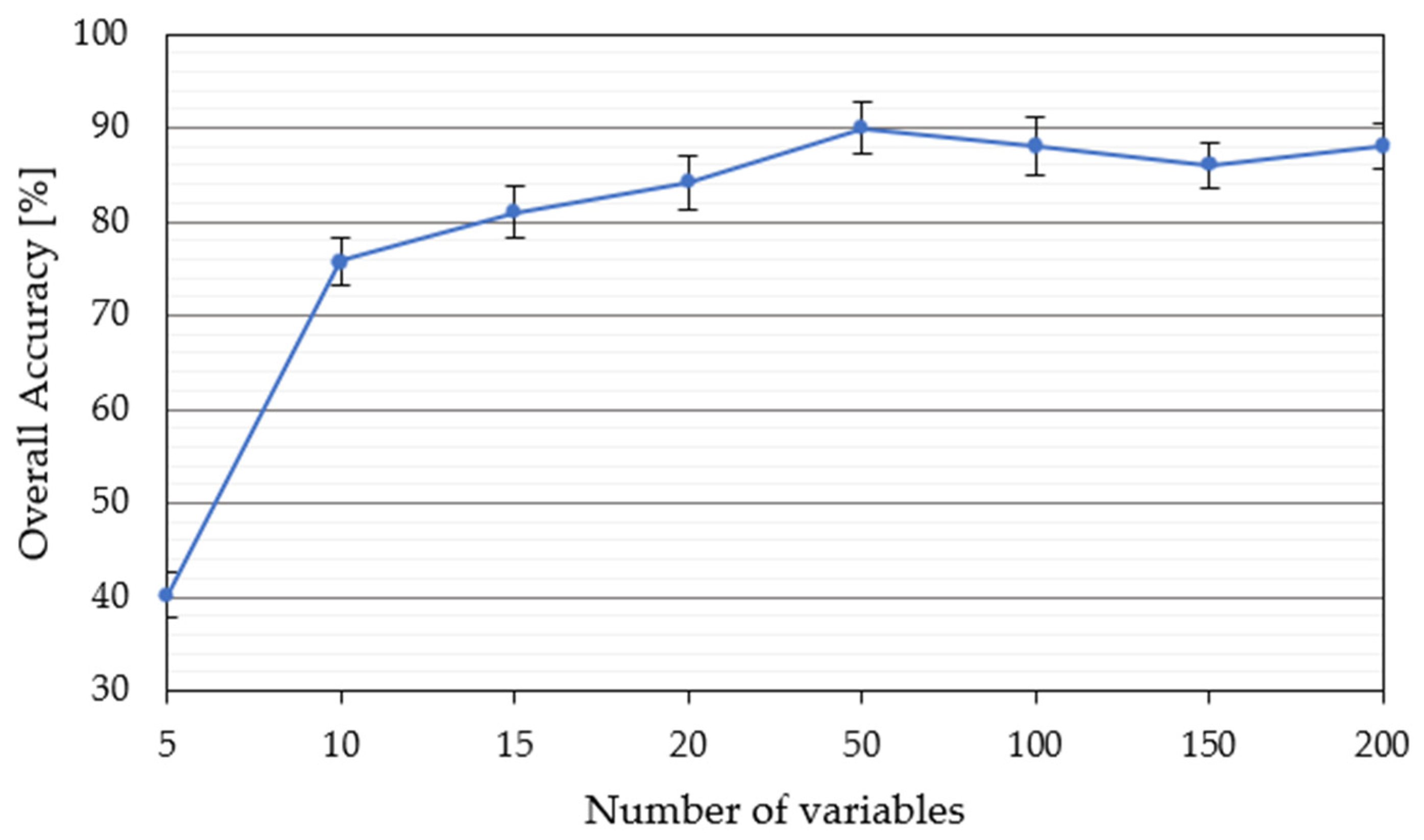
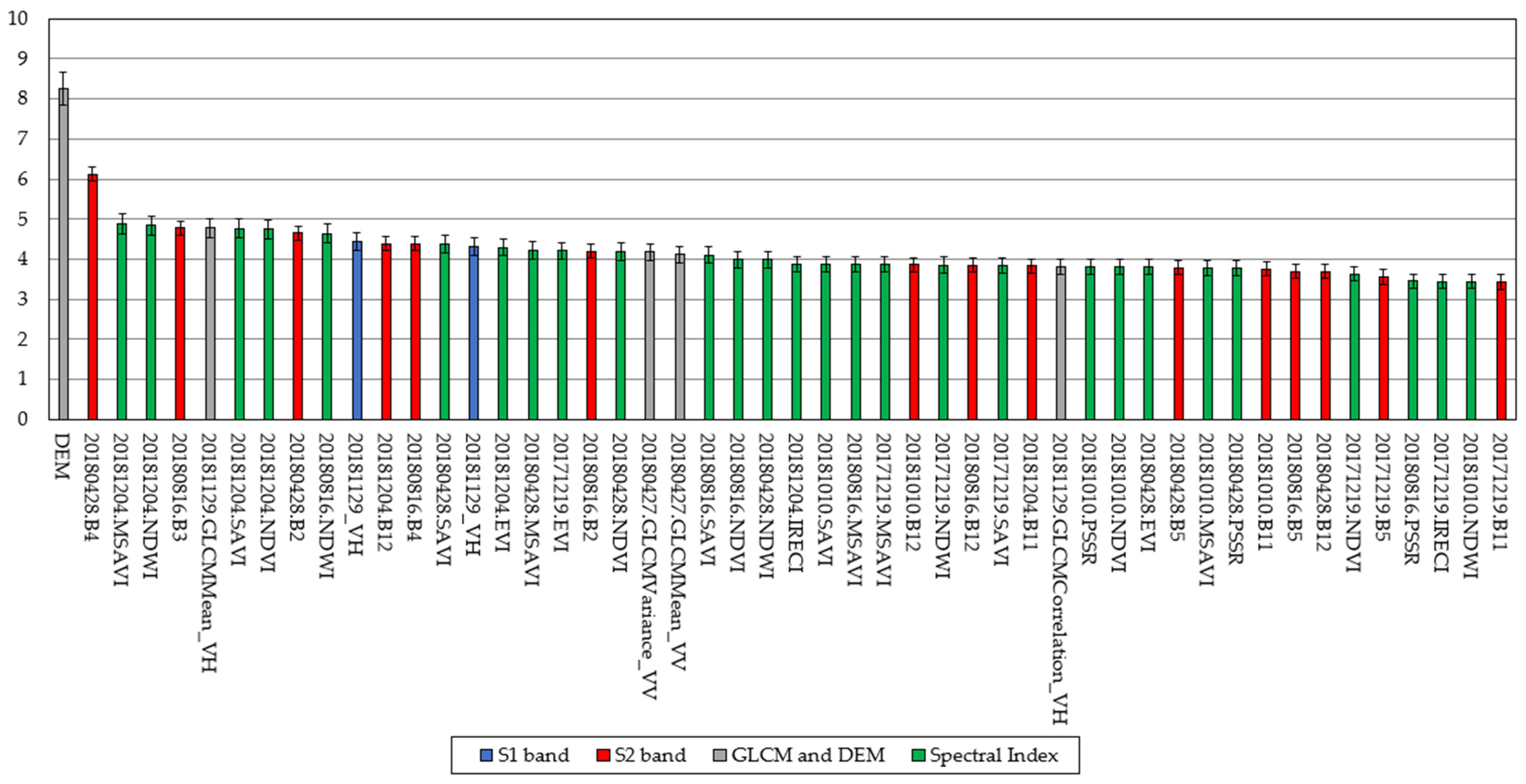
3.2.2. Feature Importance and Selection

During the training phase, RF classifier constructs a bootstrap sample from 2/3 samples of the training dataset, whereas the remaining samples, which are not included in the training subset, are used for internal error estimation called out-of-bag (OOB) error [59]. The random sampling procedure was repeated ten times, allowing to compute average performances with confidence intervals. Afterwards, by evaluating the OOB error of each decision tree when the values of the feature are randomly permuted, the relative importance of each feature can be evaluated [60]. In such a way, mean decrease in accuracy (MDA) can be expressed as [24]:
M D A j = 1 n t = 1 n ( M P t j M t j )
where n is equal to ntree, and Mtj and MPtj denote the OOB error of tree t before and after permuting the values of predictor variable Xj, respectively [61]. MDA value of zero indicates that there is no connection between the predictor and the response feature, whereas the larger positive of MDA value, the more important the feature is for the classification.
Another measure for calculating the feature importance is based on the mean decrease in Gini (MDG), which measures the impurity at each tree node split of a predictor feature, normalized by the number of trees. Similar to MDA, the higher the MDG, the more important the feature is. Similar research in the remote sensing community is not united on which measure to use for feature selection using RG in classification tasks. Belgiu and Dragut [62] reported that most studies in their review used MDA, whereas Cánovas-García and Alonso-Sarría [60] obtained the highest accuracy for all of the classification algorithms using MDG. Since former research used pixel-based and latter object-based classification, MDA was used as a measure for feature selection in this research.

3.3. Accuracy Assessment

The ability to discriminate LC classes was first assessed using optical NDVI profiles and radar backscatter (i.e., VV and VH) coefficients and JM distance, which measures statistical separability between two distributions.
Afterwards, the validation protocol of different classification scenarios used a stratified random sample of 70% of the reference pixels for training and 30% for the validation [33]. Mean overall accuracy (OA) with confidence intervals was reported in this research since twenty random splits of training and validation data were performed [11]. Besides OA, two simple measures (i.e., quantity disagreement (QD) and allocation disagreement (AD) [63]) were used in this research. As reported in the paper by Stehman and Foody [64], Kappa coefficient is highly correlated with OA, and therefore, we opted for QD and AD. The former measure refers to a difference in a number of pixels of the same class and the latter measure refers to a spatial location mismatch for every LC class between the training and test dataset [65]. Additionally, the user’s accuracy (UA), as a measure of the reliability of the map, and producer’s accuracy (PA), as a measure of how well the reference pixels were classified, were computed for individual LC classes [66].
In this research, various classification scenarios (package “randomForest” [67]) and accuracy assessments (package ‘caret’ [68]) were conducted using the R programming language, version 4.0.3., through RStudio version 1.3.1093.

4. Results and Discussion

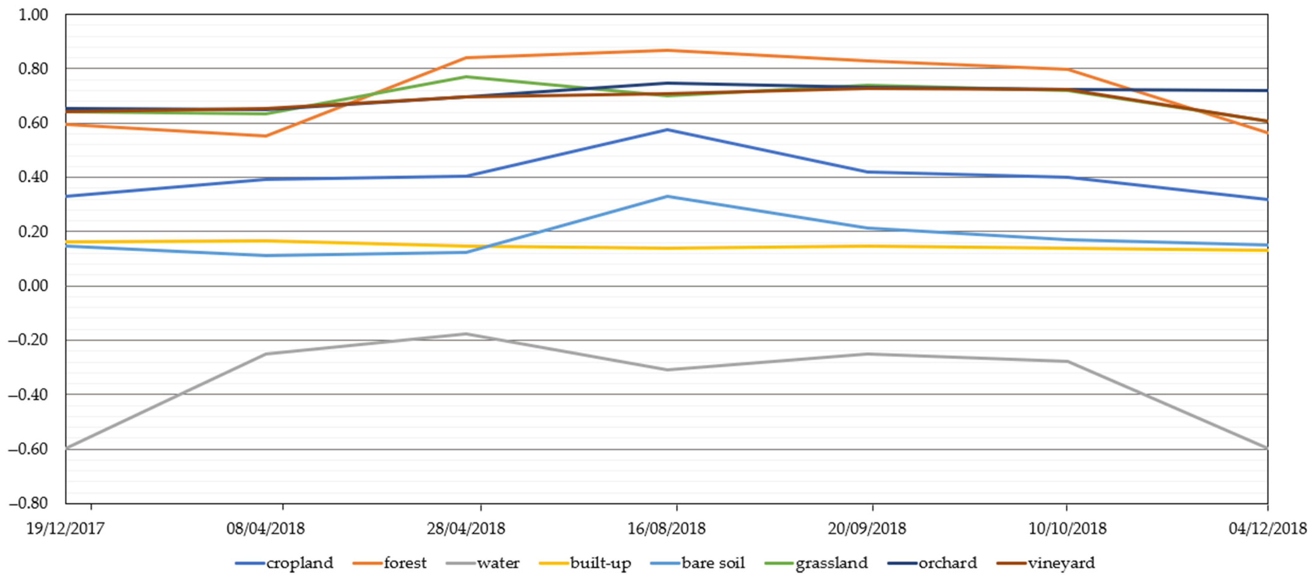
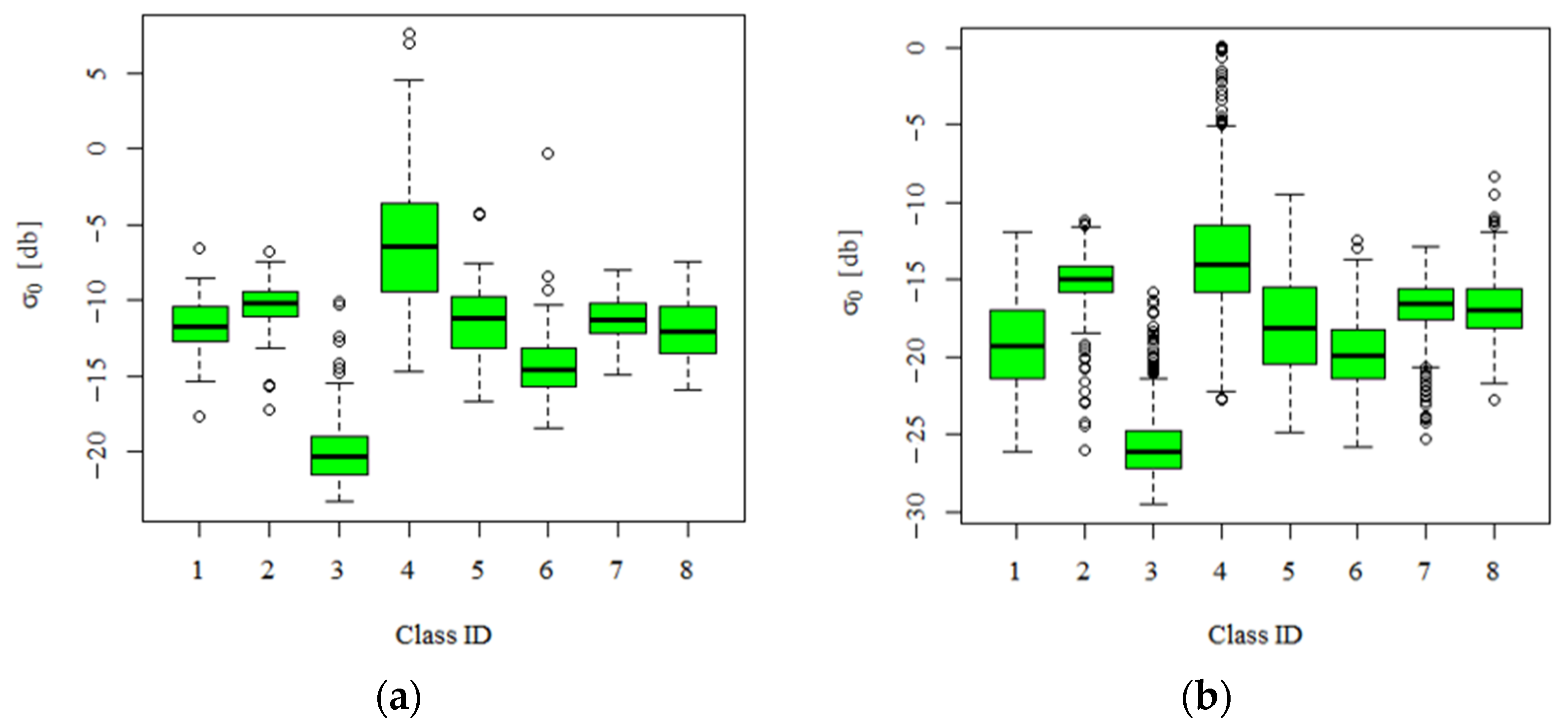
4.1. Optical NDVI and Radar Backscatter (VV, VH) Time-Series

As shown in Figure 2, water and forest can easily be detected throughout the whole season, whereas built-up and bare soil class show a similar pattern, except in August, which can easily be resolved by using additional spectral indices (e.g., SAVI, normalized difference built-up index (NDBI) [69]). Since the cropland class in the investigated study area is consisted mostly of single cropping plant systems (e.g., cereals, maize, and potato), characteristic crop phenology pattern can be recognized, which consists of the sowing (March), growth (from April to August), and harvest (September). The biggest inter-class overlap for separating the vegetation occurs between grassland, orchard, and vineyard. Therefore, in this research, Jeffries–Matusita (JM) distance was used as a spectral separability measure [10,70].
Since the backscatter signal is affected by soil moisture, surface roughness, and terrain topography, the VV and VH polarization bands analysis is presented in Figure 3. Overall, the lowest VV and VH values have water class, since only a very small proportion of backscatter is returned to the sensor due to the side-looking geometry [71]. On the other hand, the highest mean VV and VH values consist of the built-up class, due to the double-bounce effect in the urban areas [72]. Vegetation classes tend to overlap within the VV and VH bands due to the volume scattering, whereas the backscatter values are higher in the VV than VH due to a combination of single bounce (e.g., leaves, stems) and bare soil double-bounce backscatter [73].

4.2. Jeffries–Matusita (JM) Distance Variability Results of Each Class

The JM distance results for the similarity of each class and each sensor calculated are shown in Table 4. For both sensors used in this research (i.e., S1 and S2), the water class was the only LC class identified with JM values above 1.7, which indicates good separability with other classes. This class separability was also confirmed with calculated NDVI profiles (Figure 2). Furthermore, fairly good separation can be found for the forest class using the S1 polarization bands, whereas bare soil class separability is noticeable for the S2 bands. Similar to the NDVI profiles and radar backscatter (VV, VH) values, vegetation classes yielded low JM distance values, indicating that additional features (e.g., spectral indices, GLCM textures) should be used for better class differentiation.
Since this research used reference data from higher thematic levels of CORINE, LUCAS, and LPIS database, the aforementioned eight LC classes were used for different classification scenarios and comparison with similar research. According to Dabboor et al. [74], the JM distance measure is wide in the case of high-dimensional feature space, mostly when hyperspectral imagery is used. In this research, different texture measures were used for increasing the class separability, as noted in the research by Klein et al. [75].

4.3. Random Forest Hyperparameter Tuning Results

For optimization of the RF hyperparameters, a grid search approach with k-fold cross-validation was performed (Table 5), and k was set to 5. Although Cánovas-García and Alonso-Sarría [57] mentioned that RF is not very sensitive to its hyperparameters, ntree and mtry values were set to 1000 and a one half of the input variables for each classification scenario, respectively. A larger number of trees of the forest led to a more stable classification, albeit it can increase computational time for vegetation mapping at regional to global scales.

4.4. Importance and Selection of S1 and S2 Input Features for Vegetation Mapping

Before any classification scenario was conducted, the feature selection was performed for SAR (i.e., S1) and optical (i.e., S2) time-series data, as well as their ancillary features. As shown in Figure 4, major improvements in the overall accuracy are perceptible up to 50 features. An increase from the aforementioned number of features in the classification model provides a negligible improvement in the OA in relation to the computational cost and processing requirements. Therefore, one-fourth most important features from the overall number of input features available for each classification scenario were used in this research.
According to the feature importance approach described in Section 3.2.2, Figure 5 shows the 50 first features sorted by the decreasing MDA. Color coding was used, depending on the source of the input feature (e.g., S1 or S2 band, derived ancillary features from S1 and S2). The digital elevation model (DEM) was the most important input feature for the classification, followed by the summer B4 (i.e., Red) S2 band, and winter MSAVI and NDWI S2 indices. Overall, for S1, the VH polarization band was the most important feature among the first 50 features, whereas GLCM Mean, Variance, and Correlation were the most important features among the nine textural features used in this research. The former variable (i.e., VH) is expected to be included in the final classification model, since it contains volume scattering information [76], whereas the latter GLCM features have already been proven for vegetation mapping [20,41].
In terms of S2, B12, B11, and B5 (i.e., SWIR2, SWIR1, and RE1) are the most present S2 spectral bands. These results coincide with similar research [77], e.g., Abdi [78] where nearly half of the input S2 variables belonged to the RE and SWIR bands, included in scenes from spring and summer dates. The high importance of the RE1 band could be associated with the mapping of different crop types [79], whereas SWIR bands were found to be important for mapping the forest class [80]. In the research by Immitzer et al. [81], the aforementioned S2 bands were most important for tree species and crop type mapping using single-date S2 imagery. In this research, the spectral indices were represented the most, with 28 of them among the 50 input features. NDVI, NDWI, SAVI, and MSAVI were represented the most in the classification model within this feature group, whereas NDI45, MCARI, and GNDVI were not included at all in the model. This is expected, since vegetation phenology in the time-series can be greatly represented with NDVI [82], and other indices provided good separation between other LC classes. In terms of the relevance of time periods, the spring dates are the most present for features that are connected with the vegetation classes, whereas December appeared to be the most important month for discriminating other non-vegetation LC classes.
The aforementioned feature selection results coincide with similar research. Jin et al. [19] evaluated the variable importance of Landsat imagery through MDA and Gini index using RF for LC classification. Summer NDVI and NIR band, DEM, GLCM mean, and contrast were the key input features for classification, which achieved OA of 88.9%. Abdi [78] classified boreal landscape using S2 imagery and RF, support vector machine (SVM), extreme gradient boosting (XGB), and deep learning (DL) classifiers. RE and SWIR S2 bands were the most important features, and interestingly, none of the spectral indices were ranked highly in his research, probably because of the high correlation with the red edge bands. RF achieved an overall accuracy of 73.9%. Tavares et al. [77] used S1 and S2 data for urban area classification. Red and SWIR S2 bands were identified as the most significant contributors to the classification, whereas VV and GLCM mean were the most important features from S1 and texture features, respectively. The authors agree that DEM should be included for major classification enhancements, which was done in our research. The integration of S1 and S2 data yielded the highest OA of 91.07% [74].

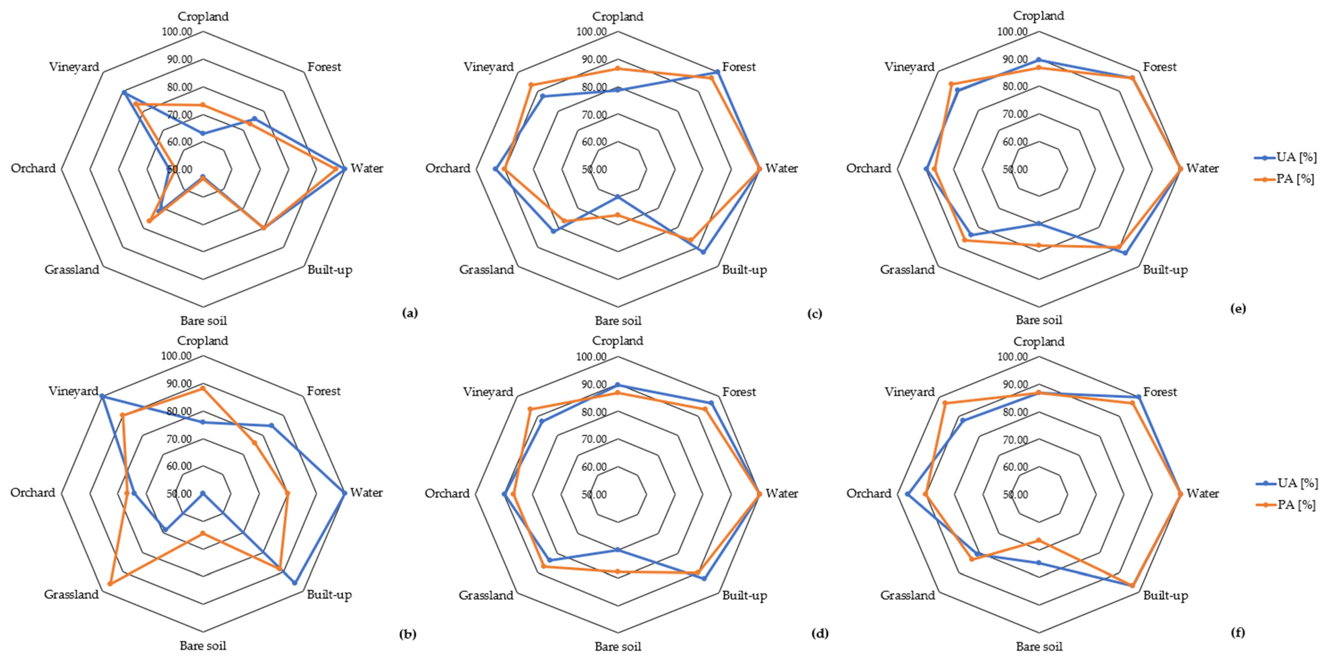
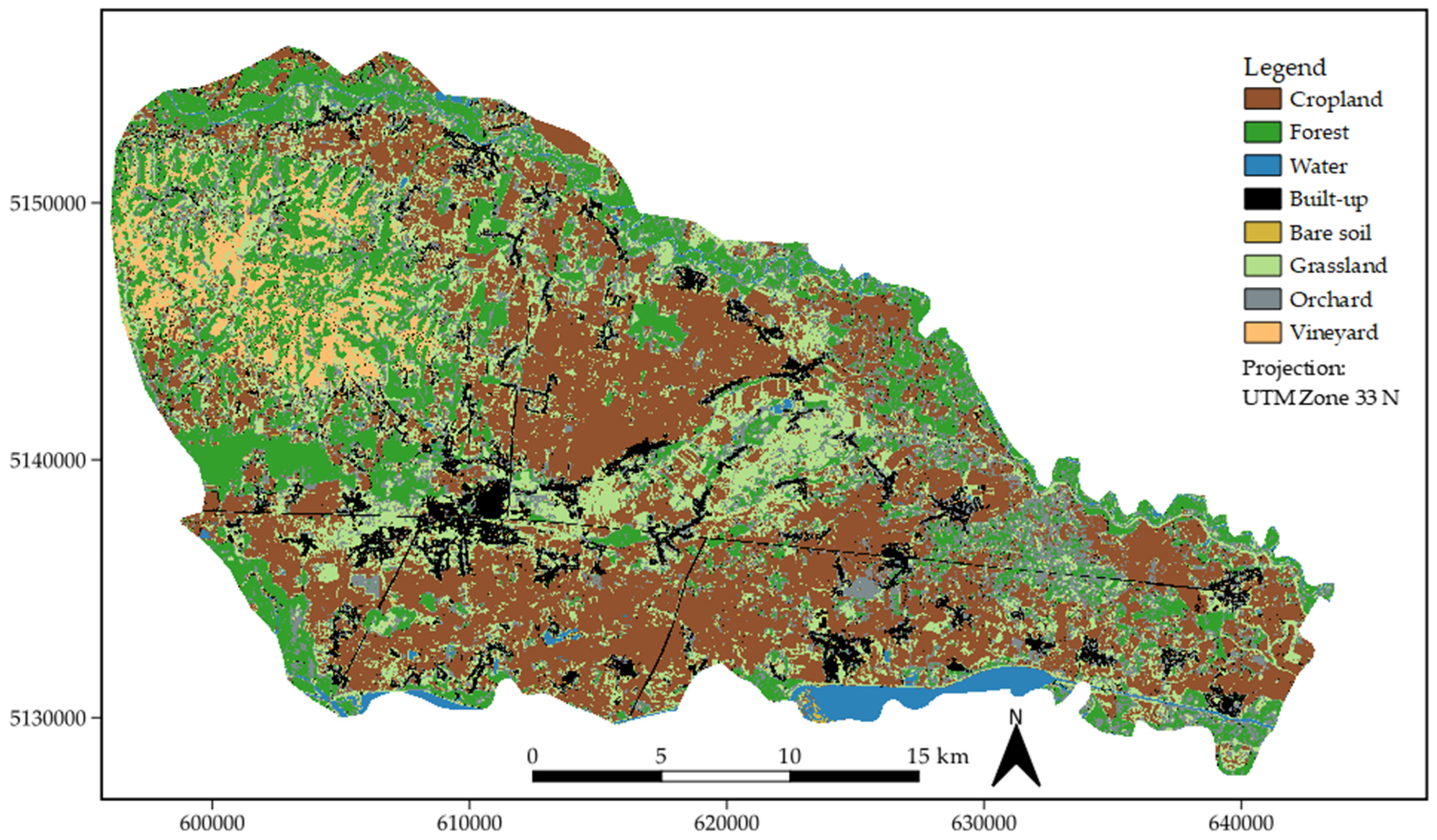
4.5. Accuracy Assessment

Confusion or error matrix [83] was computed for six different classification scenarios in a time-series (i.e., S1 and S2 alone, S1 with GLCM, S2 with Indices, S1 and S2, and all features together). Overall accuracy (OA), quantity disagreement (QD), and allocation disagreement (AD) were derived from the confusion matrix (Section 3.3).
Table 6 shows that the highest OA of 91.78% was achieved using combined S1 with S2 features, whereas classification using only S1 bands yielded the lowest OA of 79.45%. Interestingly, classification using all available features achieved lower OA than S1 with S2, leading to a conclusion that ancillary S1 and S2 features (i.e., GLCM and spectral indices) brought additional noise in the data, leading to a decrease in the classification. On the other hand, QD was lower for classification using all features compared to S1 with S2 classification, which means that the level of difference in the number of pixels between the reference map versus the classified map is different for the classification using all features, but the number of misallocated pixels is higher (i.e., more pixels are omitted from a particular LC class). The addition of texture features (i.e., GLCM) for S1 and spectral indices for S2 yielded an increase of 2.26% and 1.33% of OA, respectively. Similar results were obtained in the research from Sun et al. [84], where the RF classifier provided the best crop-type mapping results. Classification using S1 and S2 sensors yielded OA of 92%, whereas the index features were most dominant in the classification results.
To assess the ability of differentiation between the LC classes, UA and PA values for each classification scenario is presented in Figure 6. As indicated in Table 6, classification using S1 features only poorly predicted LC classes, except for the water class (Figure 6a), which achieved very high UA values in each scenario, irrespective of the sensor used. As seen in Figure 6b, GLCM features improved the classification accuracy in vegetation classes, and similar to [85], texture features improved the supervised classification for urban areas. Although S2 and S2 with Indices (Figure 6c,d, respectively) produced similar results in this research, cropland and bare soil classes were better differentiated when the spectral indices were used. Therefore, it is confirmed that for vegetation mapping, when enough optical imagery is available for the time-series analysis, it outperforms LC classifications solely using SAR data in many agricultural applications. In order to mitigate this obstacle, Holtgrave et al. [86] compared S1 and S2 data and indices for agricultural monitoring. In their study, radar vegetation index (RVI) and VH backscatter had the strongest correlation with the spectral indices, whereas the soil more influences VV backscatter in general. Therefore, SAR indices need to be investigated for vegetation mapping in future research.
For the best classification scenario (i.e., S1 with S2), forest and water class achieved the highest UA values to measure map reliability. From other vegetation LC classes, UA was highest for orchard, whereas PA was highest for the vineyard. Cropland was mostly committed to the bare soil or orchard class, while bare soil was the most underestimated LC class (i.e., high omission error) due to the confusion with the built-up class. In order to reduce the misclassification between built-up and bare soil class, built-up indices, such as normalized difference built-up index (NDBI), built-up index (BUI), built-up area extraction index (BAEI), etc., should be included in the classification [38]. Similar to our research, Jin et al. [19] yielded UA higher than 90% for vegetation classes, and the confusion of grassland, forest, and cropland could be associated with their accuracy errors. Sonobe et al. [10] investigated the potential of SAR (i.e., S1) and optical (i.e., S2) data for crop classification. Accuracy metrics for RF classifier were 95.70%, 2.83%, and 1.47%, in terms of OA, AD, and QD, respectively. Most of the misclassified fields were below 200 a, mostly for the grassland and maize class. Overall, the large potential of S1 and S2 data was proven for crop mapping, mostly of their high temporal resolution and free of charge availability.
Figure 7 represents the best supervised pixel-based classification scenario (i.e., S1 with S2) using a RF classifier. Water and forest were in good agreement with testing data, whereas some bare soil pixels were classified as cropland or orchard. Having added S2 imagery extracted the urban area more accurately, including main traffic roads. The confusion of orchards, cropland, and bare soil was the main cause of their misclassification errors. Vineyards are located in the northwestern part of the study areas and are mostly situated on the slopes of hills. Due to the large terrain slopes or SAR shadowing [87], it can be seen in Figure 7 that some confusion between built-up and vineyards occurred. This effect can be removed with the help of high-quality DEM or GLCM textural features [88].

4.6. Impact of the Reference Dataset on Classification Accuracies

This research used a hybrid reference dataset derived from CORINE, LUCAS, and LPIS land-cover datasets, which collect in situ data every six, three, and one year, respectively. The goal of the hybrid dataset was to take the best of each representation, where only an agreement is targeted [89]. As noted in the research by Baudoux et al. [28], within this approach, two main limitations can arise—spatial [31] and semantic consistency [90]. A former limitation was solved using a GRID location of the LUCAS sample points since a difference between GRID and GPS locations exists [31]. Since the nomenclatures across different LC databases are not standardized, the latter limitation was resolved using n- > 1 associations between each class of each nomenclature (as described in Section 2.3), which resulted in identifying eight major LC classes. This proved to be a good trade-off between the overall classification accuracy and the spectral difference between the LC classes since through an analysis of 64 similar research, Van Thinh et al. [91] noted that a significant decrease in OA occurs when increasing the number of classes. Moreover, variations in the performance of the RF classifier, in terms of OA, could occur due to the imbalanced and mislabeled training datasets. The former obstacle could be mitigated using a weighted confusion matrix, which provides confidence estimates associated with correctly and misclassified instances in the RF classification model [92], whereas the latter obstacle is little influenced for low random noise levels up to 25%–30% [93]. This research used a balanced training dataset, which, as presented in [92], resulted in the lowest overall error rates for classification scenarios.
In this research, S1 and S2 imagery along with RF classifier were used for vegetation mapping on a proposed hybrid reference dataset. Compared to similar research, Dabija et al. [94] compared SVM and RF for 14 CORINE classes using multitemporal S2 and Landsat 8 imagery. SVM with radial kernel yielded the highest OA, whereas RF achieved OA of 80%. Close et al. [95] used S2 imagery and the LUCAS reference dataset for LC mapping in Belgium. Single-date and multitemporal classifications of five LC classes were tested for different seasons, and RF yielded an OA of 88%. In their research, the size of the training samples was also investigated, and the highest OA was achieved with approximately 400 sample points of a balanced training dataset. Balzter et al. [32] used S1 imagery and RF classifier for mapping CORINE land cover. Additional texture features were derived from S1 imagery, and in addition, SRTM was used as an input feature for landscape topography. Hybrid CORINE Level 2/3 classification scheme was proposed in the research, which reduced 44 LC classes to 27. The highest classification result, in terms of OA, of 68.4% was achieved using S1, texture bands, and DEM data. As noted in the review paper by Phiri et al. [96], RF and SVM classifiers provide the highest accuracies in the range from 89% to 92% for land cover/use mapping using S2 imagery, which was confirmed in our research.

5. Conclusions

This research aimed to evaluate the classification accuracy of multi-source time-series data (i.e., radar and optical imagery) with a high temporal and spatial resolution for vegetation mapping.
Sentinel-1 SAR time-series were combined with Sentinel-2 imagery showing that an improvement in classification accuracy can be obtained in regard to the results with each sensor independently. In this research, Random Forest was used as a classifier for vegetation mapping, due to the ability to deal with high-dimensional data through feature importance strategy. The aforementioned measure allowed us to use one-fourth of input variables as a trade-off between model complexity and overall accuracy. Therefore, in this research, the highest OA of 91.78% was achieved using S1 with S2, with a total disagreement of 8.22%.
For vegetation mapping, the most pertinent features derived from S1 imagery were GLCM Mean and Variance, along with the VH polarization band. Considering the spectral indices derived from S2 imagery, NDVI, NDWI, SAVI, and MSAVI contained most of the information needed for vegetation mapping, along with Red and SWIR S2 spectral bands. Overall, SRTM DEM produced major classification enhancement as an input feature for vegetation mapping.
Within this research, a hybrid classification scheme was derived from European (i.e., LUCAS and CORINE) and national (LPIS) land-cover (LC) databases. The results of this study demonstrated that the aforementioned approach is well-suited for vegetation mapping using Sentinel imagery, which can be applied for large-scale LC classifications.
Future research should focus on more advanced deep learning techniques (e.g., convolutional neural networks), which can exploit relations between pixels and objects on the image. Furthermore, these deep learning methods need many training samples, which can be derived from the proposed hybrid classification scheme and combined with S1 and S2 time-series imagery.

Author Contributions

Conceptualization, D.D. and M.G.; methodology, M.G.; software, D.D.; validation, M.G., D.D., and D.M.; formal analysis, D.D. and M.G.; investigation, D.D.; resources, M.G. and D.M.; data curation, D.D. and M.G.; writing—original draft preparation, D.D. and M.G.; writing—review and editing, D.D., M.G, and D.M.; visualization, D.D. and M.G.; supervision, M.G. and D.M.; project administration, D.M.; funding acquisition, M.G. and D.M. All authors have read and agreed to the published version of the manuscript.

Funding

This research was funded by the Croatian Science Foundation for the GEMINI project: “Geospatial Monitoring of Green Infrastructure by Means of Terrestrial, Airborne and Satellite Imagery” (Grant No. HRZZIP-2016-06-5621); and by the University of Zagreb for the project: “Advanced photogrammetry and remote sensing methods for environmental change monitoring” (Grant No. RS4ENVIRO).

Institutional Review Board Statement

Not applicable.

Informed Consent Statement

Not applicable.

Data Availability Statement

All data are publicly available online: S1 and S2 imagery were acquired from the Copernicus Open Access Hub (https://scihub.copernicus.eu, accessed on 8 January 2021), Corine Land Cover data from Copernicus Land Monitoring Service (https://land.copernicus.eu/pan-european/corine-land-cover/clc2018, accessed on 8 January 2021), Land Use and Coverage Area Frame Survey (LUCAS) data from Copernicus Land Monitoring Service (https://land.copernicus.eu/imagery-in-situ/lucas/lucas-2018, accessed on 17 March 2021), Land Parcel Identification System (LPIS) data from National Spatial Data Infrastructure (https://registri.nipp.hr/izvori/view.php?id=401, accessed on 17 March 2021).

Conflicts of Interest

The authors declare no conflict of interest.

References

  1. Gong, P.; Wang, J.; Yu, L.; Zhao, Y.; Zhao, Y.; Liang, L.; Niu, Z.; Huang, X.; Fu, H.; Liu, S.; et al. Finer Resolution Observation and Monitoring of Global Land Cover: First Mapping Results with Landsat TM and ETM+ Data. Int. J. Remote Sens. 2013, 34, 2607–2654. [Google Scholar] [CrossRef] [Green Version]
  2. Liu, X.; Liang, X.; Li, X.; Xu, X.; Ou, J.; Chen, Y.; Li, S.; Wang, S.; Pei, F. A Future Land Use Simulation Model (FLUS) for Simulating Multiple Land Use Scenarios by Coupling Human and Natural Effects. Landsc. Urban Plan. 2017, 168, 94–116. [Google Scholar] [CrossRef]
  3. Mercier, A.; Betbeder, J.; Rumiano, F.; Baudry, J.; Gond, V.; Blanc, L.; Bourgoin, C.; Cornu, G.; Ciudad, C.; Marchamalo, M.; et al. Evaluation of Sentinel-1 and 2 Time Series for Land Cover Classification of Forest–Agriculture Mosaics in Temperate and Tropical Landscapes. Remote Sens. 2019, 11, 979. [Google Scholar] [CrossRef] [Green Version]
  4. Dobrinić, D.; Medak, D.; Gašparović, M. Integration Of Multitemporal Sentinel-1 And Sentinel-2 Imagery For Land-Cover Classification Using Machine Learning Methods. Int. Arch. Photogramm. Remote Sens. Spat. Inf. Sci. 2020, 43, 91–98. [Google Scholar] [CrossRef]
  5. Zhang, X.; Friedl, M.A.; Schaaf, C.B.; Strahler, A.H.; Hodges, J.C.F.; Gao, F.; Reed, B.C.; Huete, A. Monitoring Vegetation Phenology Using MODIS. Remote Sens. Environ. 2003, 84, 471–475. [Google Scholar] [CrossRef]
  6. Gao, F.; Hilker, T.; Zhu, X.; Anderson, M.; Masek, J.; Wang, P.; Yang, Y. Fusing Landsat and MODIS Data for Vegetation Monitoring. IEEE Geosci. Remote Sens. Mag. 2015, 3, 47–60. [Google Scholar] [CrossRef]
  7. Schultz, M.; Clevers, J.G.P.W.; Carter, S.; Verbesselt, J.; Avitabile, V.; Quang, H.V.; Herold, M. Performance of Vegetation Indices from Landsat Time Series in Deforestation Monitoring. Int. J. Appl. Earth Obs. Geoinf. 2016, 52, 318–327. [Google Scholar] [CrossRef]
  8. Bhandari, S.; Phinn, S.; Gill, T. Preparing Landsat Image Time Series (LITS) for Monitoring Changes in Vegetation Phenology in Queensland, Australia. Remote Sens. 2012, 4, 1856–1886. [Google Scholar] [CrossRef] [Green Version]
  9. Vuolo, F.; Neuwirth, M.; Immitzer, M.; Atzberger, C.; Ng, W.T. How Much Does Multi-Temporal Sentinel-2 Data Improve Crop Type Classification? Int. J. Appl. Earth Obs. Geoinf. 2018, 72, 122–130. [Google Scholar] [CrossRef]
  10. Sonobe, R.; Yamaya, Y.; Tani, H.; Wang, X.; Kobayashi, N.; Mochizuki, K.-I. Assessing the Suitability of Data from Sentinel-1A and 2A for Crop Classification. GISci. Remote Sens. 2017, 54, 918–938. [Google Scholar] [CrossRef]
  11. Inglada, J.; Vincent, A.; Arias, M.; Marais-Sicre, C. Improved Early Crop Type Identification by Joint Use of High Temporal Resolution Sar and Optical Image Time Series. Remote Sens. 2016, 8, 362. [Google Scholar] [CrossRef] [Green Version]
  12. Gašparović, M.; Klobučar, D. Mapping Floods in Lowland Forest Using Sentinel-1 and Sentinel-2 Data and an Object-Based Approach. Forests 2021, 12, 553. [Google Scholar] [CrossRef]
  13. Tomiyasu, K. Tutorial Review of Synthetic-Aperture Radar (SAR) with Applications to Imaging of the Ocean Surface. Proc. IEEE 1978, 66, 563–583. [Google Scholar] [CrossRef]
  14. Moreira, A.; Prats-iraola, P.; Younis, M.; Krieger, G.; Hajnsek, I.; Papathanassiou, K.P. A tutorial on synthetic aperture radar. IEEE Geosci. Remote Sens. Mag. 2013, 1, 6–43. [Google Scholar] [CrossRef] [Green Version]
  15. Gašparović, M.; Dobrinić, D. Comparative Assessment of Machine Learning Methods for Urban Vegetation Mapping Using Multitemporal Sentinel-1 Imagery. Remote Sens. 2020, 12, 1952. [Google Scholar] [CrossRef]
  16. Chauhan, S.; Darvishzadeh, R.; Lu, Y.; Boschetti, M.; Nelson, A. Understanding Wheat Lodging Using Multi-Temporal Sentinel-1 and Sentinel-2 Data. Remote Sens. Environ. 2020, 243, 111804. [Google Scholar] [CrossRef]
  17. Frantz, D.; Schug, F.; Okujeni, A.; Navacchi, C.; Wagner, W.; van der Linden, S.; Hostert, P. National-Scale Mapping of Building Height Using Sentinel-1 and Sentinel-2 Time Series. Remote Sens. Environ. 2021, 252, 112128. [Google Scholar] [CrossRef]
  18. Zhang, W.; Brandt, M.; Wang, Q.; Prishchepov, A.V.; Tucker, C.J.; Li, Y.; Lyu, H.; Fensholt, R. From Woody Cover to Woody Canopies: How Sentinel-1 and Sentinel-2 Data Advance the Mapping of Woody Plants in Savannas. Remote Sens. Environ. 2019, 234, 111465. [Google Scholar] [CrossRef]
  19. Jin, Y.; Liu, X.; Chen, Y.; Liang, X. Land-Cover Mapping Using Random Forest Classification and Incorporating NDVI Time-Series and Texture: A Case Study of Central Shandong. Int. J. Remote Sens. 2018, 39, 8703–8723. [Google Scholar] [CrossRef]
  20. Gašparović, M.; Dobrinić, D. Green Infrastructure Mapping in Urban Areas Using Sentinel-1 Imagery. Croat. J. For. Eng. 2021, 42, 1–20. [Google Scholar] [CrossRef]
  21. Isaac, E.; Easwarakumar, K.S.; Isaac, J. Urban Landcover Classification from Multispectral Image Data Using Optimized AdaBoosted Random Forests. Remote Sens. Lett. 2017, 8, 350–359. [Google Scholar] [CrossRef]
  22. Feng, Q.; Yang, J.; Zhu, D.; Liu, J.; Guo, H.; Bayartungalag, B.; Li, B. Integrating Multitemporal Sentinel-1/2 Data for Coastal Land Cover Classification Using a Multibranch Convolutional Neural Network: A Case of the Yellow River Delta. Remote Sens. 2019, 11, 1006. [Google Scholar] [CrossRef] [Green Version]
  23. Paris, C.; Weikmann, G.; Bruzzone, L. Monitoring of Agricultural Areas by Using Sentinel 2 Image Time Series and Deep Learning Techniques. Proc. SPIE. 2020, 11533, 115330K. [Google Scholar] [CrossRef]
  24. Han, H.; Guo, X.; Yu, H. Variable Selection Using Mean Decrease Accuracy and Mean Decrease Gini Based on Random Forest. In Proceedings of the 2016 7th IEEE International Conference on Software Engineering and Service Science (ICSESS), Beijing, China, 26–28 August 2016; pp. 219–224. [Google Scholar] [CrossRef]
  25. Saeys, Y.; Inza, I.; Larrañaga, P. A Review of Feature Selection Techniques in Bioinformatics. Bioinformatics 2007, 23, 2507–2517. [Google Scholar] [CrossRef] [PubMed] [Green Version]
  26. Jović, A.; Brkić, K.; Bogunović, N. A Review of Feature Selection Methods with Applications. In Proceedings of the 2015 38th International Convention on Information and Communication Technology, Electronics and Microelectronics, MIPRO 2015-Proceedings, Opatija, Croatia, 25–29 May 2015; pp. 1200–1205. [Google Scholar]
  27. Breiman, L. Random Forests. Mach. Learn. 2001, 45, 5–32. [Google Scholar] [CrossRef] [Green Version]
  28. Baudoux, L.; Inglada, J.; Mallet, C. Toward a Yearly Country-Scale CORINE Land-Cover Map without Using Images: A Map Translation Approach. Remote Sens. 2021, 13, 1060. [Google Scholar] [CrossRef]
  29. Van Tricht, K.; Gobin, A.; Gilliams, S.; Piccard, I. Synergistic Use of Radar Sentinel-1 and Optical Sentinel-2 Imagery for Crop Mapping: A Case Study for Belgium. Remote Sens. 2018, 10, 1642. [Google Scholar] [CrossRef] [Green Version]
  30. Belgiu, M.; Csillik, O. Sentinel-2 Cropland Mapping Using Pixel-Based and Object-Based Time-Weighted Dynamic Time Warping Analysis. Remote Sens. Environ. 2018, 204, 509–523. [Google Scholar] [CrossRef]
  31. Weigand, M.; Staab, J.; Wurm, M.; Taubenböck, H. Spatial and Semantic Effects of LUCAS Samples on Fully Automated Land Use/Land Cover Classification in High-Resolution Sentinel-2 Data. Int. J. Appl. Earth Obs. Geoinf. 2020, 88, 102065. [Google Scholar] [CrossRef]
  32. Balzter, H.; Cole, B.; Thiel, C.; Schmullius, C. Mapping CORINE Land Cover from Sentinel-1A SAR and SRTM Digital Elevation Model Data Using Random Forests. Remote Sens. 2015, 7, 14876–14898. [Google Scholar] [CrossRef] [Green Version]
  33. Olofsson, P.; Foody, G.M.; Herold, M.; Stehman, S.V.; Woodcock, C.E.; Wulder, M.A. Good Practices for Estimating Area and Assessing Accuracy of Land Change. Remote Sens. Environ. 2014, 148, 42–57. [Google Scholar] [CrossRef]
  34. Stehman, S.V. Sampling Designs for Accuracy Assessment of Land Cover. Int. J. Remote Sens. 2009, 30, 5243–5272. [Google Scholar] [CrossRef]
  35. Beck, H.E.; Zimmermann, N.E.; McVicar, T.R.; Vergopolan, N.; Berg, A.; Wood, E.F. Present and Future Köppen-Geiger Climate Classification Maps at 1-Km Resolution. Sci. Data 2018, 5, 1–12. [Google Scholar] [CrossRef] [PubMed] [Green Version]
  36. World Weather Online. Available online: https://www.worldweatheronline.com/cakovec-weather-history/medimurska/hr.aspx (accessed on 15 January 2021).
  37. Torres, R.; Snoeij, P.; Geudtner, D.; Bibby, D.; Davidson, M.; Attema, E.; Potin, P.; Rommen, B.Ö.; Floury, N.; Brown, M.; et al. GMES Sentinel-1 Mission. Remote Sens. Environ. 2012, 120, 9–24. [Google Scholar] [CrossRef]
  38. Lee, J.S. Digital Image Enhancement and Noise Filtering by Use of Local Statistics. IEEE Trans. Pattern Anal. Mach. Intell. 1980, 2, 165–168. [Google Scholar] [CrossRef] [Green Version]
  39. Osgouei, P.E.; Kaya, S.; Sertel, E.; Alganci, U. Separating Built-up Areas from Bare Land in Mediterranean Cities Using Sentinel-2A Imagery. Remote Sens. 2019, 11, 345. [Google Scholar] [CrossRef] [Green Version]
  40. Haralick, R.M.; Shanmugam, K.; Dinstein, I. Textural Features for Image Classification. IEEE Trans. Syst. Man Cybern. 1973, 3, 610–621. [Google Scholar] [CrossRef] [Green Version]
  41. Clerici, N.; Valbuena Calderón, C.A.; Posada, J.M. Fusion of Sentinel-1a and Sentinel-2A Data for Land Cover Mapping: A Case Study in the Lower Magdalena Region, Colombia. J. Maps 2017, 13, 718–726. [Google Scholar] [CrossRef] [Green Version]
  42. Tucker, C.J. Red and Photographic Infrared Linear Combinations for Monitoring Vegetation. Remote Sens. Environ. 1979, 8, 127–150. [Google Scholar] [CrossRef] [Green Version]
  43. McFeeters, S.K. The Use of the Normalized Difference Water Index (NDWI) in the Delineation of Open Water Features. Int. J. Remote Sens. 1996, 17, 1425–1432. [Google Scholar] [CrossRef]
  44. Huete, A.; Didan, K.; Miura, T.; Rodriguez, E.P.; Gao, X.; Ferreira, L.G. Overview of the Radiometric and Biophysical Performance of the MODIS Vegetation Indices. Remote Sens. Environ. 2002, 83, 195–213. [Google Scholar] [CrossRef]
  45. Huete, A.R. A Soil-Adjusted Vegetation Index (SAVI). Remote Sens. Environ. 1988, 25, 295–309. [Google Scholar] [CrossRef]
  46. Delegido, J.; Verrelst, J.; Alonso, L.; Moreno, J. Evaluation of Sentinel-2 Red-Edge Bands for Empirical Estimation of Green LAI and Chlorophyll Content. Sensors 2011, 11, 7063–7081. [Google Scholar] [CrossRef] [Green Version]
  47. Daughtry, C.S.T.; Walthall, C.L.; Kim, M.S.; De Colstoun, E.B.; McMurtrey, J.E. Estimating Corn Leaf Chlorophyll Concentration from Leaf and Canopy Reflectance. Remote Sens. Environ. 2000, 74, 229–239. [Google Scholar] [CrossRef]
  48. Gitelson, A.A.; Merzlyak, M.N. Remote Sensing of Chlorophyll Concentration in Higher Plant Leaves. Adv. Sp. Res. 1998, 22, 689–692. [Google Scholar] [CrossRef]
  49. Qi, J.; Chehbouni, A.; Huete, A.R.; Kerr, Y.H.; Sorooshian, S. A Modified Soil Adjusted Vegetation Index. Remote Sens. Environ. 1994, 48, 119–126. [Google Scholar] [CrossRef]
  50. Blackburn, G.A. Spectral Indices for Estimating Photosynthetic Pigment Concentrations: A Test Using Senescent Tree Leaves. Int. J. Remote Sens. 1998, 19, 657–675. [Google Scholar] [CrossRef]
  51. Frampton, W.J.; Dash, J.; Watmough, G.; Milton, E.J. Evaluating the Capabilities of Sentinel-2 for Quantitative Estimation of Biophysical Variables in Vegetation. ISPRS J. Photogramm. Remote Sens. 2013, 82, 83–92. [Google Scholar] [CrossRef] [Green Version]
  52. Gonzalez-Piqueras, J.; Calera, A.; Gilabert, M.A.; Cuesta, A.; De la Cruz Tercero, F. Estimation of crop coefficients by means of optimized vegetation indices for corn. Remote Sens. Agric. Ecosyst. Hydrol. V 2004, 5232, 110. [Google Scholar] [CrossRef]
  53. Chatziantoniou, A.; Psomiadis, E.; Petropoulos, G. Co-Orbital Sentinel 1 and 2 for LULC Mapping with Emphasis on Wetlands in a Mediterranean Setting Based on Machine Learning. Remote Sens. 2017, 9, 1259. [Google Scholar] [CrossRef] [Green Version]
  54. Jensen, J.R.; Lulla, K. Introductory Digital Image Processing: A Remote Sensing Perspective. Geocarto Int. 1987, 2, 65. [Google Scholar] [CrossRef]
  55. Ma, L.; Li, M.; Ma, X.; Cheng, L.; Du, P.; Liu, Y. A Review of Supervised Object-Based Land-Cover Image Classification. ISPRS J. Photogramm. Remote Sens. 2017, 130, 277–293. [Google Scholar]
  56. Choudhary, K.; Shi, W.; Boori, M.S.; Corgne, S. Agriculture Phenology Monitoring Using NDVI Time Series Based on Remote Sensing Satellites: A Case Study of Guangdong, China. Opt. Mem. Neural Netw. 2019, 28, 204–214. [Google Scholar] [CrossRef]
  57. Cánovas-García, F.; Alonso-Sarría, F. Optimal Combination of Classification Algorithms and Feature Ranking Methods for Object-Based Classification of Submeter Resolution Z/I-Imaging DMC Imagery. Remote Sens. 2015, 7, 4651–4677. [Google Scholar] [CrossRef] [Green Version]
  58. Melgani, F.; Bruzzone, L. Classification of Hyperspectral Remote Sensing Images With Support Vector Machines. IEEE Trans. Geosci. Remote Sens. 2004, 42, 1778–1790. [Google Scholar] [CrossRef] [Green Version]
  59. Htitiou, A.; Boudhar, A.; Lebrini, Y.; Hadria, R.; Lionboui, H.; Elmansouri, L.; Tychon, B.; Benabdelouahab, T. The Performance of Random Forest Classification Based on Phenological Metrics Derived from Sentinel-2 and Landsat 8 to Map Crop Cover in an Irrigated Semi-Arid Region. Remote Sens. Earth Syst. Sci. 2019, 2, 208–224. [Google Scholar] [CrossRef]
  60. Behnamian, A.; Millard, K.; Banks, S.N.; White, L.; Richardson, M.; Pasher, J. A Systematic Approach for Variable Selection with Random Forests: Achieving Stable Variable Importance Values. IEEE Geosci. Remote Sens. Lett. 2017, 14, 1988–1992. [Google Scholar] [CrossRef] [Green Version]
  61. Janitza, S.; Tutz, G.; Boulesteix, A.L. Random Forest for Ordinal Responses: Prediction and Variable Selection. Comput. Stat. Data Anal. 2016, 96, 57–73. [Google Scholar] [CrossRef]
  62. Belgiu, M.; Drăgut, L. Random Forest in Remote Sensing: A Review of Applications and Future Directions. ISPRS J. Photogramm. Remote Sens. 2016, 114, 24–31. [Google Scholar] [CrossRef]
  63. Pontius, R.G.; Millones, M. Death to Kappa: Birth of Quantity Disagreement and Allocation Disagreement for Accuracy Assessment. Int. J. Remote Sens. 2011, 32, 4407–4429. [Google Scholar] [CrossRef]
  64. Stehman, S.V.; Foody, G.M. Key Issues in Rigorous Accuracy Assessment of Land Cover Products. Remote Sens. Environ. 2019, 231, 111199. [Google Scholar] [CrossRef]
  65. Massetti, A.; Sequeira, M.M.; Pupo, A.; Figueiredo, A.; Guiomar, N.; Gil, A. Assessing the Effectiveness of RapidEye Multispectral Imagery for Vegetation Mapping in Madeira Island (Portugal). Eur. J. Remote Sens. 2016, 49, 643–672. [Google Scholar] [CrossRef] [Green Version]
  66. Story, M.; Congalton, R.G. Remote Sensing Brief Accuracy Assessment: A User’s Perspective. Photogramm. Eng. Remote Sens. 1986, 52, 397–399. [Google Scholar]
  67. Liaw, A.; Wiener, M. Classification and Regression by randomForest. R News 2002, 2, 18–22. [Google Scholar]
  68. Kuhn, M. Building Predictive Models in R Using the Caret Package. J. Stat. Softw. 2008, 28, 1–26. [Google Scholar] [CrossRef] [Green Version]
  69. Abdullah, A.Y.M.; Masrur, A.; Gani Adnan, M.S.; Al Baky, M.A.; Hassan, Q.K.; Dewan, A. Spatio-Temporal Patterns of Land Use/Land Cover Change in the Heterogeneous Coastal Region of Bangladesh between 1990 and 2017. Remote Sens. 2019, 11, 790. [Google Scholar] [CrossRef] [Green Version]
  70. Seo, B.; Bogner, C.; Poppenborg, P.; Martin, E.; Hoffmeister, M.; Jun, M.; Koellner, T.; Reineking, B.; Shope, C.L.; Tenhunen, J. Deriving a Per-Field Land Use and Land Cover Map in an Agricultural Mosaic Catchment. Earth Syst. Sci. Data 2014, 6, 339–352. [Google Scholar] [CrossRef] [Green Version]
  71. Huang, W.; DeVries, B.; Huang, C.; Lang, M.; Jones, J.; Creed, I.; Carroll, M. Automated Extraction of Surface Water Extent from Sentinel-1 Data. Remote Sens. 2018, 10, 797. [Google Scholar] [CrossRef] [Green Version]
  72. Koppel, K.; Zalite, K.; Voormansik, K.; Jagdhuber, T. Sensitivity of Sentinel-1 Backscatter to Characteristics of Buildings. Int. J. Remote Sens. 2017, 38, 6298–6318. [Google Scholar] [CrossRef]
  73. Cable, J.W.; Kovacs, J.M.; Jiao, X.; Shang, J. Agricultural Monitoring in Northeastern Ontario, Canada, Using Multi-Temporal Polarimetric RADARSAT-2 Data. Remote Sens. 2014, 6, 2343–2371. [Google Scholar] [CrossRef] [Green Version]
  74. Dabboor, M.; Howell, S.; Shokr, M.; Yackel, J. The Jeffries–Matusita Distance for the Case of Complex Wishart Distribution as a Separability Criterion for Fully Polarimetric SAR Data. Int. J. Remote Sens. 2014, 35, 6859–6873. [Google Scholar] [CrossRef]
  75. Klein, D.; Moll, A.; Menz, G. Land Cover/Use Classification in a Semiarid Environment in East Africa Using Multi-Temporal Alternating Polarization ENVISAT ASAR Data. In Proceedings of the 2004 Envisat & ERS Symposium (ESA SP-572), Salzburg, Austria, 6–10 September 2004. [Google Scholar]
  76. Harfenmeister, K.; Spengler, D. Analyzing Temporal and Spatial Characteristics of Crop Parameters Using Sentinel-1 Backscatter Data. Remote Sens. 2019, 11, 1569. [Google Scholar] [CrossRef] [Green Version]
  77. Tavares, P.A.; Beltrão, N.E.S.; Guimarães, U.S.; Teodoro, A.C. Integration of Sentinel-1 and Sentinel-2 for Classification and LULC Mapping in the Urban Area of Belém, Eastern Brazilian Amazon. Sensors 2019, 19, 1140. [Google Scholar] [CrossRef] [Green Version]
  78. Abdi, A.M. Land Cover and Land Use Classification Performance of Machine Learning Algorithms in a Boreal Landscape Using Sentinel-2 Data. GISci. Remote Sens. 2019, 57, 1–20. [Google Scholar] [CrossRef] [Green Version]
  79. Forkuor, G.; Dimobe, K.; Serme, I.; Tondoh, J.E. Landsat-8 vs. Sentinel-2: Examining the Added Value of Sentinel-2’s Red-Edge Bands to Land-Use and Land-Cover Mapping in Burkina Faso. GISci. Remote Sens. 2018, 55, 331–354. [Google Scholar] [CrossRef]
  80. Eklundh, L.; Harrie, L.; Kuusk, A. Investigating Relationships between Landsat ETM+ Sensor Data and Leaf Area Index in a Boreal Conifer Forest. Remote Sens. Environ. 2001, 78, 239–251. [Google Scholar] [CrossRef]
  81. Immitzer, M.; Atzberger, C.; Koukal, T. Tree Species Classification with Random Forest Using Very High Spatial Resolution 8-Band WorldView-2 Satellite Data. Remote Sens. 2012, 4, 2661–2693. [Google Scholar] [CrossRef] [Green Version]
  82. Veloso, A.; Mermoz, S.; Bouvet, A.; Le Toan, T.; Planells, M.; Dejoux, J.F.; Ceschia, E. Understanding the Temporal Behavior of Crops Using Sentinel-1 and Sentinel-2-like Data for Agricultural Applications. Remote Sens. Environ. 2017, 199, 415–426. [Google Scholar] [CrossRef]
  83. Congalton, R.G.; Oderwald, R.G.; Mead, R.A. Assessing Landsat Classification Accuracy Using Discrete Multivariate Analysis Statistical Techniques. Photogramm. Eng. Remote Sens. 1983, 27, 83–92. [Google Scholar]
  84. Sun, C.; Bian, Y.; Zhou, T.; Pan, J. Using of Multi-Source and Multi-Temporal Remote Sensing Data Improves Crop-Type Mapping in the Subtropical Agriculture Region. Sensors 2019, 19, 2401. [Google Scholar] [CrossRef] [PubMed] [Green Version]
  85. Zakeri, H.; Yamazaki, F.; Liu, W. Texture Analysis and Land Cover Classification of Tehran Using Polarimetric Synthetic Aperture Radar Imagery. Appl. Sci. 2017, 7, 452. [Google Scholar] [CrossRef] [Green Version]
  86. Holtgrave, A.; Röder, N.; Ackermann, A.; Erasmi, S.; Kleinschmit, B. Comparing Sentinel-1 and -2 Data and Indices for Agricultural Land Use Monitoring. Remote Sens. 2020, 12, 2919. [Google Scholar] [CrossRef]
  87. Bouvet, A.; Mermoz, S.; Ballère, M.; Koleck, T.; Le Toan, T. Use of the SAR Shadowing Effect for Deforestation Detection with Sentinel-1 Time Series. Remote Sens. 2018, 10, 1250. [Google Scholar] [CrossRef] [Green Version]
  88. Xiang, D.; Tang, T.; Hu, C.; Fan, Q.; Su, Y. Built-up Area Extraction from Polsar Imagery with Model-Based Decomposition and Polarimetric Coherence. Remote Sens. 2016, 8, 685. [Google Scholar] [CrossRef] [Green Version]
  89. Fritz, S.; See, L. Comparison of Land Cover Maps Using Fuzzy Agreement. Int. J. Geogr. Inf. Sci. 2005, 19, 787–807. [Google Scholar] [CrossRef] [Green Version]
  90. Pérez-Hoyos, A.; Udías, A.; Rembold, F. Integrating Multiple Land Cover Maps through a Multi-Criteria Analysis to Improve Agricultural Monitoring in Africa. Int. J. Appl. Earth Obs. Geoinf. 2020, 88, 102064. [Google Scholar] [CrossRef]
  91. Thinh, T.V.; Duong, P.C.; Nasahara, K.N.; Tadono, T. How Does Land Use/Land Cover Map’s Accuracy Depend on Number of Classification Classes? SOLA 2019, 15, 28–31. [Google Scholar] [CrossRef] [Green Version]
  92. Mellor, A.; Boukir, S.; Haywood, A.; Jones, S. Exploring Issues of Training Data Imbalance and Mislabelling on Random Forest Performance for Large Area Land Cover Classification Using the Ensemble Margin. ISPRS J. Photogramm. Remote Sens. 2015, 105, 155–168. [Google Scholar] [CrossRef]
  93. Pelletier, C.; Valero, S.; Inglada, J.; Champion, N.; Sicre, C.M.; Dedieu, G. Effect of Training Class Label Noise on Classification Performances for Land Cover Mapping with Satellite Image Time Series. Remote Sens. 2017, 9, 173. [Google Scholar] [CrossRef] [Green Version]
  94. Dabija, A.; Kluczek, M.; Zagajewski, B.; Raczko, E.; Kycko, M.; Al-Sulttani, A.H.; Tardà, A.; Pineda, L.; Corbera, J. Comparison of Support Vector Machines and Random Forests for Corine Land Cover Mapping. Remote Sens. 2021, 13, 777. [Google Scholar] [CrossRef]
  95. Close, O.; Benjamin, B.; Petit, S.; Fripiat, X.; Hallot, E. Use of Sentinel-2 and LUCAS Database for the Inventory of Land Use, Land Use Change, and Forestry in Wallonia, Belgium. Land 2018, 7, 154. [Google Scholar] [CrossRef] [Green Version]
  96. Phiri, D.; Simwanda, M.; Salekin, S.; Nyirenda, V.; Murayama, Y.; Ranagalage, M. Sentinel-2 Data for Land Cover/Use Mapping: A Review. Remote Sens. 2020, 12, 2291. [Google Scholar] [CrossRef]
Figure 1. (a) Location of the study area and (b) overview of the study area (background: true-color composite of Sentinel-2 imagery; bands: B4-B3-B2, acquisition date: 28th September 2018).
Remotesensing 13 02321 g001
Figure 2. Temporal behavior of optical NDVI time-series profiles for LC class analysis.
Remotesensing 13 02321 g002
Figure 3. Mean (a) VV and (b) VH backscatter values, for each LC class investigated. The classes are represented as follows: 1 = Cropland; 2 = Forest; 3 = Water; 4 = Built-up; 5 = Bare soil; 6 = Grassland; 7 = Orchard; 8 = Vineyard.
Remotesensing 13 02321 g003
Figure 4. Mean overall accuracy (OA) for combined S1 and S2 time-series as a function of the various number of input features.
Remotesensing 13 02321 g004
Figure 5. S1 and S2 time-series feature importance sorted by the decreasing MDA. Error bars indicate 95% confidence intervals.
Remotesensing 13 02321 g005
Figure 6. Spider chart representing the User’s (UA) and Producer’s accuracy (PA) for each LC class in the: (a) S1; (b) S1 with GLCM; (c) S2; (d) S2 with Indices; (e) All; (f) S1 with S2 classification scenario.
Remotesensing 13 02321 g006
Figure 7. Classification map of the Međimurje County produced by RF using S1 with S2 imagery.
Remotesensing 13 02321 g007
Table 1. Sentinel-1 (S1) and Sentinel-2 (S2) imagery used in this research.
S1S1 OrbitS2S2 Cloud Cover [%] ΔS1-S2 [Days]
Date04-12-2017ASC19-12-20170.015
27-04-2018ASC28-04-20180.11
19-08-2018ASC16-08-20183.63
12-10-2018ASC10-10-20180.22
29-11-2018ASC04-12-20181.15
Table 2. Sentinel-1 (S1) and Sentinel-2 (S2) imagery used in this research.
Spectral IndexEquation *S2 Bands UsedReference
NDVI NIR - R NIR + R B 8 - B 4 B 8 + B 4 [42]
NDWI NIR - G NIR + G B 8 - B 3 B 8 + B 3 [43]
EVI 2 . 5 * NIR - R NIR + 6 . 0 * R - 7 . 5 * B + L 2 . 5 * B 8 - B 4 B 8 + 6 . 0 * B 4 - 7 . 5 * B 2 + 0 . 5 [44]
SAVI NIR - R NIR + R + L * ( 1 + L ) B 8 - B 4 B 8 + B 4 + 0 . 5 * 1 . 5 [45]
NDI45 RE 1 - R RE 1 + R B 5 - B 4 B 5 + B 4 [46]
MCARI [ ( RE 1 - R ) - 0 . 2 * ( RE 1 - G ) ] * ( RE 1 - R ) [ ( B 5 - B 4 ) - 0 . 2 * ( B 5 - B 3 ) ] * ( B 5 - B 4 ) [47]
GNDVI G - R G + R B 3 - B 4 B 3 + B 4 [48]
MSAVI NIR - R NIR + R + L * ( 1 + L ) B 8 - B 4 B 8 + B 4 + L * ( 1 + 0 . 5 ) [49]
PSSRa RE 3 R B 7 B 4 [50]
IRECI RE 3 - R RE 1 / RE 2 B 7 - B 4 B 5 / B 6 [51]
* NIR: Near-infrared band; R: Red band; G: Green band; B: Blue band; RE1, RE2, and RE3 represent Red-edge 1, 2, and 3 band, respectively. L is the adjusted factor that depends on terrain conditions and vegetation cover, where 0 indicates dense vegetation cover, and 1 represents areas without vegetation. In this research, L factor was set to 0.5 [52].
Table 3. Description of the major LC classes used in this research, with included codes of CORINE Level 2/3 and LUCAS classification scheme.
IDClassCORINELUCAS
1Cropland2.1 Arable landB00 Cropland (except B70)
2.4 Heterogeneous agricultural areas
2Forest3.1 ForestsC00 Woodland
3Water4.1 Inland wetlandsG00 Water areas
5.1 Inland waters
4Built-up1.1 Urban fabricA00 Artificial land
5Bare soil3.3 Open spaces with little or no vegetationF00 Bare land and lichens/moss
6Grassland2.3 PasturesD00 Shrubland
3.2 Scrub and/or herbaceous vegetation associationsE00 Grassland
7Orchard2.2.2 Fruit trees and berry plantationsB70 Permanent crops: Fruit trees
8Vineyard2.2.1 VineyardsB82 Vineyards
Table 4. JM * distance values of each LC class used in this research calculated for S1 (blue color) and S2 (green color) sensors.
ID # 12345678
1 -0.561.350.630.070.140.340.25
2 0.31-1.820.370.280.520.110.20
3 1.911.93-1.861.361.271.681.59
4 0.120.521.96-0.300.690.410.49
5 0.270.521.990.17-0.160.180.14
6 0.130.591.970.080.37-0.260.16
7 0.080.311.960.080.360.06-0.05
8 0.080.651.960.070.350.040.08-
* JM values are in the range from 0 to 2, where distance values greater than 1.7 indicate a good separability between the LC classes. # The ID represents following classes: 1 = Cropland; 2 = Forest; 3 = Water; 4 = Built-up; 5 = Bare soil; 6 = Grassland; 7 = Orchard; 8 = Vineyard.
Table 5. The cross-validated grid search relationship between the overall accuracy (%) and hyperparameters (mtry and ntree) of the RF classifier.
ntree
1005001000
mtry1093.8593.7893.40
2095.5196.0796.20
3096.3096.4196.58
Table 6. Mean overall accuracy (OA), quantity, and allocation disagreement (QD and AD) calculated from 10 random trials ranked in ascending order of OA.
Class. ScenarioOA (%)QD (%)AD (%)
S179.457.3113.24
S1 with GLCM81.718.579.72
S289.042.748.22
S2 with Indices90.371.837.80
All90.781.387.84
S1 with S291.781.836.39
Publisher’s Note: MDPI stays neutral with regard to jurisdictional claims in published maps and institutional affiliations.

