Technical Note

Multiscale Information Fusion for Hyperspectral Image Classification Based on Hybrid 2D-3D CNN

1
School of Physics, Xi’an Jiaotong University, Xi’an 710049, China
2
Shanghai Institute of Technical Physics, Chinese Academy of Sciences, Shanghai 200083, China
3
Shanghai Institute of Satellite Engineering, Shanghai Academy of Spaceflight Technology, Shanghai 201109, China
*
Author to whom correspondence should be addressed.
Remote Sens. 2021, 13(12), 2268; https://doi.org/10.3390/rs13122268
Submission received: 13 April 2021 / Revised: 31 May 2021 / Accepted: 8 June 2021 / Published: 9 June 2021

Abstract

:
Hyperspectral images are widely used for classification due to its rich spectral information along with spatial information. To process the high dimensionality and high nonlinearity of hyperspectral images, deep learning methods based on convolutional neural network (CNN) are widely used in hyperspectral classification applications. However, most CNN structures are stacked vertically in addition to using a onefold size of convolutional kernels or pooling layers, which cannot fully mine the multiscale information on the hyperspectral images. When such networks meet the practical challenge of a limited labeled hyperspectral image dataset—i.e., “small sample problem”—the classification accuracy and generalization ability would be limited. In this paper, to tackle the small sample problem, we apply the semantic segmentation function to the pixel-level hyperspectral classification due to their comparability. A lightweight, multiscale squeeze-and-excitation pyramid pooling network (MSPN) is proposed. It consists of a multiscale 3D CNN module, a squeezing and excitation module, and a pyramid pooling module with 2D CNN. Such a hybrid 2D-3D-CNN MSPN framework can learn and fuse deeper hierarchical spatial–spectral features with fewer training samples. The proposed MSPN was tested on three publicly available hyperspectral classification datasets: Indian Pine, Salinas, and Pavia University. Using 5%, 0.5%, and 0.5% training samples of the three datasets, the classification accuracies of the MSPN were 96.09%, 97%, and 96.56%, respectively. In addition, we also selected the latest dataset with higher spatial resolution, named WHU-Hi-LongKou, as the challenge object. Using only 0.1% of the training samples, we could achieve a 97.31% classification accuracy, which is far superior to the state-of-the-art hyperspectral classification methods.

1. Introduction

Remote sensing via hyperspectral imaging is very powerful to capture a set of continuous images of a scene at each resolved narrow band over a wide spectral range. The obtained hyperspectral images are rich in spatial information and spectral information, which can be effectively applied for the classification and recognition of targets over the scene [1,2,3]. However, hyperspectral remote sensing classification remains difficult due to the problems of highly dimensional, highly nonlinear [4], small samples.
Early research in hyperspectral classification or pattern recognition mainly focused on feature extraction using model-driven algorithms. Commonly used algorithms for local features are scale-invariant feature transform (SIFT) [5], histogram of oriented gradient (HOG) [6], local binary patterns (LBP) [7], multinomial logistic regression [8], active learning [9], k-nearest neighbor (KNN) [10], support vector machine (SVM) [11], and spectral angle mapping (SAM) [12], etc. Other algorithms put an emphasis on feature discrimination enhancement or dimensionality reduction, such as principal component analysis (PCA) [13], independent component analysis (ICA) [14], linear discriminant analysis (LDA) [15], etc. These methods should follow classifiers to obtain the final results. Although model-driven algorithms make full use of spectral information, the classification maps still contain non-negligible noise due to the underutilization of spatial contextual information. The addition of spatial information can greatly improve the classification accuracy [16]. For example, a 3D Gabor feature-based collaborative representation (3GCR) approach can extract multiscale spatial structured features [17]. However, the above manually designed feature extraction algorithms lack robustness to geometric transformations and photometric variations between unbalanced intraclass samples, which could result in limited resolution of hyperspectral classification. Orthogonal complement subspace projection (OCSP) [18] tries to solve the constraint problem of sample labeling via unsupervised learning. Although hyperspectral classification methods based on hand-designed feature extraction have made great progress in recent years, the complex modeling process limits the further improvement of performance. It also affects the efficiency and model scalability of practical application.
In recent years, deep learning methods have made breakthroughs in the fields of image classification [19], target detection [20], natural language processing [21], etc. Deep learning methods use a hierarchical structure to extract higher-level abstract features from raw data, enabling nonlinear mapping from feature space to label space. They have powerful data mining and feature extraction capabilities and automatically learn features to achieve a more essential portrayal of data, which greatly saves human and material resources and effectively improves the recognition rate or classification accuracy. In particular, deep learning is considered an effective feature extraction method for the hyperspectral classification process [22,23]. For example, a stacked autoencoder (SAE) learns shallow and deep features from hyperspectral images using a single-layer autoencoder and a multilayer stacked autoencoder, respectively [24]. This spatial-dominated information-based deep learning framework yields a higher accuracy compared to model-driven methods based on spectral information. A deep belief network (DBN) extracts the depth and invariant features of hyperspectral data and then uses the learned features in logistic regression to solve the classification problem of hyperspectral data [25]. However, both SAE and DBN first represent the spatial information as vectors before the pretraining phase, which inevitably causes the loss of spatial information.
In contrast, a convolutional neural network (CNN) has the potential to fully extract and exploit spatial–spectral features simultaneously. In the early stage, hundreds of spectral channels of hyperspectral images usually are represented as 1D arrays. Hu et al. [26] used a 1D-CNN for hyperspectral classification, concentrating only on the spectral signatures without considering the spatial correlation. Subsequently, the 2D spatial information was emphasized using a 2D-CNN [27]. Randomized PCA is introduced to reduce the spectral dimensionality while keeping the spatial information unchanged. Thus far, several kinds of 2D-CNN models with innovative network structures have been employed for hyperspectral classification. For example, a deformable 2D-CNN that introduced deformable convolutional sampling locations [28], a dilated 2D-CNN that utilized dilated convolution to avoid resolution reduction due to pooling [29], and a two-stream 2D-CNN network that combined spectral features and spatial features [30]. Furthermore, a deep feature fusion network (DFFN) counteracts negative effects such as overfitting, gradient disappearance, and accuracy degradation in excessive network depth by considering the correlation information between different layers and introducing residual learning [31]. Due to the success of the above feature fusion 2D-CNN models in hyperspectral classification, the joint use of spatial–spectral information has become a mainstream trend.
However, most 2D shape-based filters sacrifice spectral information during feature extraction, which eventually prevents further performance improvement in the classification of complex scenes. Cheng et al. [32] proposed a 3D-CNN framework to extract both spectral and spatial information. In addition, L2 regularization and dropout strategies were used to deal with the overfitting problem caused by limited training samples. Zhong et al. designed an end-to-end spectral–spatial residual network (SSRN) [33] with consecutive residual blocks to learn spectral and spatial representations separately. The network designedly overfits the dataset and then uses residual connectivity to address the gradient disappearance phenomenon. Batch normalization (BN) and dropout were added as regularization strategies to improve the classification performance. However, this deep network structure with a large number of trainable parameters is computationally more expensive than common CNNs. To fully exploit the spatial contextual information of hyperspectral images, He et al. [34] replaced the multiscale block with a typical 3D convolution layer to improve the performance significantly. Sellami et al. [35] kept the initial spectral–spatial features by automatically selecting relevant spectral bands and associated with a 3D-CNN model. Paoletti et al. [36] used pyramidal bottleneck residual blocks to gradually increase the feature map dimension at all convolutional layers for involving more locations. These pyramidal bottleneck residual units designed for hyperspectral images can extract more robust spectral–spatial representations even though they are still computationally expensive. To reduce the complexity of the net framework, Swalpa K. R. et al. [37] proposed a HybridSN network to combine the complementary spectral–spatial information in the form of 3D and 2D convolutions. The simple hybrid model is more computationally efficient than either the 3D-CNN model or 2D-CNN model and also shows superior performance in terms of the “small sample problem”. On this basis, Feng et al. [38] proposed a R-HybridSN network with skip connections and depth-separable convolution and achieved better classification results than all the contrast models using very few training samples. Ge et al. [39] also proved the effectiveness of 2D-3D CNN with multibranch feature fusion.
Although multiple convolutional layers of feature extraction and subsequent classifiers can be tied together to form end-to-end hierarchical networks, the limited training samples would lead to obvious overfitting problems. While data augmentation is one solution, optimization of the network structure is another important direction. Multiscale feature extraction and information fusion modules can greatly improve network performance. From the perspective of joint use of spatial–spectral information, a multiscale 3D-CNN is effective in extracting features [34]. From the perspective of channels, the channel attention mechanism can focus on more informative channel features. As for representation, a squeeze-and-excitation (SE) block can improve the quality of feature representations by reintegrating spatial–spectral information over the channels [40]. From the perspective of spatial information, an unbalanced distribution of “samples would degrade the capability of discriminating for small sample problem”. Fortunately, pyramid pooling layers can retain global information at different scales [41] and can make better use of features than single-scale pooling layers can.
In this paper, we will combine multiscale 3D convolution, an SE block, and pyramid pooling layers to fully extract and exploit the spatial–spectral information in hyperspectral images. The contributions of this paper are summarized as follows:
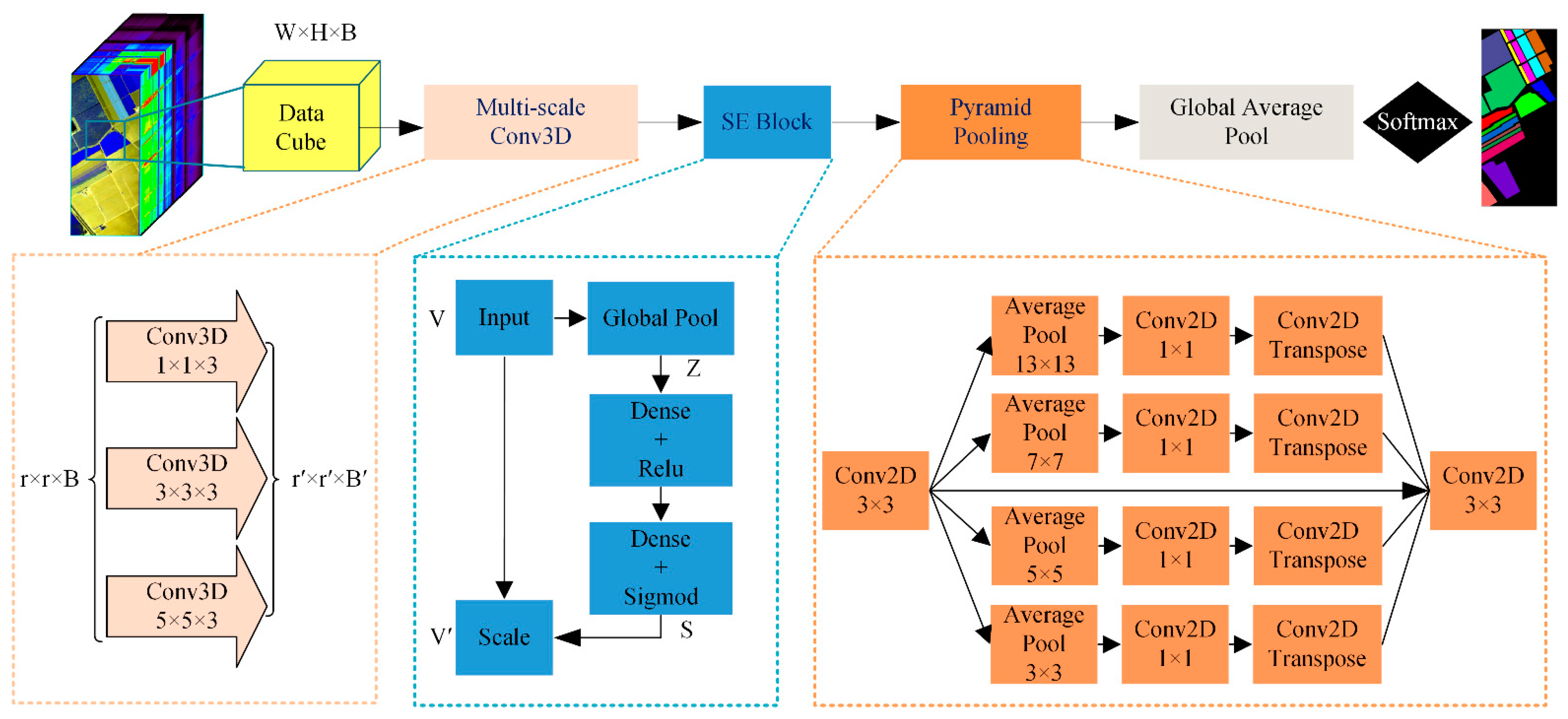
  • To overcome the “small sample problem” of hyperspectral pixel-level classification, we designed a multiscale information fusion hybrid 2D-3D CNN named the multiscale squeeze-and-excitation pyramid pooling network (MSPN) model to improve the classification performance. The model can not only deepen the network vertically, but can also expand the multiscale spectral–spatial information horizontally. In terms of being lightweight, the frequently used fully connected layer at the tail is replaced for the first time by a global average pooling layer to reduce model parameters.
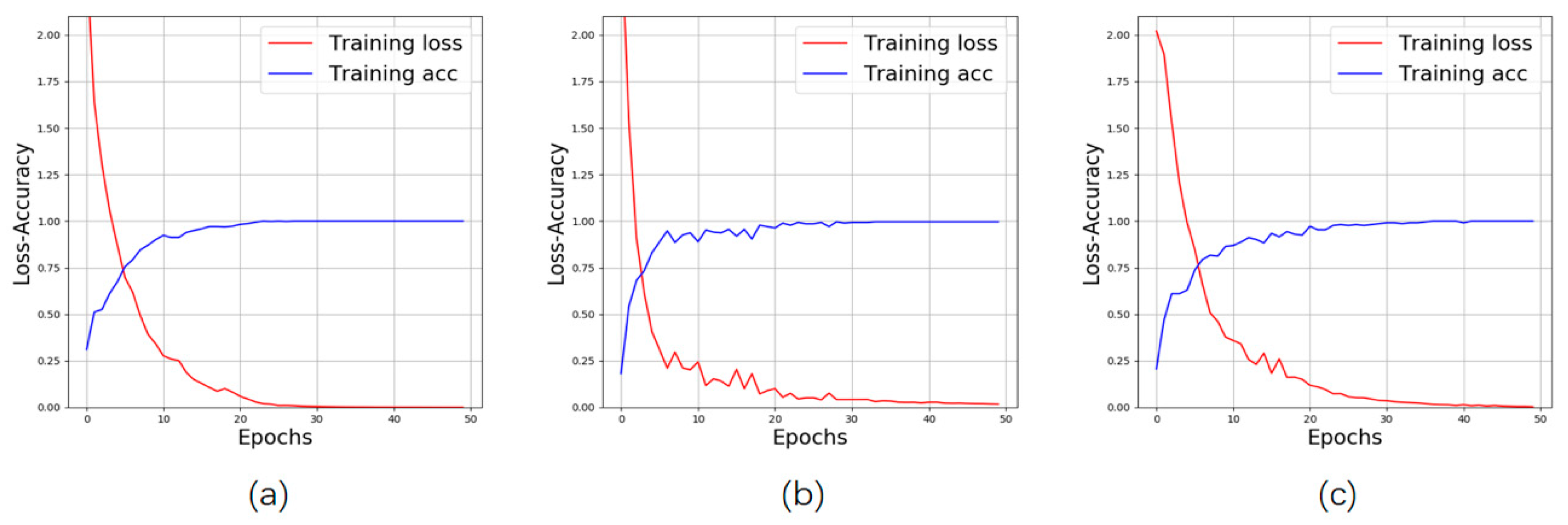
  • The proposed MSPN was trained on a small sample with 5%, 0.5%, and 0.5% of the labeled data from the three public datasets of Indian Pine, Salinas, and Pavia University, respectively. The prediction accuracies reached up to 96.09%, 97%, and 96.56%, respectively. The MSPN achieved high classification performance on the small sample.
This paper is organized as follows: Section 2 describes the proposed framework of the MSPN. Section 3 introduces the datasets used in the experiment. Section 4 describes the comparison experiments with existing methods and analyzes and discusses the results. Section 5 concludes the paper and looks at future research directions.

2. Methodology

Figure 1 shows the whole framework of the hyperspectral image classification based on the MSPN. First, dimension reduction is conducted on raw hyperspectral data using PCA and a relatively small number of principal components are kept. The number of retained principal components should have an error of no more than 0.01 in projecting the data from higher to lower dimensions, which means that 99% of the information is retained in the reduced dimensional data. Hyperspectral data can be regarded as a 3D cube with input space X N W × H × K , where W, H, and K are the width, height, and band, respectively. After selecting the first B principal components, the hyperspectral data can be denoted as N W × H × B . Next, the hyperspectral image cube is cut into small nearest-neighbor patches P i , j N r × r × B , where Pi, j represents the central pixel position at ( i , j ) with a window size of r × r covering all spectral dimensions B, composed of pixels from ( i ( r / 2 ) , j ( r / 2 ) ) to ( i + ( r / 2 ) , j ( r / 2 ) ) and from ( i ( r / 2 ) , j + ( r / 2 ) ) to ( i + ( r / 2 ) , j + ( r / 2 ) ) . The head of the MSPN is a multiscale 3D-CNN and accepts the 3D hyperspectral image patch as input. The output space for pixel-level classification is represented as Y L W × H , where L = { y 0 , y 1 , y k } is a set of possible categories. In order to determine whether the model has converged in the training stage, the difference between the predicted class labels L ^ = { y ^ 0 , y ^ 1 , y ^ k } and the ground truth class labels L = { y 0 , y 1 , y k } is estimated using a cross-entropy loss function:
C ( L ^ , L ) = i = 0 k y i ( log j = 0 k e y ^ j y ^ j )
The model would be optimized by iteratively updating the parameters through a backpropagation algorithm. The MSPN mainly includes three modules: a multiscale 3D-CNN module, an SE block, and a pyramid pooling module. The multiscale 3D-CNN, consisting of three parallel 3D convolution kernels, is used to extract preliminary spatial–spectral features. The data dimension from the 3D-CNN should be reshaped in order to input into the SE block, which focuses on the attention redistribution of spatial–spectral channel information. The pyramid pooling module further integrates spatial context information. Finally, the global pooling layer is used to replace the full connectivity layer and then reduce trainable parameters for avoiding overfitting. Each module is described in detail as follows.

2.1. Multiscale 3D-CNN

Multiscale convolution means that convolution kernels of different sizes are used simultaneously to learn multiscale information [42]. Multiscale information has been applied to the classification due to its rich context information in multiscale structures [43]. The multiscale convolution block can construct a more powerful network model for hyperspectral detection and classification [44]. Our proposed multiscale 3D-CNN consists of n = 3 parallel convolution kernels with different sizes k × k × d , and would extract three feature cubes with the size of r × r × B , such as 13 × 13 × 16, in our experiment. Simultaneously, the position ( x , y , z ) of each feature cube V is calculated as follows:
V i j x y z = μ ( m = 0 M i 1 b = 0 B i 1 h = 0 H i 1 w = 0 W i 1 K i j m h w b V ( i - 1 ) m ( x + h ) ( y + w ) ( z + b ) + R i j )
where K and R are the parameters of the convolution kernel and the bias term, respectively; i, j, and m are the indexes of input layer, output layer, and feature map, respectively; and μ is the activation function, such as the widely used rectified linear unit (ReLU). The input of the 3D-CNN is the small nearest-neighbor patches with the size of r × r × B , the subsampling steps of the 3D-CNN is ( s 1 , s 1 , s 2 ) . Then, the output spatial width is r = [ 1 + ( r k + 1 ) / s 1 ] , and the spectral depth is B = [ 1 + ( B d + 1 ) / s 2 ] . Let s 1 = s 2 = 1 and add the same padding operation to ensure that the output size is equal to the input size. Then, we concatenate the outputs of the three multiscale 3D-CNNs on the channel dimension and feed them into the SE block.

2.2. SE Block

The original generation of the SE block is used to improve network performance by explicitly simulating interdependencies between channels and adaptively recalibrating the characteristic response in terms of channels [45]. Due to the lightweight advantage of the SE block, it also can reduce model parameters and increase detection speed. A learning framework with an SE block can well characterize channel-wise spectral–spatial features [46]. Usually, an SE block includes two steps of squeeze and excitation. The squeeze operation firstly compresses the features along the spatial dimension. It turns each 2D feature channel into a real number, which has a global receptive field to some extent. The statistic Z of channel dimensions is generated by reducing the spatial dimension H × W of the reshaped feature cube V using global average pooling. The element of Z is calculated as follows:
Z = f s q ( V ) = 1 H × W α = 1 H β = 1 W V ( α , β )
Once the global spatial information is embedded into the feature vector Z N 1 × 1 × B , the excitation operation is used to convert the feature vector Z to another feature vector S as follows:
S = f e x ( Z , ω ) = σ ( μ ( Z , ω ) ) = σ ( ω 2 μ ( ω 1 Z ) )
where μ and σ are the ReLU activation function and sigmoid activation function, respectively; ω1 and ω2 represent the weights of two consecutive fully connected layers. The weights are automatically generated by learning the correlation between feature channels explicitly. The output feature channels of S match the input feature channels of Z. The above two operations can let the output vector S obtain the global information distribution. They can select the feature channels with more information by turning weights. Finally, the original feature cube V is recalibrated on the channel dimension by weighting the feature vector S via multiplication as follows:
V = f s c a l e ( V , S ) = S V
Accordingly, the SE block can extract the important information of feature channels automatically and then enhance the selected features and suppress the unusable features.

2.3. Pyramid Pooling Module

The pyramid pooling module can further integrate spatial information. It is usually used for scene parsing on image semantic segmentation [47] or pattern recognition [48], since it can aggregate multiple receptive fields in different scales. Furthermore, different scales of receptive field can gather richer spatial context information. In terms of this point, it is reasonable for us to employ it to address the limitations of single-size receptive fields in “small sample problems” of the hyperspectral image classification task and to improve classification accuracy. In this paper, the framework and parameters of the pyramid pooling module are specified as follows. A 2D convolutional layer with a kernel size of 3 × 3 and 128 channels is used to extract a feature map before pyramid pooling layers. Then, four pool layers with different receptive fields are used to downsample the feature map to different scales. The sizes of the four pooling layers are 13 × 13, 7 × 7, 5 × 5, and 3 × 3. Subsequently, the 1 × 1 convolution layer is used to change the number of channels. Then, the four downsampled feature maps are restored to the original size by the deconvolution layer. The original feature map and the restored four feature maps are concatenated in the channel dimension. The last 2D convolution layer with a kernel size of 3 × 3 and 256 channels is used to extract the final features, which provide rich global context information for pixel-level classification, even if there is the “small sample problem”.

3. Datasets and Details

To verify the proposed model, we used four publicly available hyperspectral datasets, namely the Indian Pine, Salinas, Pavia University, and WHU-Hi-LongKou datasets [49]. Some open codes were used for comparative experiments on the same training and test data. We adjusted the hyperparameters of the MSPN model using only the three classic datasets and then used the optimal model to challenge the latest high-resolution WHU-Hi-LongKou dataset. The open codes are available online at https://github.com/gokriznastic/HybridSN (accessed on 4 March 2021) and https://github.com/eecn/Hyperspectral-Classification (accessed on 4 March 2021). The WHU-Hi-LongKou dataset is available online at http://rsidea.whu.edu.cn/resource_WHUHi_sharing.htm (accessed on 25 May 2021). The classes and the number of samples for the four datasets are listed in Table 1.
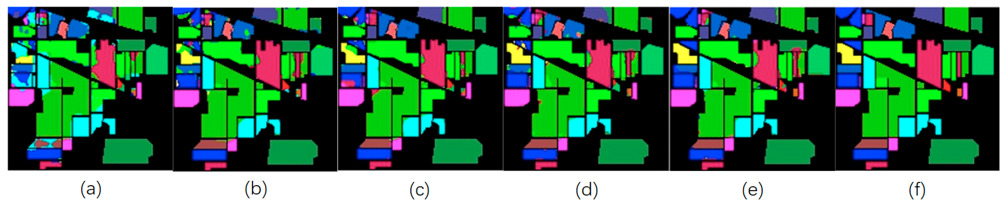
  • Each Indian Pine hyperspectral image is composed of 145 × 145 pixels with a spatial resolution of 20 m. The bands covering the water-absorbing area are removed, and the remaining 200 bands are used for classification. Indian Pine landscape mainly includes different types of crops, forests, and other perennial plants. The ground truth values are specified into 16 classes. The number of available sample points for all classes is 10,249. Each class includes a minimum of 20 and a maximum of 2455 sample points. As such, the distribution of sample points is very uneven. In addition, the crops are divided into two classes due to the different levels of tillage. For example, the first class is no-till corn and the second class is low-till corn. Both of them are cornfields.
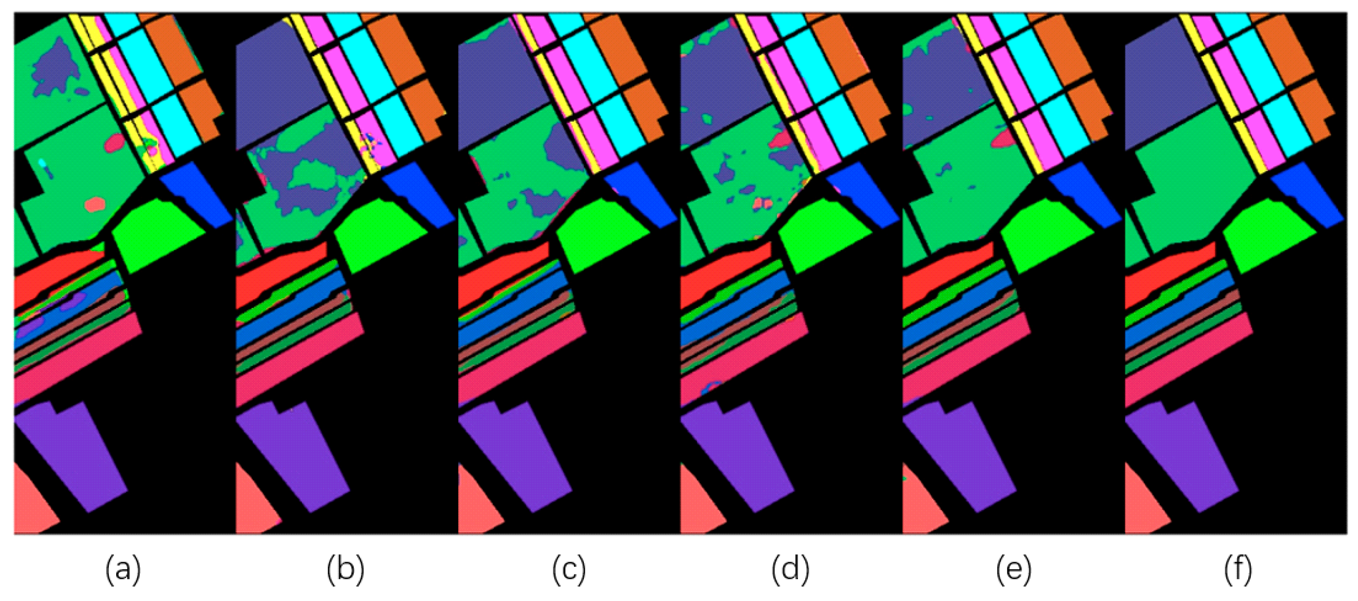
  • Each Salinas hyperspectral image consists of 512 × 217 pixels with a spatial resolution of 3.7 m. Similar to the Indian Pine images, the water absorption band is discarded and 204 bands remain. The Salinas scenes mainly include vegetation, bare soil, and vineyards. A total of 54,129 sample points are divided into 16 groups. Per class, the minimum number of sample points is 916 and the maximum number is 11,271, which is rather uneven. The Salinas dataset differs from the Indian Pine dataset in that there are more available labeled sample points and the spatial resolution is higher. There is also a similarity between several classes, e.g., classes 11, 12, 13, and 14 are longleaf lettuces, but they are divided into four classes depending on growth time. The advantage of this dataset is the high spatial resolution, which can help to improve the classification effect.
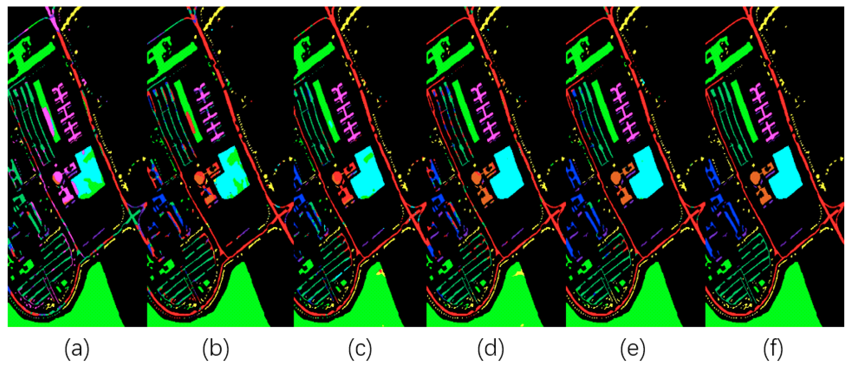
  • Each Pavia University hyperspectral image consists of 610 × 340 pixels with a spatial resolution of 1.3 m. The dataset includes 103 spectral bands. The labeled samples are divided into nine classes. The scenes mainly include urban features, such as metal sheets, roofs, asphalt pavements, etc. Per class, the minimum number of sample points is 947 and the maximum number is 18,649. The total number of labeled sample points is 42,776.
  • The WHU-Hi-LongKou dataset was acquired in 2018 in Longkou Town, China. Each hyperspectral image consists of 550 × 400 pixels with 270 bands from 400 to 1000 nm, and the spatial resolution of the hyperspectral imagery is about 0.463 m. It contains nine classes, namely Corn, Cotton, Sesame, Broad-leaf soybean, Narrow-leaf soybean, Rice, Water, Roads and houses, and Mixed weed. The minimum number of sample points is 3031 and the maximum number is 67,056. The total number of labeled sample points is 204,542.
For the supervised hyperspectral image classification, to our knowledge, the number of training sample points has a significant influence on the classification accuracy. To verify the effectiveness of the MSPN model with the “small sample problem”, we randomly selected 5% of sample points from the Indian Pine dataset, 0.5% of sample points from the Salinas dataset, and 0.5% of sample points from the Pavia University dataset as training samples and ensures that all classes were included. Since the Indian Pine dataset has an extremely uneven distribution of sample points, more training sample points (i.e., 5%) should be used to ensure that all classes are considered. For the other two datasets, since the sample points are rich and relatively uniform, use of fewer training sample points (i.e., 0.5%) is acceptable. For example, both the HybridSN [36] and R-HybridSN [37] models used 1% of sample points from these two datasets to train the networks and achieve a better classification accuracy. However, for the high-resolution WHU-Hi-LongKou dataset, since it has more training sample points, we took only 0.1% of them as training samples to highlight the performance of our model in regard to the “small sample problem”.

4. Results of Experiment

In order to evaluate the performance of the proposed MSPN model and compare it with other supervised deep learning methods, the following five experiments were implemented.
  • The first experiment evaluated the classification performances of the proposed MSPN and other models in terms of overall accuracy (OA), average accuracy (AA), and kappa coefficient, using a different number of training samples of the three classic datasets.
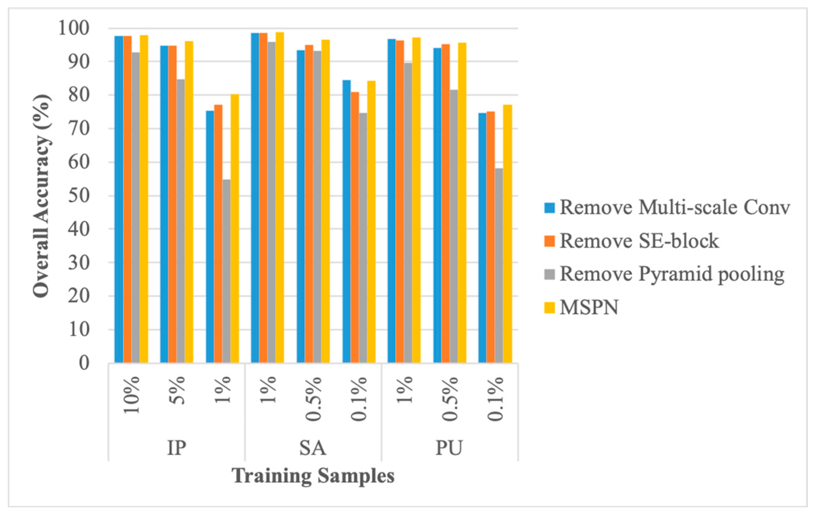
  • The second experiment compared the classification performances of the original MSPN model and its variants, such as by removing the multiscale 3D-CNN, SE block, or pyramid pooling module.
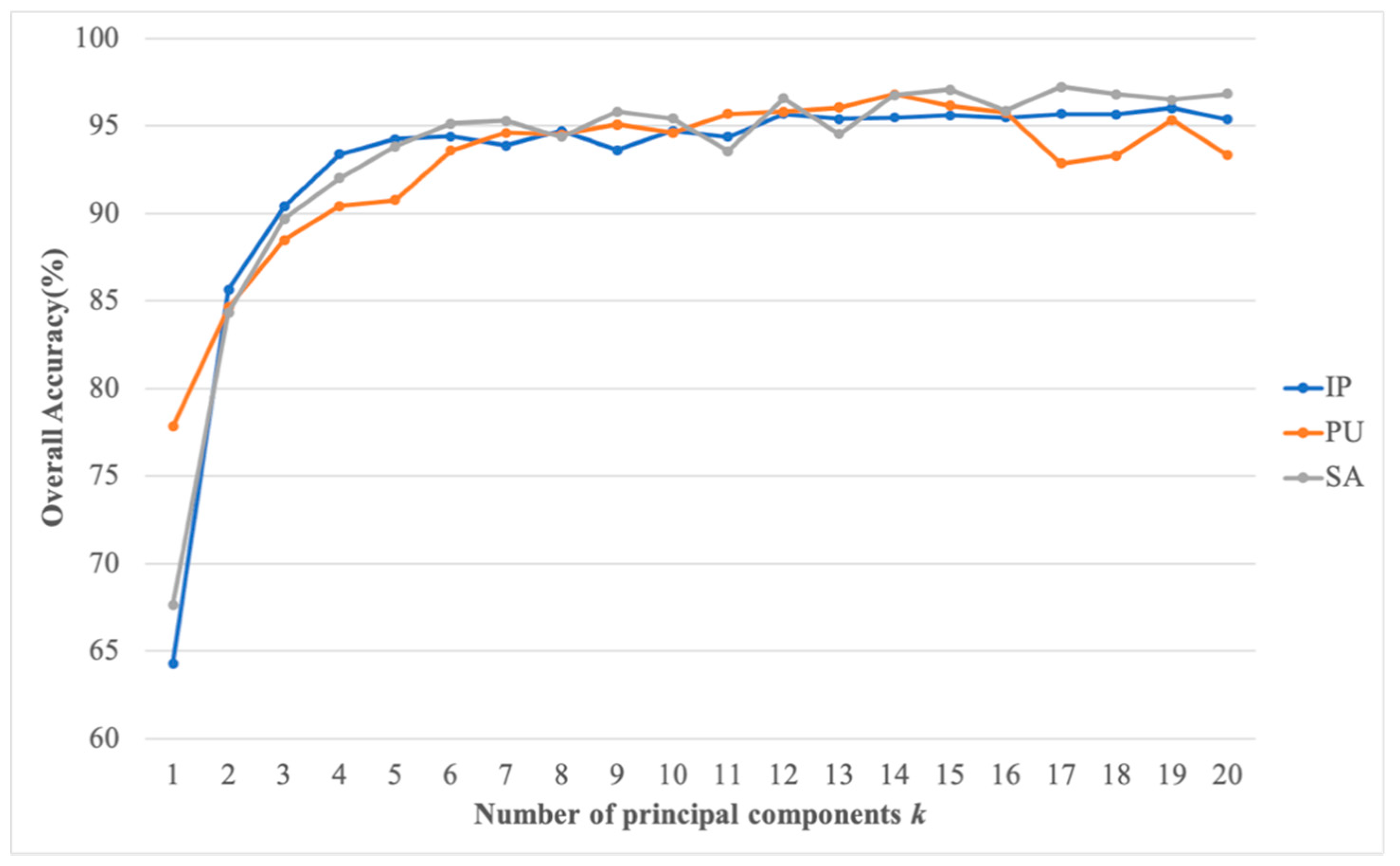
  • The third experiment verified the influence of the selection of principal components on the model performance.
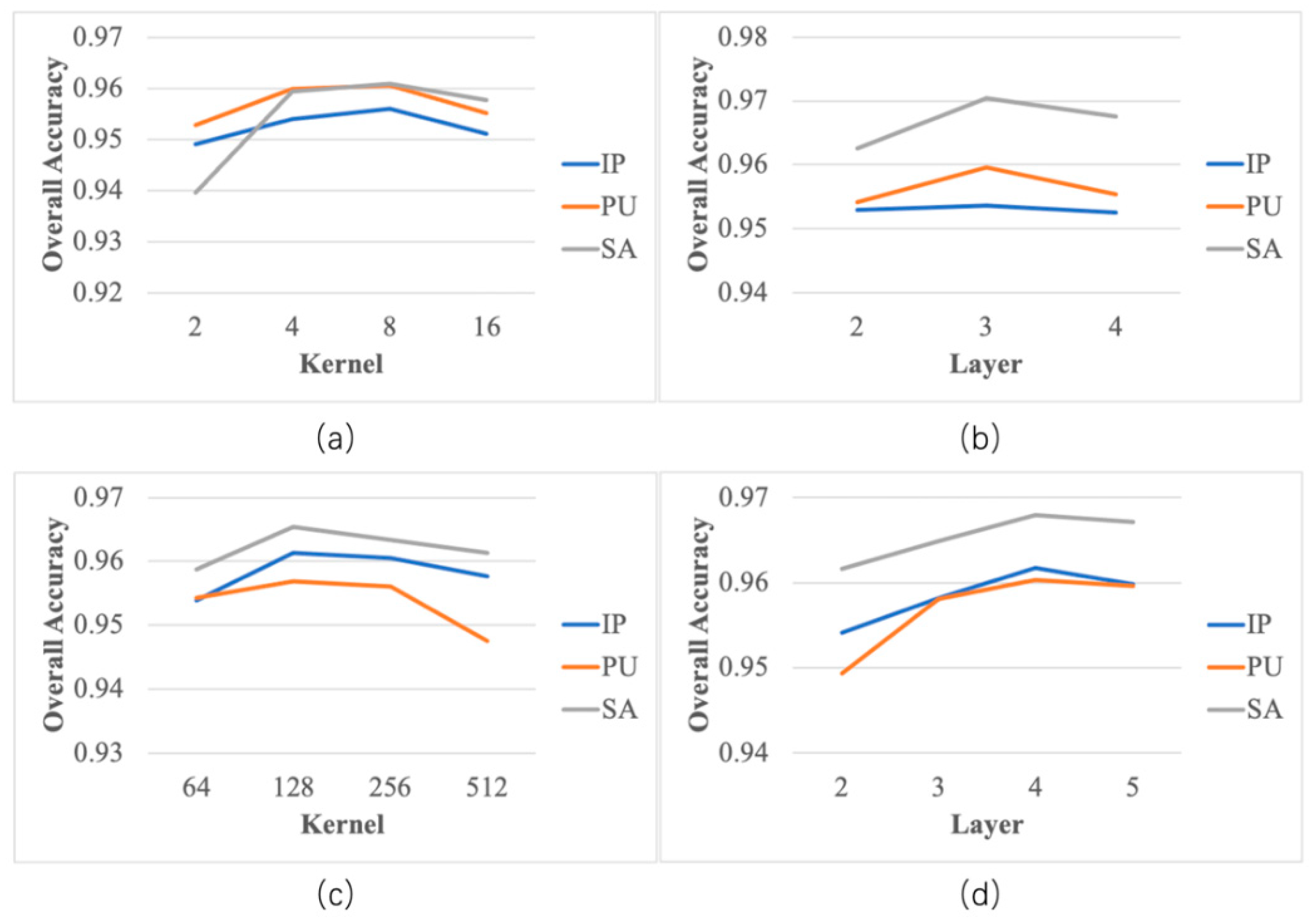
  • The fourth experiment determined the proper number of convolutional kernels and the number of parallel convolutional layers.
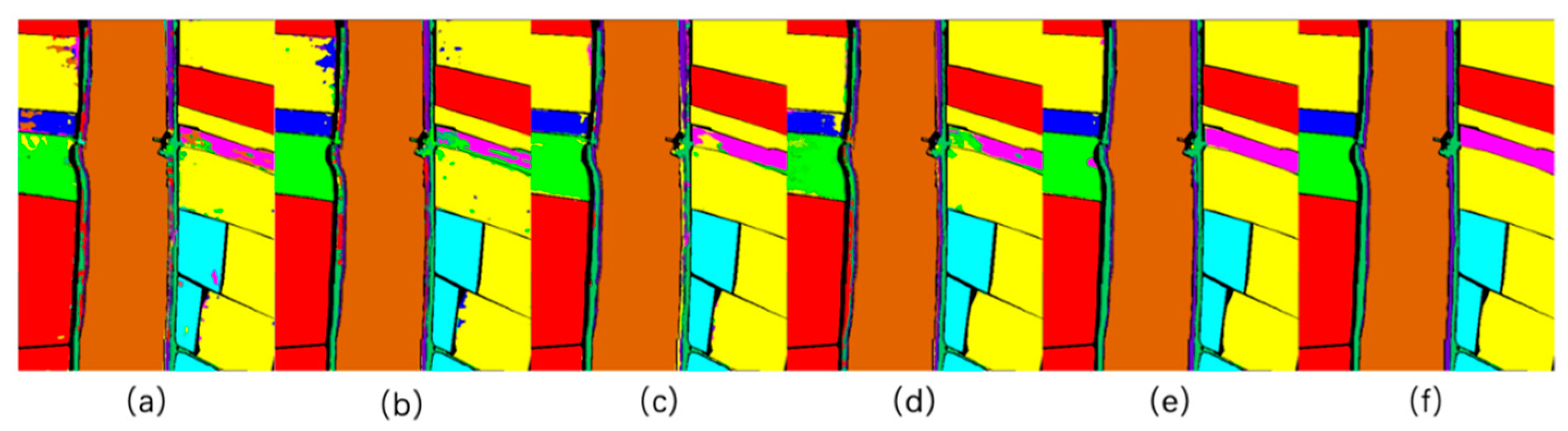
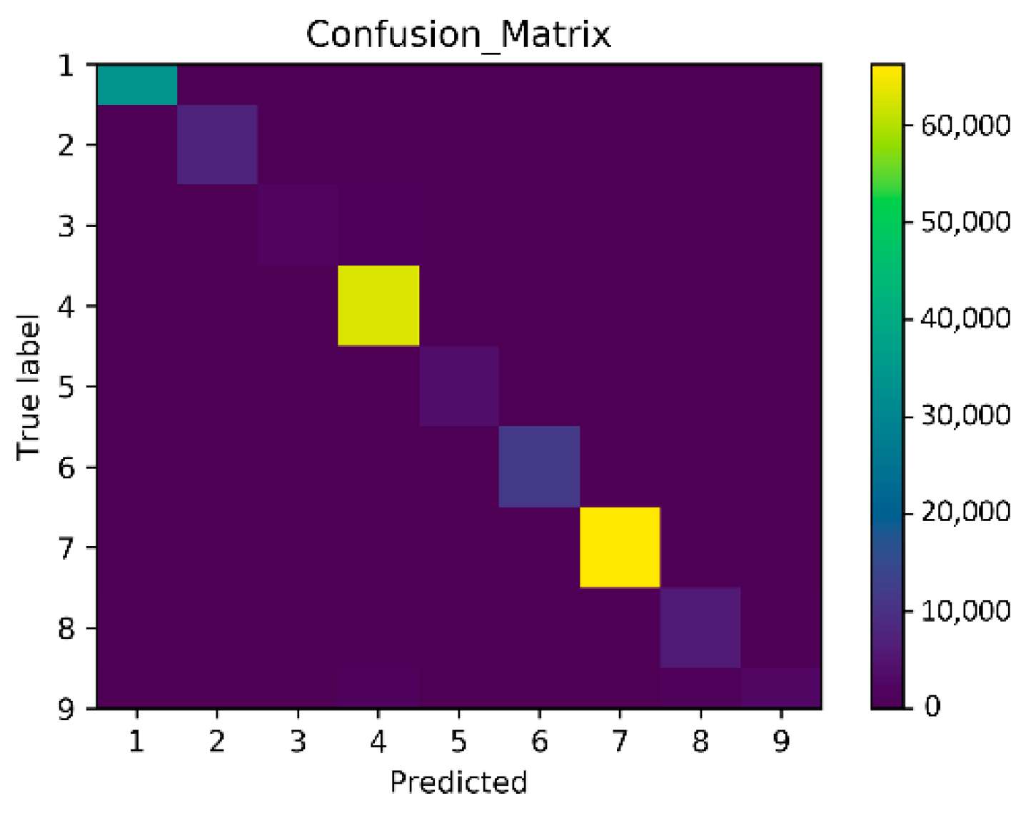
  • The fifth experiment aimed to challenge the latest high-resolution remote sensing images in the WHU-Hi-LongKou dataset. We compared our proposed MSPN model with other methods by taking 0.1% of the sample points as a training sample. At the same time, a confusion matrix was used to visualize the classification results of our proposed model.
The performance was evaluated by the indicators OA, AA, and kappa coefficient, where OA is the ratio of correctly classified pixels to total pixels, AA is the average value of classification accuracy, and the kappa coefficient is a metric of statistical measurement that can measure the consistency between a predicted map and the ground truth. The experiments were implemented with Tensorflow. We used mini-batches of size 128 for training the network. The optimizer was Adam, and the learning rate was set to 0.001. All experiments were repeated 10 times and the average value was taken as the final classification accuracy.
For the first experiment, Table 2, Table 3 and Table 4 list the classification performance of the different methods on all classes, and Figure 2, Figure 3 and Figure 4 show the ground truths and the predicted classification maps of the different models. Evidently, the classification maps and accuracy of the MSPN are better than those of the other models. It should be noted that the MSPN uses fixed hyperparameters for each dataset. That is, the MSPN has a good generalization ability for different hyperspectral images. The OA, AA, and kappa coefficient obtained by the MSPN were the highest relative to other models: the OA of the MSPN was 96.09% on the Indian Pine dataset, 97% on the Salinas dataset, and 96.56% on the Pavia University dataset. It is interesting to note that the hybrid 3D-CNN and 2D-CNN are superior to either the 2D-CNN or 3D-CNN alone. The addition of multiscale modules further improves the performance.
Figure 5 presents the convergence accuracy and loss on training phase over 50 epochs. Table 5 presents the computational efficiency of the MSPN in terms of training and testing time. As shown, the MSPN model is more efficient than the R-HybridSN model. Convergence was achieved after just 30 epochs, mainly because the full connection layer is replaced with the global pooling layer. In addition, relative to other models, the 3D-CNN layers are reduced, while the 2D-CNN layers are increased, and so the network becomes lightweight. There is no regularization strategy such as batch normalization and dropout.
In the second experiment, the contribution of each module was explored in detail. Removal of the multiscale module means letting the multiscale module become a single-scale one, and only the parameters of the middle 3D-CNN are copied. Removal of the SE block or pyramid pooling module means removing them from the network completely. Figure 6 shows the performance of the MSPN and its variants. The results show that the pyramid pooling module contributes the most to the model. When it is removed, the OA decreases the most, mainly because the module contains the most convolution layers and multiscale information. The SE block has the least impact because it only recalibrates the features from the spectral dimension to a certain extent. Compared with other modules, it only plays an auxiliary role in feature learning.
In the third experiment, the effect of the number of principal components on the classification performance was investigated. The fewer the principal components were, the fewer the spectral features and the shorter the computation time were, and vice versa. Figure 7 shows the classification OA as a function of the number of principal components. As expected, the OA increases with the number of principal components. However, the optimal principal components are different for different datasets. Considering generalization and stability, k = 16 is recommended. It should be note that PCA in preprocessing may lose part of the original hyperspectral data cube information. Therefore, it is necessary to explore new dimensionality reduction methods to reduce the parameters and retain the original information as much as possible in the future.
For the fourth experiment, Figure 8 shows the performance of different convolution kernels and parallel layers used in the MSPN. This experiment did not consider the SE block because it does not contain convolution layers. Based on the single variable principle, we used OA as the evaluation criterion. For the multiscale 3D-CNN, we changed the number of convolutional kernels per layer in the order of 2, 4, 8, and 16 in the case of determining three parallel convolutional layers. We changed the number of parallel convolution layers by copying or removing the middle branching layer in the case of determining eight kernels per layer. For the pyramid pooling module, the setting of variables was similar. The best parameters were determined in the multiscale 3D-CNN having three parallel layers with eight kernels per layer, and the pyramid pooling module having four parallel layers with 128 convolution kernels per layer. It should be noted that all the above determined optimal parameters were employed in the first experiment for comparison, and thus, the best classification performance was achieved.
For the fifth experiment, Table 6 lists the classification performance of different methods on all classes, and Figure 9 shows the ground truths and the predicted classification maps of the different models. Figure 10 shows the visualization of the confusion matrix. From these charts, we can see that our proposed model still performs better on the latest high-resolution WHU-Hi-LongKou dataset.

5. Conclusions

In this paper, to overcome the “small sample problem”, we proposed a multiscale squeeze-and-excitation pyramid pooling network (MSPN) model for hyperspectral image classification. The model includes a multiscale 3D-CNN module, an SE block, and a pyramid pooling module. The multiscale 3D-CNN can better integrate spatial–spectral information, and the SE block automatically relearns the information of the channel. The pyramid pooling module uses four pooling layers of different sizes and the corresponding convolution and deconvolution layers to extract spatial feature information, which can improve the robustness of the model to spatial layout and object variability. We implemented experiments on three public datasets, whereby it was proved that the combination of different multiscale modules can better learn spatial–spectral information in the case of small training samples. The contribution of each module to the model was defined. The pyramid pooling module contains the most convolution layers and multiscale information, therefore contributing the most, followed by the multiscale 3D-CNN. The SE block only plays an auxiliary role in the learning of features and contributes the least. The number of principal components, as well as the number of convolution layers and kernels on the test, was also determined. Overall, k = 16 principal components, a multiscale 3D-CNN module with three parallel layers and eight kernels per layer, and a pyramid pooling module with four parallel layers and 128 convolution kernels per layer are preferred. The proposed MSPN model shows competitive advantages in training and testing time and convergence speed and presents a superior performance on limited training samples compared with other similar methods. Compared with the existing methods, the purpose of our model is to utilize various effective modules to retrieve more information from limited training samples. In the future, transfer learning can be explored to improve the proposed model.

Author Contributions

Conceptualization, H.G. and T.M.; methodology, H.G. and Q.L.; software and experiments, H.G. and H.L.; validation, W.W., F.H., and A.T.; writing—original draft preparation, H.G.; writing—review and editing, T.M.; funding acquisition, T.M., C.L., H.D., and Z.H. All authors contributed to the results analysis and reviewed the manuscript. All authors have read and agreed to the published version of the manuscript.

Funding

This research was funded by the National Natural Science Foundation of China (NSFC) under Grant no. 61775176, in part by the National Major Special Projects of China under Grant GFZX04014308, in part by the Shaanxi Province Key Research and Development Program of China under Grants 2020GY-131 and 2021SF-135, in part by the Fundamental Research Funds for the Central Universities under Grant xjh012020021, and in part by the Natural Science Foundation of Shanghai under Grant 18ZR1437200.

Acknowledgments

The authors would like to thank M. Graña, MA. Veganzons, and B. Ayerdi for collecting the hyperspectral datasets and free downloads from http://www.ehu.eus/ccwintco/indexphp/Hyperspectral_Remote_Sensing_Scenes (accessed on 21 June 2019). The authors are grateful to the editor and reviewers for their constructive comments, which have significantly improved this work.

Conflicts of Interest

The authors declare no conflict of interest.

References

  1. Huang, R.; He, M. Band selection based on feature weighting for classification of hyperspectral data. IEEE Geosci. Remote Sens. Lett. 2005, 2, 156–159. [Google Scholar] [CrossRef]
  2. Hang, L.; Zhang, L.; Tao, D.; Huang, X.; Du, B. Hyperspectral Remote Sensing Image Subpixel Target Detection Based on Supervised Metric Learning. IEEE Trans. Geosci. Remote Sens. 2013, 52, 4955–4965. [Google Scholar] [CrossRef]
  3. Luo, B.; Yang, C.; Chanussot, J.; Zhang, L. Crop yield estimation based on unsupervised linear unmixing of multidate hyperspectral imagery. IEEE Trans. Geosci. Remote Sens. 2013, 51, 162–173. [Google Scholar] [CrossRef]
  4. He, L.; Li, J.; Plaza, A.; Li, Y. Discriminative Low-Rank Gabor Filtering for Spectral-Spatial Hyperspectral Image Classification. IEEE Trans. Geosci. Remote Sens. 2017, 55, 1381–1395. [Google Scholar] [CrossRef]
  5. Lowe, D.G. Distinctive Image Features from Scale-Invariant Keypoints. Int. J. Comput. Vis. 2004, 60, 91–110. [Google Scholar] [CrossRef]
  6. Dalal, N.; Triggs, B. Histograms of oriented gradients for human detection. In Proceedings of the IEEE Conference on Computer Vision and Pattern Recognition, San Diego, CA, USA, 20–25 June 2005; pp. 886–893. [Google Scholar]
  7. Pietikäinen, M. Local Binary Patterns. Scholarpedia 2010, 5, 9775. [Google Scholar] [CrossRef]
  8. Li, J.; Bioucas-Dias, J.M.; Plaza, A. Semisupervised hyperspec- tral image segmentation using multinomial logistic regression with active learning. IEEE Trans. Geosci. Remote Sens. 2010, 48, 4085–4098. [Google Scholar]
  9. Li, J.; Bioucas-Dias, J.M.; Plaza, A. Hyperspectral image segmen- tation using a new Bayesian approach with active learning. IEEE Trans. Geosci. Remote Sens. 2011, 49, 3947–3960. [Google Scholar] [CrossRef] [Green Version]
  10. Huang, K.; Li, S.; Kang, X.; Fang, L. Spectral–Spatial Hyperspectral Image Classification Based on KNN. Sens. Imaging Int. J. 2016, 17, 1–13. [Google Scholar] [CrossRef]
  11. Melgani, F.; Bruzzone, L. Classification of hyperspectral remote sensing images with support vector machines. IEEE Trans. Geosci. Remote Sens. 2004, 42, 1778–1790. [Google Scholar] [CrossRef] [Green Version]
  12. Arvelyna, Y.; Shuichi, M.; Atsushi, M.; Nguno, A.; Mhopjeni, K.; Muyongo, A.; Sibeso, M.; Muvangua, E. Hyperspectral mapping for rock and alteration mineral with Spectral Angle Mapping and Neural Network classification method: Study case in Warmbad district, south of Namibia. In Proceedings of the 2011 IEEE International Geoscience and Remote Sensing Symposium, Vancouver, BC, Canada, 24–29 July 2011; pp. 1752–1754. [Google Scholar]
  13. Licciardi, G.; Marpu, P.R.; Chanussot, J.; Benediktsson, J.A. Linear versus nonlinear PCA for the classification of hyperspectral data based on the extended morphological profiles. IEEE Geosci. Remote Sens. Lett. 2012, 9, 447–451. [Google Scholar] [CrossRef] [Green Version]
  14. Villa, A.; Benediktsson, J.A.; Chanussot, J.; Jutten, C. Hyper- spectral image classification with independent component discrimi- nant analysis. IEEE Trans. Geosci. Remote Sens. 2011, 49, 4865–4876. [Google Scholar] [CrossRef] [Green Version]
  15. Bandos, T.V.; Bruzzone, L.; Camps-Valls, G. Classification of hyperspectral images with regularized linear discriminant analysis. IEEE Trans. Geosci. Remote Sens. 2009, 47, 862–873. [Google Scholar] [CrossRef]
  16. Fauvel, M.; Tarabalka, Y.; Benediktsson, J.A.; Chanussot, J.; Tilton, J.C. Advances in spectral-spatial classification of hyperspectral images. Proc. IEEE 2013, 101, 652–675. [Google Scholar] [CrossRef] [Green Version]
  17. Jia, S.; Shen, L.; Li, Q. Gabor feature-based collaborative repre- sentation for hyperspectral imagery classification. IEEE Trans. Geosci. Remote Sens. 2015, 53, 1118–1129. [Google Scholar]
  18. Li, J.; Du, Q.; Li, Y.; Li, W. Hyperspectral image classification with imbalanced data based on orthogonal complement subspace projection. IEEE Trans. Geosci. Remote Sens. 2018, 56, 3838–3851. [Google Scholar] [CrossRef]
  19. Szegedy, C.; Liu, W.; Jia, Y.; Sermanet, P.; Reed, S.; Anguelov, D.; Erhan, D.; Vanhoucke, V.; Rabinovich, A. Going Deeper with Convolutions. In Proceedings of the 2015 IEEE Conference on Computer Vision and Pattern Recognition (CVPR), Boston, MA, USA, 7–12 June 2015; pp. 1–9. [Google Scholar]
  20. Redmon, J.; Divvala, S.; Girshick, R.; Farhadi, A. You only look once: Unified, real-time object detection. In Proceedings of the IEEE Conference on Computer Vision and Pattern Recognition, Las Vegas, NV, USA, 27–30 June 2016; pp. 779–788. [Google Scholar]
  21. Bordes, A.; Glorot, X.; Weston, J.; Bengio, Y. Joint learning of words and meaning representations for open-text semantic parsing. In Proceedings of the Fifteenth International Conference on Artificial Intelligence and Statistics, La Palma, Canary Islands, 12–15 April 2012; pp. 127–135. [Google Scholar]
  22. Krizhevsky, A.; Sutskever, I.; Hinton, G.E. Imagenet classification with deep convolutional neural networks. Commun. ACM 2012, 60, 1097–1105. [Google Scholar] [CrossRef]
  23. Li, S.; Song, W.; Fang, L.; Chen, Y.; Ghamisi, P.; Benediktsson, J.A. Deep Learning for Hyperspectral Image Classification: An Overview. IEEE Trans. Geosci. Remote Sens. 2019, 57, 6690–6709. [Google Scholar] [CrossRef] [Green Version]
  24. Chen, Y.; Lin, Z.; Zhao, X.; Wang, G.; Gu, Y. Deep Learning-Based Classification of Hyperspectral Data. IEEE J. Sel. Top. Appl. Earth Obs. Remote Sens. 2014, 7, 2094–2107. [Google Scholar] [CrossRef]
  25. Chen, Y.; Zhao, X.; Jia, X. Spectral-spatial classification of hyper- spectral data based on deep belief network. IEEE J. Sel. Topics Appl. Earth Observ. Remote Sens. 2015, 8, 2381–2392. [Google Scholar] [CrossRef]
  26. Hu, W.; Huang, Y.; Wei, L.; Zhang, F.; Li, H.-C. Deep Convolutional Neural Networks for Hyperspectral Image Classification. J. Sensors 2015, 2015, 1–12. [Google Scholar] [CrossRef] [Green Version]
  27. Makantasis, K.; Karantzalos, K.; Doulamis, A.; Doulamis, N. Deep supervised learning for hyperspectral data classification through con volutional neural networks. In Proceedings of the 2015 IEEE International Geoscience and Remote Sensing Symposium, Milan, Italy, 26–31 July 2015; pp. 4959–4962. [Google Scholar]
  28. Zhu, J.; Fang, L.; Ghamisi, P. Deformable Convolutional Neural Networks for Hyperspectral Image Classification. IEEE Geosci. Remote Sens. Lett. 2018, 15, 1254–1258. [Google Scholar] [CrossRef]
  29. Pan, B.; Xu, X.; Shi, Z.; Zhang, N.; Luo, H.; Lan, X. DSSNet: A Simple Dilated Semantic Segmentation Network for Hyperspectral Imagery Classification. IEEE Geosci. Remote Sens. Lett. 2020, 17, 1968–1972. [Google Scholar] [CrossRef]
  30. Li, X.; Ding, M.; Pižurica, A. Deep Feature Fusion via Two-Stream Convolutional Neural Network for Hyperspectral Image Classification. IEEE Trans. Geosci. Remote Sens. 2020, 58, 2615–2629. [Google Scholar] [CrossRef] [Green Version]
  31. Song, W.; Li, S.; Fang, L.; Lu, T. Hyperspectral Image Classification with Deep Feature Fusion Network. IEEE Trans. Geosci. Remote Sens. 2018, 56, 3173–3184. [Google Scholar] [CrossRef]
  32. Chen, Y.; Jiang, H.; Li, C.; Jia, X.; Ghamisi, P. Deep Feature Extraction and Classification of Hyperspectral Images Based on Convolutional Neural Networks. IEEE Trans. Geosci. Remote Sens. 2016, 54, 6232–6251. [Google Scholar] [CrossRef] [Green Version]
  33. Zhong, Z.; Li, J.; Luo, Z.; Chapman, M. Spectral–Spatial Residual Network for Hyperspectral Image Classification: A 3-D Deep Learning Framework. IEEE Trans. Geosci. Remote Sens. 2017, 56, 847–858. [Google Scholar] [CrossRef]
  34. He, M.; Li, B.; Chen, H. Multi-scale 3D deep convolutional neural network for hyperspectral image classification. In Proceedings of the 2017 IEEE International Conference on Image Processing (ICIP), Beijing, China, 17–20 September 2017; pp. 3904–3908. [Google Scholar]
  35. Sellami, A.; Ben Abbes, A.; Barra, V.; Farah, I.R. Fused 3-D spectral-spatial deep neural networks and spectral clustering for hyperspectral image classification. Pattern Recognit. Lett. 2020, 138, 594–600. [Google Scholar] [CrossRef]
  36. Paoletti, M.E.; Haut, J.M.; Fernandez-Beltran, R.; Plaza, J.; Plaza, A.J.; Pla, F. Deep Pyramidal Residual Networks for Spectral-Spatial Hyperspectral Image Classification. IEEE Trans. Geosci. Remote Sens. 2019, 57, 740–754. [Google Scholar] [CrossRef]
  37. Swalpa, K.R.; Gopal, K.; Shiv, R.D.; Bidyut, B.C. HybridSN: Exploring 3-D-2-D CNN Feature Hierarchy for Hyperspectral Image Classification. IEEE Geosci. Remote Sens. Lett. 2019, 17, 277–281. [Google Scholar]
  38. Feng, F.; Wang, S.; Wang, C.; Zhang, J. Learning Deep Hierarchical Spatial–Spectral Features for Hyperspectral Image Classification Based on Residual 3D-2D CNN. Sensors 2019, 19, 5276. [Google Scholar] [CrossRef] [Green Version]
  39. Ge, Z.; Cao, G.; Li, X.; Fu, P. Hyperspectral Image Classification Method Based on 2D–3D CNN and Multibranch Feature Fusion. IEEE J. Sel. Top. Appl. Earth Obs. Remote Sens. 2020, 13, 5776–5788. [Google Scholar] [CrossRef]
  40. Hu, J.; Shen, L.; Albanie, S.; Sun, G.; Wu, E. Squeeze-and-Excitation Networks. IEEE Trans. Pattern Anal. Mach. Intell. 2020, 42, 2011–2023. [Google Scholar] [CrossRef] [PubMed] [Green Version]
  41. Zhao, H.; Shi, J.; Qi, X.; Wang, X.; Jia, J. Pyramid Scene Parsing Network. In Proceedings of the 2017 IEEE Conference on Computer Vision and Pattern Recognition (CVPR), Honolulu, HI, USA, 21–26 July 2017; pp. 1063–6919. [Google Scholar]
  42. Liang, M.; Jiao, L.; Yang, S.; Liu, F.; Hou, B.; Chen, H. Deep multiscale spectral-spatial feature fusion for hyperspectral images classification. IEEE J. Sel. Topics Appl. Earth Observ. Remote Sens. 2018, 11, 2911–2924. [Google Scholar] [CrossRef]
  43. He, N.; Paoletti, M.E.; Haut, J.N.M.; Fang, L.; Li, S.; Plaza, A.; Plaza, J. Feature Extraction with Multiscale Covariance Maps for Hyperspectral Image Classification. IEEE Trans. Geosci. Remote Sens. 2019, 57, 755–769. [Google Scholar] [CrossRef]
  44. Gong, Z.; Zhong, P.; Yu, Y.; Hu, W.; Li, S. A CNN with Multiscale Convolution and Diversified Metric for Hyperspectral Image Classification. IEEE Trans. Geosci. Remote Sens. 2019, 57, 3599–3618. [Google Scholar] [CrossRef]
  45. Lin, Z.; Ji, K.; Leng, X.; Kuang, G. Squeeze and Excitation Rank Faster R-CNN for Ship Detection in SAR Images. IEEE Geosci. Remote Sens. Lett. 2019, 16, 751–755. [Google Scholar] [CrossRef]
  46. Roy, S.K.; Chatterjee, S.; Bhattacharyya, S.; Chaudhuri, B.B.; Platos, J. Lightweight Spectral–Spatial Squeeze-and- Excitation Residual Bag-of-Features Learning for Hyperspectral Classification. IEEE Trans. Geosci. Remote Sens. 2020, 58, 5277–5290. [Google Scholar] [CrossRef]
  47. Kim, J.H.; Lee, H.; Hong, S.J.; Kim, S.; Park, J.; Hwang, J.Y.; Choi, J.P. Objects Segmentation From High-Resolution Aerial Images Using U-Net With Pyramid Pooling Layers. IEEE Geosci. Remote Sens. Lett. 2018, 16, 115–119. [Google Scholar] [CrossRef]
  48. Gao, X.; Sun, X.; Zhang, Y.; Yan, M.; Xu, G.; Sun, H.; Jiao, J.; Fu, K. An End-to-End Neural Network for Road Extraction from Remote Sensing Imagery by Multiple Feature Pyramid Network. IEEE Access 2018, 6, 39401–39414. [Google Scholar] [CrossRef]
  49. Zhong, Y.; Hu, X.; Luo, C.; Wang, X.; Zhao, J.; Zhang, L. WHU-Hi: UAV-borne hyperspectral with high spatial resolution (H2) benchmark datasets and classifier for precise crop identification based on deep convolutional neural network with CRF. Remote Sens. Environ. 2020, 250, 112012. [Google Scholar] [CrossRef]
Figure 1. Illustration of the proposed model MSPN.
Remotesensing 13 02268 g001
Figure 2. The predicted classification maps for 5% samples from the Indian Pine dataset with the method of (a) 2D-CNN, (b) M3D-CNN, (c) HybridSN, (d) R-HybridSN, and (e) MSPN and (f) ground truth.
Remotesensing 13 02268 g002
Figure 3. The predicted classification map for 0.5% samples from the Salinas dataset with the method of (a) 2D-CNN, (b) M3D-CNN, (c) HybridSN, (d) R-HybridSN, and (e) MSPN and (f) ground truth.
Remotesensing 13 02268 g003
Figure 4. The predicted classification map for 0.5% samples from the Pavia University dataset with the method of (a) 2D-CNN, (b) M3D-CNN, (c) HybridSN, (d) R-HybridSN, and (e) MSPN and (f) ground truth.
Remotesensing 13 02268 g004
Figure 5. Training loss and accuracy convergence for (a) Indian Pine, (b) Salinas, and (c) Pavia University.
Remotesensing 13 02268 g005
Figure 6. OA of the MSPN while removing each module separately.
Remotesensing 13 02268 g006
Figure 7. OA of the MSPN using different numbers of principal components k.
Remotesensing 13 02268 g007
Figure 8. OA of the MSPN using different numbers of kernels and layers in each module. (a) The number of kernels in the multiscale 3D-CNN module. (b) The number of parallel layers in the multiscale 3D-CNN module. (c) The number of kernels in the pyramid pooling module. (d) The number of parallel layers in the pyramid pooling module.
Remotesensing 13 02268 g008
Figure 9. The predicted classification map for 0.1% samples from the WHU-Hi-LongKou dataset with the method of (a) 2D-CNN, (b) M3D-CNN, (c) HybridSN, (d) R-HybridSN, and (e) MSPN and (f) ground truth.
Remotesensing 13 02268 g009
Figure 10. The confusion matrix using the proposed method over 0.1% samples from the WHU-Hi-LongKou dataset.
Remotesensing 13 02268 g010
Table 1. Ground truth classes for all datasets and their respective sample numbers.
Indian PineSalinasPavia UniversityWHU-Hi-LongKou
OrderClassSamplesOrderClassSamplesOrderClassSamplesOrderClassSamples
1Alfalfa461Brocoli_green_weeds_120091Asphalt66311Corn34,511
2Corn-notill14282Brocoli_green_weeds_237262Meadows18,6492Cotton8374
3Corn-mintill8303Fallow19763Gravel20993Sesame3031
4Corn2374Fallow_rough_plow13944Trees30644Broad-leaf soybean63,212
5Grass-pasture4835Fallow_smooth26785Paintedmetalsheets13455Narrow-leaf soybean4151
6Grass-trees7306Stubble39596Bare Soil50296Rice11,854
7Grass-pasture-mowed287Celery35797Bitumen13307Water67,056
8Hay-windrowed4788Grapes_untrained11,2718Self-Blocking Bricks36828Roads and houses7124
9Oats209Soil_vinyard_develop62039Shadows9479Mixed weed5229
10Soybean-notill97210Corn_senesced_green_weeds3278
11Soybean-mintill245511Lettuce_romaine_4wk1068
12Soybean-clean59312Lettuce_romaine_5wk1927
13Wheat20513Lettuce_romaine_6wk916
14Woods126514Lettuce_romaine_7wk1070
15Buildings-Grass-Trees-Drives38615Vinyard_untrained7268
16Stone-Steel-Towers9316Vinyard_vertical_trellis1807
Table 2. Accuracy comparison of different methods for 5% samples of Indian Pine.
OrderClass2D-CNNM3D-CNNHybridSNR-HybridSNMSPN
1Alfalfa0.851.000.961.000.91
2Corn-notill0.850.900.920.900.95
3Corn-mintill0.910.940.970.980.95
4Corn0.920.870.980.921.00
5Grass-pasture0.910.990.940.980.97
6Grass-trees0.480.971.001.001.00
7Grass-pasture-mowed1.001.001.001.000.90
8Hay-windrowed0.901.000.950.911.00
9Oats0.000.930.751.000.93
10Soybean-notill0.980.920.880.870.90
11Soybean-mintill0.920.890.920.960.97
12Soybean-clean0.890.840.970.960.95
13Wheat0.981.001.000.950.99
14Woods1.000.970.990.930.98
15Buildings-Grass-Trees-Drives0.870.980.980.940.97
16Stone-Steel-Towers0.930.920.970.800.99
OA/% 85.5692.6594.1993.6696.09
Kappa/% 83.4991.5793.3492.7795.53
AA/% 71.4386.8386.7987.5791.53
Table 3. Accuracy comparison of different methods for 0.5% samples of Salinas.
OrderClass2D-CNNM3D-CNNHybridSNR-HybridSNMSPN
1Brocoli_green_weeds_10.941.000.981.001.00
2Brocoli_green_weeds_20.921.000.971.001.00
3Fallow1.000.951.001.001.00
4Fallow_rough_plow0.480.900.960.980.98
5Fallow_smooth1.000.981.000.910.97
6Stubble0.990.991.001.001.00
7Celery1.001.001.000.991.00
8Grapes_untrained0.640.920.990.950.94
9Soil_vinyard_develop0.910.990.951.000.99
10Corn_senesced_green_weeds0.881.001.000.900.90
11Lettuce_romaine_4wk1.000.991.000.961.00
12Lettuce_romaine_5wk0.990.911.000.861.00
13Lettuce_romaine_6wk0.910.890.740.760.91
14Lettuce_romaine_7wk1.000.910.870.830.90
15Vinyard_untrained0.940.600.840.850.98
16Vinyard_vertical_trellis0.871.001.000.861.00
OA/% 82.8889.6795.5293.5597.00
Kappa/% 80.7788.6095.0292.8396.66
AA/% 84.9195.3295.5793.2497.33
Table 4. Accuracy comparison of different methods for 0.5% samples of Pavia University.
OrderClass2D-CNNM3D-CNNHybridSNR-HybridSNMSPN
1Asphalt0.940.760.780.940.95
2Meadows0.900.850.940.990.98
3Gravel0.710.680.800.740.87
4Trees1.000.930.930.940.96
5Painted metal sheets0.261.000.930.991.00
6Bare Soil0.970.990.930.960.99
7Bitumen0.960.750.780.860.99
8Self-Blocking Bricks0.460.670.810.710.93
9Shadows0.350.540.970.840.95
OA/% 74.7781.9589.1092.5496.56
Kappa/% 66.5375.2185.3590.1295.42
AA/% 61.1068.2576.9289.5094.55
Table 5. Speed comparison of different methods in the Pavia University dataset with 0.5% training samples (processor: 1.8 GHz Intel Core i5, no GPU acceleration).
Train time/sTest time/s
2D-CNN418.41512.4
R-HybridSN332.31336.1
MSPN310.71035.5
Table 6. Accuracy comparison of different methods for 0.1% samples from the WHU-Hi-LongKou dataset.
OrderClass2D-CNNM3D-CNNHybridSNR-HybridSNMSPN
1Corn0.950.950.980.950.99
2Cotton0.910.830.930.750.94
3Sesame0.930.971.000.711.00
4Broad-leaf soybean0.970.970.950.990.96
5Narrow-leaf soybean0.760.960.810.960.84
6Rice0.970.990.960.991.00
7Water0.970.981.001.001.00
8Roads and houses0.840.850.840.830.91
9Mixed weed0.910.930.860.900.86
OA/% 95.4996.0496.3996.0397.31
Kappa/% 94.0594.7695.2494.7996.45
AA/% 84.3284.8786.6287.8189.82
Publisher’s Note: MDPI stays neutral with regard to jurisdictional claims in published maps and institutional affiliations.

