Abstract
An informative training set is necessary for ensuring the robust performance of the classification of very-high-resolution remote sensing (VHRRS) images, but labeling work is often difficult, expensive, and time-consuming. This makes active learning (AL) an important part of an image analysis framework. AL aims to efficiently build a representative and efficient library of training samples that are most informative for the underlying classification task, thereby minimizing the cost of obtaining labeled data. Based on ranked batch-mode active learning (RBMAL), this paper proposes a novel combined query strategy of spectral information divergence lowest confidence uncertainty sampling (SIDLC), called RBSIDLC. The base classifier of random forest (RF) is initialized by using a small initial training set, and each unlabeled sample is analyzed to obtain the classification uncertainty score. A spectral information divergence (SID) function is then used to calculate the similarity score, and according to the final score, the unlabeled samples are ranked in descending lists. The most “valuable” samples are selected according to ranked lists and then labeled by the analyst/expert (also called the oracle). Finally, these samples are added to the training set, and the RF is retrained for the next iteration. The whole procedure is iteratively implemented until a stopping criterion is met. The results indicate that RBSIDLC achieves high-precision extraction of urban land use information based on VHRRS; the accuracy of extraction for each land-use type is greater than 90%, and the overall accuracy (OA) is greater than 96%. After the SID replaces the Euclidean distance in the RBMAL algorithm, the RBSIDLC method greatly reduces the misclassification rate among different land types. Therefore, the similarity function based on SID performs better than that based on the Euclidean distance. In addition, the OA of RF classification is greater than 90%, suggesting that it is feasible to use RF to estimate the uncertainty score. Compared with the three single query strategies of other AL methods, sample labeling with the SIDLC combined query strategy yields a lower cost and higher quality, thus effectively reducing the misclassification rate of different land use types. For example, compared with the Batch_Based_Entropy (BBE) algorithm, RBSIDLC improves the precision of barren land extraction by 37% and that of vegetation by 14%. The 25 characteristics of different land use types screened by RF cross-validation (RFCV) combined with the permutation method exhibit an excellent separation degree, and the results provide the basis for VHRRS information extraction in urban land use settings based on RBSIDLC.
1. Introduction
Very-high-resolution remote sensing (VHRRS) images, which contain valuable features, particularly spatial information, have drawn much attention in urban land use monitoring in recent years [1,2,3,4,5,6]. Moreover, with the development of aerospace technology and sensor technology, VHRRS images are becoming increasingly easy and inexpensive to obtain, which raises the problem of enormous amounts of data being underutilized. Thus, unlabeled data are abundant, but labeling is time-consuming and expensive. Driven by the explosion of remotely sensed datasets, the establishment of accurate and effective methods for remotely sensed imagery information extraction is a prerequisite for applications and investigations of remote sensing technology.
The extraction methods of urban land use information mainly include support vector machines [7,8], decision trees [9], random forest (RF) models [10,11], and deep learning [12,13,14]. Most of these methods are based on supervised learning, which requires many labeled samples for model training [15]. Therefore, it is challenging to examine the training of classifiers with limited samples for the interpretation of remote sensing images [16]. Many scholars have explored methods to reduce the dependence of models on samples, such as transfer learning [17], few-shot learning [18], semi-supervised learning [19,20,21,22], unsupervised learning [23,24], and weakly supervised learning [25,26], and have achieved favorable results. However, the performance of these methods is not comparable to that of supervised learning methods.
Active learning (AL) finds the most “valuable” training samples through heuristic strategies and aims to achieve high accuracy using as few labeled samples as possible for the underlying classification task. It can achieve or even exceed the expected effect while minimizing the labeling cost [27,28,29,30]. This approach effectively solves the problem of classifier training with limited samples and has attracted attention from scholars worldwide [28,31,32]. To use AL on an unlabeled dataset, a very small sample of these data must first be labeled and a model must be trained. After the model is built, predictions should be made for all the unlabeled data. The labeling should be prioritized using a score. The selected sample should then be labeled and a model should be trained. The steps can be repeated iteratively to improve the model. AL includes two learning modes: stream-based selective sampling and pool-based sampling [33]. Stream-based selective sampling determines whether samples need to be labeled in sequence. The disadvantage is that it is impossible to obtain the structural distribution of samples. Pool-based sampling involves forming many unlabeled samples in the sample pool and then using a certain screening strategy to select the most “valuable” samples from the pool for priority labeling. However, there is a common problem between the two AL types; notably, only one sample can be selected for annotation in each iteration, resulting in exceedingly low efficiency. To improve the efficiency of AL sample labeling, researchers have proposed batch-mode active learning (BMAL) [34,35,36,37]. BMAL is a learning model based on a sample pool from which a batch of unlabeled samples is generated in each iteration. The samples are labeled through various methods, thus solving the problem of low sample labeling efficiency. However, BMAL only uses an active selection strategy based on a single uncertainty index or diversity index when screening samples, which leads to considerable information redundancy in the labeled samples and unnecessary labeling costs. Cardoso [38] proposed the ranked batch-mode active learning (RBMAL) framework, which overcomes the limitations of traditional BMAL methods and generates an optimized ranked list to determine the priority of samples being labeled. Therefore, the RBMAL method has higher flexibility than the classic methods.
The query strategy is a critical part of the AL method. The objective is to select valuable samples for model training, an approach which is directly related to reducing the cost of annotation. At present, the commonly used query strategies can be divided into uncertainty sampling methods and query-by-committee (QBC) methods. The uncertainty-based methods include least confidence [39], margin sampling [40], and entropy-based sampling [41], and the QBC methods include the vote entropy and Kullback–Leibler maximization methods. A single query strategy usually leads to sampling bias [42]; that is, the selected samples may not effectively reflect the distribution characteristics of the sample dataset. Therefore, combined query strategies have become popular [43,44].
In this study, we design a novel combined query strategy of spectral information divergence lowest confidence uncertainty sampling (SIDLC) based on RBMAL (RBSIDLC), to achieve high accuracy in extracting urban land use information from Worldview-3 VHRRS data by using as few labeled samples as possible. The combined query strategy, combining the RF as the base classifier for uncertainty estimation and a SID similarity measure function to form a novel query strategy, aimed to select the most informative and “valuable” samples for labeling. First, the RF is initialized with a few initial training sets, and the classification uncertainty score is obtained through the analyses of unlabeled samples. Then, the SID function is used to calculate the similarity score, and according to the final score, the unlabeled samples are ranked in a descending list. Third, the most uncertain samples are selected according to the ranked list and labeled by the oracle. Finally, after labeling, such samples are incorporated into the training set, which is used to retrain the RF in the next iteration until a satisfactory result is obtained. The research results would potentially introduce a new AL method and the AL-based VHRRS information extraction.
2. Materials and Methods
2.1. Study Area
The research area is the West Lake District of Hangzhou City, located in Zhejiang Province in Southeast China (Figure 1). The topography of the study area is plains, and rivers run vertically and horizontally, with a high degree of urbanization and highly complex ground features. There are mainly buildings with relatively regular shapes, grassland, barren land, large and regular street trees, regular roads, prominent small squares and playgrounds, etc. The main feature types basically cover the types of urban land. Although a standard Worldview-3 image has 8 MS bands with 1.24 m spatial resolution, and a panchromatic with 0.30 m spatial resolution [45], in this study, the collected Worldview-3 image over the study area was obtained on 28 October 2018, including four multispectral bands (R, G, B, and NIR) and one panchromatic band. The spatial resolution of the four multispectral bands is 2 m, and that of the panchromatic band is 0.5 m. ENVI 5.3 Gram–Schmidt pan sharpening [46] was used to fuse multispectral images with the panchromatic band to obtain a multispectral remote sensing image with a resolution of 0.5 m.
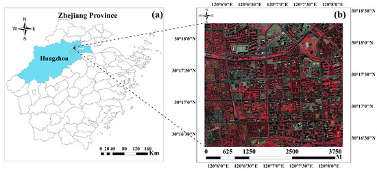
Figure 1.
Location of the study area: (a) Zhejiang Province. The blue polygon represents Hangzhou; (b) the subregion of the West Lake District of Hangzhou.
In this study, according to a field investigation, the USGS land cover classification system [47] and the FROM-GLC10 [48,49] classification system include five land cover types: barren land, built-up land, water, grassland, and forest. In addition, Figure 1b shows an image acquired on 28 October 2018. The solar elevation angle was approximately 46°, and consequently, the effects of shadowing were compounded in regions where there were dramatic changes in surface elevation; that is, in urban areas. The tall buildings and trees depicted cast shadows that obscured many other surface features. Even the smaller buildings cast shadows that obscured details of the surrounding streets [50,51]. Therefore, the shadows of trees, grasslands, and buildings are regarded as a sixth type of land use. Detailed descriptions of the land use classes and the corresponding subclasses are listed in Table 1.

Table 1.
Urban land use classes and corresponding subclass components.
2.2. Training Sample Set
The training sample set used in this study combined (1) the initial training samples obtained from a field investigation integrated with a visual interpretation method and (2) highly homogeneous image segmentation objects generated by multi-scale segmentation.
The multi-scale object segmentation is employed to increase the size of training sample sets. The valuable detailed information in VHRRS images can interfere with the extraction of object boundaries because the boundaries of multi-scale segmentation may not completely match those of objects. Only the center pixel of each object is selected and added to the training set to avoid mislabeling samples due to the incorrect extraction of segmentation object boundaries [21]. In the following sections, we describe in detail how to assign the label to the center pixel. First, multi-scale segmentation is performed based on the VHRRS images [13], as shown in Figure 2a. Second, the initial training sample set is used to train the temporary RF0, and the initial classification map can be obtained by RF0, as shown in Figure 2b. Finally, the segmentation map is projected onto the initial classification map, as shown in Figure 2c. When the pixels within the segmented object have the same predicted label, the center pixel of the corresponding object is used and the predicted label is added to the training set to increase the training samples, as shown in Figure 2d.

Figure 2.
Multi-scale segmentation-based sample selection. Segment the VHRRS image with multi-scale segmentation and select the center pixel of each object with a “pure” classification to enlarge the training set. (a) Multi-scale image segmentation; (b) initial classification diagram of the RF0; (c) selection of the center pixel of an object; (d) expanded training set.
The training sample sets obtained through the above steps are shown in Table 2, where the initial sets are the initial training sample sets, expansion sets are the expanded training sample sets, and the datasets are the combined sample sets. A total of 273 objects are selected, and 31,636 pixels are labeled.

Table 2.
Reference samples collected.
2.3. Feature Setting and Optimization
In this study, the classification features included 4 spectral features, 14 vegetation index features, and 192 texture features calculated from 4 spectral bands (Table 3). The texture features of the four spectral bands include eight variables: the mean, variance, homogeneity, contrast, dissimilarity, entropy, angular second moment, and correlation [52,53,54]. There are also different windows: 3 × 3, 5 × 5, 7 × 7, 9 × 9, 11 × 11, and 13 × 13 [55]. The number of features selected was directly related to the computational efficiency of classification. This study used an RF cross-validation (RFCV) method for the above 210 out-of-bag (OOB) error score features to determine the number of optimal features to reduce the dimensionality of features and improve the speed of operation. Then, the permutation method was used to rank all variables and select the optimal features [10,56]. Finally, the optimal features were used as input variables.

Table 3.
Used variables and formulations of variables.
2.4. Ranked Batch-Mode Active Learning
RBMAL was proposed by Cardoso in 2017 [38], and the approach has three key steps. (1) Uncertainty estimation. A classifier is trained with the initial labeled samples. After the model is built, make predictions for all samples in unlabeled sample pool U. The probability of each classification is then used to associate a score with the corresponding samples. (2) Ranked batch construction. Using a score, the samples in the unlabeled sample pool U are repeatedly selected to generate a descending ranking Q. (3) Labeling. The oracle labels one or more samples in the ranked list and requests another iteration. This whole process is detailed in Algorithm 1.
| Algorithm 1: Ranked batch-mode active learning algorithm. |
| Input: A set with labeled samples Input: A set with unlabeled samples U 1: Train the classifier with ; then, perform uncertainty estimation for the samples in U: U_uncertainty 2: The sample sets are labeled or ranked: _estimated 3: EmptyList of the sample ranking: Q 4: for u<|U| do = SelectSample (_estimated, U_uncertainty) _estimated = _estimated∪, U_uncertainty = U_uncertainty Insert into List (Q, ) = +1 end for 5: l = Oracle label(Q) 6: = ∪ l, U = U l 7: return (L, U) |
2.5. Combined Query Strategy—SIDLC
This section proposes a combined query strategy of SIDLC, selecting the most informative sample at each step. This approach consists of two parts. One is uncertainty estimation, in which the probability that each unlabeled sample belongs to a known category is determined through an uncertainty estimator. Then, the uncertainty score is calculated. The other part is spectral similarity measurement, in which the similarity score between unlabeled and labeled samples is calculated as being equal to 1.0 minus the highest similarity between a sample of U_uncertainty and L_estimated. High scores can be assigned to samples with low similarity to identify samples with high uncertainty among the unlabeled samples.
SIDLC prioritizes unlabeled samples with low scores. The function for calculating the score of unlabeled samples is as follows:
where U(x) is the uncertainty of the forecast, SID is a similarity measure based on spectral information divergence, and is the α parameter responsible for weighting the impact of the two scores on the final score. α is dynamically set based on the size of the labeled and unlabeled sample sets. Thus, it is feasible to shift the sample prioritization scheme from diversity to uncertainty. The α parameter is updated when new labeled content is provided. The entire process is detailed in Algorithm 2.
| Algorithm 2: Combined query strategy. |
| Input: A set with labeled samples Input: A set with unlabeled samples U Input: Current α parameter 1: best score = 1 2: InformationSample = nil 3: For ∈U do 4: UncertaintyScore = UncertaintyScore (U) 5: similarity SID = SIDFunction (,U) 6: 7: If score > best Score then 8: best score = score 9: InformationSample = 10: end if 11: end for 12: return InformationSample |
2.5.1. Uncertainty Score Estimation Based on an RF
The classifier is the core of an uncertainty estimator. The higher the classifier’s uncertainty is based for an unlabeled sample, the more informative the sample is to the classification process. If informative, the sample can be used to determine the probabilities of samples in the unlabeled sample pool U belonging to a known class. These probabilities are then further processed to obtain an uncertainty score.
The RF method is widely used in the classification of remote sensing images [11,71]. This study uses RF to calculate the predicted class probabilities of the input samples. The predicted class probabilities of input samples are computed as the mean predicted class probabilities of the trees in the forest, which reflect the probability that a given unlabeled sample belongs to a known class.
The probabilities of unlabeled samples produced by the RF model must be converted to uncertainty scores. In this study, the least-confident uncertainty score is used as follows:
where ; argmax involves selecting the least-confident sample, which is the largest value in brackets; and k denotes taking the subscript with the highest probability.
2.5.2. Similarity Function Based on the SID
Generally, the similarity function in RBMAL adopts the Euclidean distance and does not consider the spectral characteristics of samples [38]. The purpose of spectral similarity measurement in the combined query strategy in this study is to determine the similarity between the unknown spectrum and a known spectrum according to a spectral similarity measurement function and then divide the attributes of unknown categories according to the similarity results [72,73,74]. This approach is consistent with the description of the similarity function in RBMAL. Therefore, in this study, the SID proposed by Chang [75,76] is used to replace the Euclidean distance [77,78].
The SIDs between and are the labeled sample set and unlabeled sample set, respectively, as follows:
where , , M represents spectral dimensionality, and and represent the elements of vectors and . The larger the value of is, the less similar and are. The implementation of the similarity function is detailed in Algorithm 3.
| Algorithm 3: Set the SID function. |
| Input: A sample set Input: A sample to be evaluated 1: SID-MAX = 0.0 2: for all ∈ do 3: Sid = SID-Function(,) 4: If Sid > SID-MAX then 5: SID-MAX = Sid 6: End if 7: End for 8: return SID-MAX |
2.6. The RBSIDLC Framework
The RBSIDLC framework for urban land use VHRRS information extraction mainly includes four parts and eight steps (Figure 3).
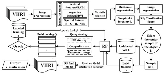
Figure 3.
Overall workflow of the proposed AL algorithm.
Initial sample part (Step 1):
(1) According to a field investigation and visual interpretation, the initial training set is obtained. The RF has two parameters, and the number of trees is 800. This parameter is determined by 10 cross-validations based on OOB scores, and the other parameters are defaults used to set temporary RF0 values.
Sample expansion part (Steps 2–3):
(2) Train the temporary RF0 with the initial training set , obtain the initial classification map, and segment the VHRRS image with a multi-scale segmentation method.
(3) The segmentation image is projected onto the initial classification image, and multiple pixels in the centers of segmentation objects are selected as the expanded sample set , where .
Divide the dataset and set the parameters (Step 4):
(4) In this section, dataset L is divided into two parts: 70% for training and 30% for testing. Then, from the training data, 20 samples are randomly selected for label training (), which includes two parts: class labels and the feature vector. Then, the remaining samples are treated as an unlabeled pool (U), and other samples form a feature vector. In the AL selection iteration, the parameter BATCH-SIZE is used to control the number of samples that need to be labeled by the oracle in each iteration. Referring to related studies, 10 was selected as the BATCH-SIZE [79,80].
AL part (Steps 5–8):
(5) Train an RF based on training label set , use the RF to classify the samples in U, and obtain the probability that each sample belongs to each class. Then, compute the least-confident uncertainty scores by using Equation (3). The similarity scores are calculated according to Algorithm 3 (SID function).
(6) Use the combined query strategy SIDLC to calculate the final score and rank. Algorithm 2 is used to select 10 samples from set U for oracle labeling. The labeled samples form a set l.
(7) Let and , and use to retrain each tree in the RF.
(8) Repeat steps 5 to 8 multiple times; when U = φ or the model reaches the predetermined accuracy criterion, the algorithm stops, and the final RF model is obtained.
3. Experimental Results and Analysis
3.1. Feature Importance Screening Results
The variation in the OOB error with the number of variables calculated by the RFCV method is shown in Figure 4. The most prominent finding is that with the decreasing variables, the OOB score gradually decreases. When the number of variables is greater than 25, changes in the curve tend to be stable. Therefore, 25 features are selected from 210 features to extract the VHRRS urban land use information.
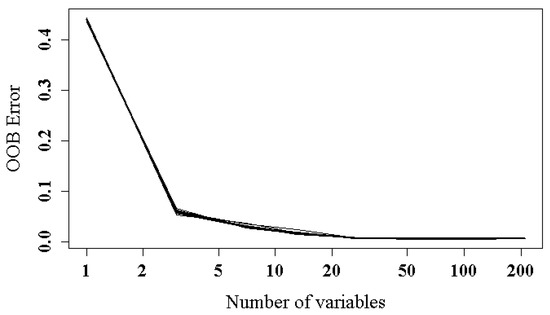
Figure 4.
Effect of the number of variables on OOB error obtained by RFCV for feature selection with all 210 features.
For different land use types, permutation algorithms can be employed to evaluate and rank all 210 features in variable importance. A total of 25 variables are selected for further investigation based on the decrease in accuracy for every urban land use type and mean decrease accuracy (MDA) over all classes (Figure 5). The texture is an important feature for extracting forests and grasslands. For forests, SEC_NIR_13 has the highest importance score, followed by COR_R_13, and for grassland, the red band has the highest MEA_R_13 importance score, followed by MEA_R_5. The NIR-band and GLI are important features that affect information extraction for built-up land. The vegetation index is an important feature for water and barren land. For water, the importance scores of the GNDVI and SAVI are high, and the importance scores of VIgreen and TVI for barren land are high. MEA_G_3 and MEA_G_5 are the most important features for shadow extraction.
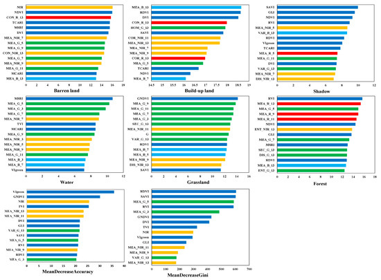
Figure 5.
Variable importance scores of top 15 features. Variable names are given as (feature name)-(base spectral band)-(window size). For example, MEA_NIR_13 indicates an MEA based on an NIR band with a window size of 13 × 13. Bar color indicates the spectral bands, where green band is in green, red band in red, blue band in blue, NIR band in orange, and vegetation index variables in dark blue.
In summary, the features related to the R-band, G-band, and NIR-band correspond to higher importance scores than other features, and the larger the texture calculation window is, the higher the proportion. The results demonstrate that texture features and vegetation indices are important features in extracting VHRRS urban land use information. Therefore, this study selects the top 25 most important feature variables based on MDA as input variables for further analysis (Table 4).

Table 4.
Top 25 features.
3.2. Results of Urban Land Use Information Extraction Based on RBSIDLC
Figure 6a shows the urban land use classification result extracted with the RBSIDLC method, and Table 5 shows the classification accuracy evaluation. Notably, the accuracy of each extracted land use type is greater than 90%, and the overall accuracy (OA) is greater than 96%, indicating that the method based on the RBSIDLC can extract land use information with high accuracy.
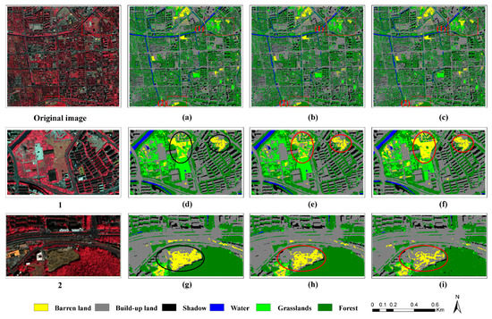
Figure 6.
Classification diagram based on preferred features: (a) RBSIDLC; (b) RBMAL; (c) RF. And two subsets classification diagram (Subset (1) and Subset (2)). Subset (1): (d) RBSIDLC; (e) RBMAL; (f) RF. Subset (2): (g) RBSIDLC; (h) RBMAL; (i) RF.

Table 5.
Class-specific and OA results of the three methods for “preferred features”. The values in this table correspond to the classification results in Figure 6.
As shown in Table 5, RBSIDLC urban land use information extraction yields the highest OA values (96.83%). Compared with the RBMAL and RF methods, the OA is improved by 2.99% and 2.48%, respectively. Compared with the RBMAL method, the RBSIDLC method improves the OAs of barren land, built-up land, water, grassland, and forest; thus, RBSIDLC yields land use extraction results with high accuracy. Compared with the RF algorithm, the RBSIDLC method yields higher OAs for land uses other than water, with improvements to varying degrees. For example, the extraction accuracy of forest increases by approximately 3%, that of grassland increases by approximately 5%, and that of barren land increases by 7%.
The analysis in Table 5 also shows that the OA values of the RF and RBMAL are above 90%. As an estimator of the uncertainty score, the results demonstrate that the RF lays an essential foundation for the extraction of VHRRS urban land use information. Moreover, the SID is used instead of the Euclidean distance in the RBMAL algorithm, which improves the accuracy of the RBSIDLC method and indicates that the similarity function based on the SID is superior to that based on the Euclidean distance.
Figure 6 compares the land use classification results of the RBSIDLC, RBMAL, and RF methods. Further analysis shows that the RBMAL and RF methods seriously confuse barren land and grassland areas (Figure 6e,f, red circle), while the RBSIDLC algorithm can properly distinguish them (Figure 6d, black circle). In addition, the RF algorithm mistakenly classifies barren land as built-up land (Figure 6i, red circle). Although the RBMAL method properly classifies barren land (Figure 6h,i, red circle), the classification result is still inferior to that of RBSIDLC (Figure 6g, black circle).
Overall, these results suggest that the proposed RBSIDLC approach has high accuracy and can effectively classify barren land, grassland, and built-up land compared to the RBMAL and RF algorithms, thus improving the identification accuracy of land use categories and the extraction of urban land use information from VHRRS images. Thus, this method has obvious advantages over traditional methods.
3.3. Comparison with Other AL Query Strategies
In this section, to fully analyze the proposed query strategies, three additional query strategies based on the batch-mode AL method are implemented and used for comparison. The details of BBLC, BBM, and BBE are listed in Table 6. The extraction results for VHRRS urban land use information are shown in Figure 7.

Table 6.
Detailed processes of other query strategies.
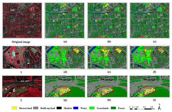
Figure 7.
Optical classification results of the three AL methods when the “preferred feature” combination was used: (a) BBLC; (b) BBM; (c) BBE. And two subsets classification diagram (Subset (1) and Subset (2)). Subset (1): (d) BBLC; (e) BBM; (f) BBE. Subset (2): (g) BBLC; (h) BBM; (i) BBE.
It is apparent that the BBLC, BBM, and BBE methods seriously confuse barren land and built-up land (Figure 7d–f, red circle). In the BBLC and BBE algorithms, an extreme situation occurs in which barren land is misclassified as built-up land and grassland, especially in the BBLC algorithm; moreover, many barren land areas are misclassified as built-up land (Figure 7d, red circle). Although the BBM algorithm corrects the error, it still incorrectly classifies grassland as barren land. The RBSIDLC algorithm can properly identify grassland, barren land, and built-up land areas, and the classification result is the best among the results of the considered methods (Figure 6d, black circle).
Thus, a single query with a high number of samples increases the risk of confusion when querying samples (Figure 7d,f, red circle). The RBMAL algorithm mitigates this phenomenon by ranking samples based on the amount of information (Figure 6e, red circle), and RBSIDLC inherits the advantages of the RBMAL algorithm and replaces the Euclidean distance in the similarity function with the SID to further improve the accuracy of recognition for each category (Figure 6d,g, black circle). This approach has obvious advantages in urban land use classification.
Figure 8 shows the OA of urban land use information extraction, and the results of the RF, RBMAL, and RBSIDLC methods are compared with those of the methods in Table 6. The accuracies of BBLC and BBE are lower than that of the RF by 2.49% and 4.71%, respectively. Compared with that of the RF, the accuracy of the BBM algorithm is only 0.85% higher. This demonstrates that algorithms based on the batch-mode AL method may reduce the accuracy of RFs while increasing the number of labeled samples in a parallel environment. The accuracy of the RBMAL algorithm is 3% and 5.22% higher than the accuracies of the BBLC and BBE algorithms, respectively, which indicates that the combined query strategy is more effective than single query strategies. The SID is used to replace the Euclidean distance in the similarity measurement function used in the RBMAL algorithm. The constructed RBSIDLC combined query strategy further improves urban land use classification accuracy, with the highest accuracy reaching 96.83%.
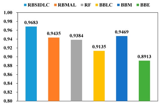
Figure 8.
OAs of the preferred feature classification results with different algorithms.
Figure 9 shows a confusion matrix that was used to further analyze the three AL methods in Table 6 and the results of urban land use information extraction with the RF, RBMAL, and RBSIDLC.
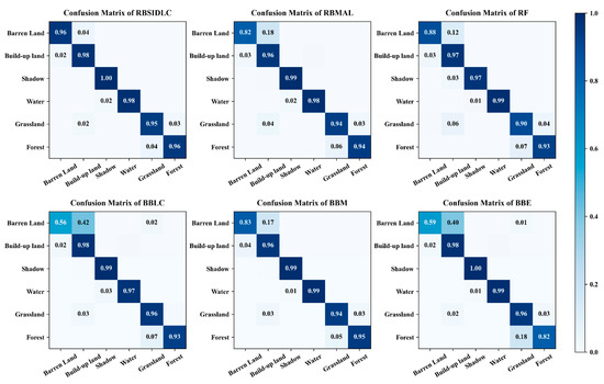
Figure 9.
Confusion matrix of the classification results of six algorithms based on preferred features.
The RBMAL and RF misclassify 18% and 12% of barren land as built-up land, respectively, and 4% and 6% of grassland as built-up land, respectively (Figure 9). In contrast, the RBSIDLC algorithm reduces the misclassification to 4% between barren land and built-up land and 2% between grassland and built-up land. Therefore, the RBSIDLC method outperforms the other methods. Further analysis showed that the BBLC, BBM, and BBE algorithms mistakenly divide barren land into built-up land. The single most striking observation from the figure comparison is that the BBLC and BBE algorithms commonly misclassify barren land as built-up land and grassland. For example, the BBLC and BBE algorithms mistakenly classify 42% and 40% of barren land as built-up land, and 2% and 1% of barren land is misclassified as grassland, respectively. Compared with the BBLC, BBM, and BBE methods, the RBSIDLC algorithm improves the barren land, built-up land, and grassland classifications to varying degrees. For example, compared with that of the BBE algorithm, the barren land extraction accuracy of the RBSIDLC algorithm is increased by 37%, and the vegetation extraction accuracy is increased by 14%.
Together, the results confirm that each query strategy struggles to distinguish between barren land, grassland, and built-up land features. RBMAL can correctly identify most of the features by combining query strategies and RBSIDLC replaces Euclidean distance with the SID to obtain an improved classification result, indicating that a similarity function based on the SID is a better one based on Euclidean distance.
The sample labeling cost is an important index used to evaluate AL. In this study, referring to the relevant literature, we set the RF accuracy threshold and obtain the number of samples required by different AL algorithms. Then, all the methods in our experiments were implemented using Visual Studio Code platform python 3.7 with 3.7 GHz Intel i9-10900K CPU and 32 GB RAM. The SavedRate of different query strategies is then calculated [81] (Table 7).

Table 7.
Cost evaluation of five active learning methods with labeling.
The results indicate that the three query strategies based on the BBLC, BBM, and BBE methods require the most samples, followed by RBMAL, with RBSIDLC ranking last, which means that RBSIDLC is associated with the lowest sample labeling cost (Table 7). This result demonstrates that the proposed query strategy achieves the expected effect with as low an annotation cost as possible, accelerates the labeling of samples per unit time, and improves efficiency.
4. Discussion
The RBSIDLC method proposed in this study achieves high accuracy levels in the extraction of urban land use information from VHRRS images. Compared with other batch-mode AL query strategies, this method yields the highest accuracy, with an OA of 96.83%. These superior results can be explained from the following three perspectives.
First, an RF was adopted to estimate the uncertainty score in the SIDLC combined query strategy. Uncertainty estimation is the process of estimating the informativeness of an unlabeled sample. The labeled samples are added to the training set and the RF is used as a classifier to retrain the model for the next estimation. This cycle improves the estimator’s performance and the training accuracy of the RF, thus providing an important foundation for the extraction of VHRRS urban land use information. In addition, the SID is used to replace the Euclidean distance in the RBMAL algorithm, and the spectral and spatial characteristics of VHRRS images are fully considered, which effectively solves the misclassification issues for barren land, grassland, and built-up land observed for the RBMAL and RF algorithms, thereby improving the precision of land use category identification.
Moreover, the query strategy has a considerable impact on the accuracy of batch-mode AL information extraction. This study analyzes the OAs of different query strategies and RBSIDLC in extracting urban land use information (Figure 8). The BBLC, BBM, and BBE methods use a single query strategy to query many samples at a time, which increases the risk that confusion among query samples will affect the accuracy of the classifier (Figure 9 and Figure 10). Although the RBMAL algorithm mitigates this phenomenon, the information extraction results are still not ideal (Figure 7e). By inheriting the advantages of the RBMAL algorithm, RBSIDLC adopts the SIDLC combined query strategy, which improves the recognition rate of each category and yields the highest accuracy in urban land use information extraction. These results support the hypothesis that the SIDLC combined query strategy is more effective than a single query strategy.
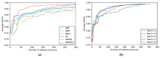
Figure 10.
Iterative querying of preferred features: (a) training accuracy; (b) effects of the batch size in the proposed AL algorithm on preferred feature results.
Finally, the labeling quality of training samples is high for RBSIDLC to achieve VHRRS urban land use information. Figure 10a shows the training accuracy curves of all the compared algorithms based on preferred features. It is apparent from this figure that as the number of labeled samples increases, the changes in accuracy for RBMAL and RBSIDLC become more stable than those of the other methods; notably, RBSIDLC displays no apparent fluctuations. Further analysis showed that the RBSIDLC algorithm can query and obtain high-quality training samples. However, the results of the BBLC, BBM, and BBE algorithms fluctuate broadly, especially in the range of 0–100, which indicates that the training samples they query are chaotic. The results show clearly that RBSIDLC can select high-quality samples and reduce disturbances in the batch-mode AL method, thereby ensuring the accuracy of land use information extraction.
The parameter BATCH-SIZE in the iterative AL selection process is used to control the number of samples that need to be labeled by the oracle in each iteration. In this study, referring to relevant studies, we set BATCH-SIZE to 10 and achieved promising results. Additionally, the effect of BATCH-SIZE (set to 1, 3, 5, 7, and 9) on the accuracy is assessed, as shown in Figure 10b. The most prominent finding is that with increasing BATCH-SIZE, the model’s accuracy is improved, and the fluctuations in batch processing are reduced. The results of this study indicate that it is reasonable to adopt a value of 10 for BATCH-SIZE.
In addition, this paper uses the permutation method to rank the feature importance of all variables and selects 25 features from 210 feature variables to be included in the extraction of urban land use information. The results are improved with this approach. We further explored the importance of each feature for sample separation and selected nine important features for analysis. The results indicate that vegetation (forest and grassland) displays strong reflection in the NIR-band and for the vegetation indices, namely the TVI, DVI, and GNDVI (Figure 11). Forests and grasslands can have high reflection values based on different vegetation types. For VIgreen, GLI, MEA_G_5, and MEA_R_13, the six land use categories exhibit a favorable gradient distribution, and the average of each category is highly variable.
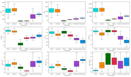
Figure 11.
Preferred feature index. The centerline in each box in the boxplot is the median, and the edges of the box represent the upper and lower quartiles. Spectral characteristics: NIR; vegetation indexes: GLI, GNDVI, TVI, DVI, and VIgreen; texture feature: MEA_G_5, MEA_R_13, and SEC_NIR_13.
Further analysis shows that the selected features yield a good degree of separation for the six land use categories. This preliminary finding suggests that the proposed feature selection method outperforms most artificial feature combination methods.
Based on this research, there is a lot of work to be carried out in the future. First, we can further study the two parts of the query function: (1) other similarity functions can be considered, such as distance-based spectral similarity measurement method, spectral angle similarity measurement, etc.; (2) in the uncertainty estimation part, the combinations of different classifiers and uncertainty strategy will produce different results, and we can replace the base classifier, for example, KNN, SVM, etc. We can also choose different query strategies to find the best combination for remote sensing image information extraction. In addition, deep learning is an effective tool for dealing with complex classification problems. How to use deep learning models to improve the ability of active learning algorithms is also worth studying.
5. Conclusions
This paper proposes a ranked batch-mode AL classification framework with a new query strategy called SIDLC for improving the accuracy in extracting urban land use information from VHRRS images. For the optimal feature dataset, the OA of RF classification are both above 90% for the proposed method. As the estimator of uncertainty scores and the core classifier used in the framework, the RF lays the foundation for the high-precision extraction of VHRRS urban land use information. The RBSIDLC algorithm replaces the Euclidean distance in the RBMAL algorithm with the SID. Due to the advantages of RBMAL, the spectral and spatial information in VHRRS images is fully analyzed; notably, the classification OA reaches 96.83%. These experiments confirm that replacing the Euclidean distance with the SID in the similarity function can improve extraction performance. In addition, the SIDLC combined query strategy performs better than the batch-mode AL single query strategies, and the misclassification rates among different land types are reduced. Compared to the BBE algorithm, the extraction accuracy of barren land for the RBSIDLC algorithm increases by 37%, and the accuracy of vegetation extraction increases by 14%. This study finds that the SIDLC-based RBSIDLC algorithm has obvious advantages in extracting urban land use information from VHRRS images. Additionally, the Worldview-3 image is an important basis for feature extraction, and has great potential in urban land use information extraction. The RF feature selection method is used to select the optimal features for classification, thus avoiding subjective influence and dimensionality issues and improving model performance. The proposed approach provides a reference for selecting the optimal features and extracting VHRRS urban land use information. There is a lot of future work. Firstly, the two main components of combined query strategies could be further investigated. Secondly, how to use deep learning models to improve the ability of AL algorithms is also worth studying. Finally, studying the best components of the solution in remote sensing image information extraction will bring completely new challenges.
Author Contributions
Conceptualization, X.L. (Xin Luo) and H.D.; Data curation, X.L. (Xin Luo), X.L. (Xuejian Li), D.Z., Y.X., M.Z., S.H. and Z.H.; Formal analysis, X.L. (Xin Luo), X.L. (Xuejian Li), F.M., D.Z., Y.X., M.Z. and S.H.; Funding acquisition, H.D. and G.Z.; Investigation, X.L. (Xin Luo); Methodology, X.L. (Xin Luo); Project administration, H.D.; Software, X.L. (Xin Luo) and Z.H.; Validation, X.L. (Xin Luo) and S.H.; Visualization, X.L. (Xin Luo); Writing—original draft, X.L. (Xin Luo); Writing—review and editing, H.D. All authors have read and agreed to the published version of the manuscript.
Funding
This research was funded by the National Natural Science Foundation (No. U1809208, No. 31901310, No. 31800538), the State Key Laboratory of Subtropical Silviculture (No. ZY20180201), the Key Research and Development Program of Zhejiang Province (2021C02005).
Institutional Review Board Statement
Not applicable.
Informed Consent Statement
Not applicable.
Acknowledgments
The authors gratefully acknowledge the supports of various foundations. The authors are grateful to the editor and anonymous reviewers whose comments have contributed to improving the quality.
Conflicts of Interest
The authors declare that they have no competing interest.
References
- Li, M.; Stein, A.; Bijker, W.; Zhan, Q. Urban land use extraction from Very High Resolution remote sensing imagery using a Bayesian network. ISPRS J. Photogramm. Remote Sens. 2016, 122, 192–205. [Google Scholar] [CrossRef]
- Huang, X.; Wang, Y. Investigating the effects of 3D urban morphology on the surface urban heat island effect in urban functional zones by using high-resolution remote sensing data: A case study of Wuhan, Central China. ISPRS J. Photogramm. Remote Sens. 2019, 152, 119–131. [Google Scholar] [CrossRef]
- Cao, R.; Tu, W.; Yang, C.; Li, Q.; Liu, J.; Zhu, J.; Zhang, Q.; Li, Q.; Qiu, G. Deep learning-based remote and social sensing data fusion for urban region function recognition. ISPRS J. Photogramm. Remote Sens. 2020, 163, 82–97. [Google Scholar] [CrossRef]
- Zhou, M.; Sui, H.; Chen, S.; Wang, J.; Chen, X. BT-RoadNet: A boundary and topologically-aware neural network for road extraction from high-resolution remote sensing imagery. ISPRS J. Photogramm. Remote Sens. 2020, 168, 288–306. [Google Scholar] [CrossRef]
- Fang, F.; McNeil, B.E.; Warner, T.A.; Maxwell, A.E.; Dahle, G.A.; Eutsler, E.; Li, J. Discriminating tree species at different taxonomic levels using multi-temporal Worldview-3 imagery in Washington, DC, USA. Remote Sens. Environ. 2020, 246, 111811. [Google Scholar] [CrossRef]
- Chen, M.; Wu, J.; Liu, L.; Zhao, W.; Tian, F.; Shen, Q.; Zhao, B.; Du, R. DR-Net: An improved network for building extraction from high resolution remote sensing image. Remote Sens. 2021, 13, 294. [Google Scholar] [CrossRef]
- Geiß, C.; Aravena Pelizari, P.; Blickensdörfer, L.; Taubenböck, H. Virtual support vector machines with self-learning strategy for classification of multispectral remote sensing imagery. ISPRS J. Photogramm. Remote Sens. 2019, 151, 42–58. [Google Scholar] [CrossRef]
- Dabija, A.; Kluczek, M.; Zagajewski, B.; Raczko, E.; Kycko, M.; Al-Sulttani, A.H.; Tardà, A.; Pineda, L.; Corbera, J. Comparison of support vector machines and random forests for corine land cover mapping. Remote Sens. 2021, 13, 777. [Google Scholar] [CrossRef]
- Cui, L.; Du, H.; Zhou, G.; Li, X.; Mao, F.; Xu, X.; Fan, W.; Li, Y.; Zhu, D.; Liu, T.; et al. Combination of decision tree and mixed pixel decomposition for extracting bamboo forest information in China. Yaogan Xuebao J. Remote Sens. 2019, 23, 166–176. [Google Scholar] [CrossRef]
- Dong, L.; Xing, L.; Liu, T.; Du, H.; Mao, F.; Han, N.; Li, X.; Zhou, G.; Zhu, D.; Zheng, J.; et al. Very high resolution remote sensing imagery classification using a fusion of random forest and deep learning technique—Subtropical area for example. IEEE J. Sel. Top. Appl. Earth Obs. Remote Sens. 2020, 13, 113–128. [Google Scholar] [CrossRef]
- Belgiu, M.; Drăgu, L. Random forest in remote sensing: A review of applications and future directions. ISPRS J. Photogramm. Remote Sens. 2016, 114, 24–31. [Google Scholar] [CrossRef]
- Paoletti, M.E.; Haut, J.M.; Plaza, J.; Plaza, A. Deep learning classifiers for hyperspectral imaging: A review. ISPRS J. Photogramm. Remote Sens. 2019, 158, 279–317. [Google Scholar] [CrossRef]
- He, S.; Du, H.; Zhou, G.; Li, X.; Mao, F.; Zhu, D.; Xu, Y.; Zhang, M.; Huang, Z.; Liu, H.; et al. Intelligent mapping of urban forests from high-resolution remotely sensed imagery using object-based u-net-densenet-coupled network. Remote Sens. 2020, 12, 3928. [Google Scholar] [CrossRef]
- Ma, L.; Liu, Y.; Zhang, X.; Ye, Y.; Yin, G.; Johnson, B.A. Deep learning in remote sensing applications: A meta-analysis and review. ISPRS J. Photogramm. Remote Sens. 2019, 152, 166–177. [Google Scholar] [CrossRef]
- Zhang, L.; Zhang, Q.; Zhang, L.; Tao, D.; Huang, X.; Du, B. Ensemble manifold regularized sparse low-rank approximation for multiview feature embedding. Pattern Recognit. 2015, 48, 3102–3112. [Google Scholar] [CrossRef]
- Xia, J.; Liao, W.; Chanussot, J.; Du, P.; Song, G.; Philips, W. Improving random forest with ensemble of features and semisupervised feature extraction. IEEE Geosci. Remote Sens. Lett. 2015, 12, 1471–1475. [Google Scholar] [CrossRef]
- Zhang, Y.; Zong, R.; Han, J.; Zheng, H.; Lou, Q.; Zhang, D.; Wang, D. TransLand: An adversarial transfer learning approach for migratable urban land usage classification using remote sensing. In Proceedings of the 2019 IEEE International Conference on Big Data, Los Angeles, CA, USA, 9–12 December 2019; pp. 1567–1576. [Google Scholar]
- Sun, X.; Wang, B.; Wang, Z.; Li, H.; Li, H.C.; Fu, K. Research progress on few-shot learning for remote sensing image interpretation. IEEE J. Sel. Top. Appl. Earth Obs. Remote Sens. 2021. [Google Scholar] [CrossRef]
- Zhu, X. Semi-Supervised Learning Literature Survey; University of Wisconsin-Madison Department of Computer Sciences, College of Letters and Science, University of Wisconsin–Madison, 2006; Volume 2, pp. 607–608. Available online: https://minds.wisconsin.edu/handle/1793/60444 (accessed on 1 June 2021).
- Kong, Y.; Wang, X.; Cheng, Y.; Chen, C.L.P. Hyperspectral imagery classification based on semi-supervised broad learning system. Remote Sens. 2018, 10, 685. [Google Scholar] [CrossRef]
- Shi, C.; Lv, Z.; Yang, X.; Xu, P.; Bibi, I. Hierarchical multi-view semi-supervised learning for very high-resolution remote sensing image classification. Remote Sens. 2020, 12, 1012. [Google Scholar] [CrossRef]
- Xia, G.-S.; Wang, Z.; Xiong, C.; Zhang, L. Accurate annotation of remote sensing images via active spectral clustering with little expert knowledge. Remote Sens. 2015, 7, 15014–15045. [Google Scholar] [CrossRef]
- Demarchi, L.; Canters, F.; Cariou, C.; Licciardi, G.; Chan, J.C.W. Assessing the performance of two unsupervised dimensionality reduction techniques on hyperspectral APEX data for high resolution urban land-cover mapping. ISPRS J. Photogramm. Remote Sens. 2014, 87, 166–179. [Google Scholar] [CrossRef]
- Sheikholeslami, M.M.; Nadi, S.; Naeini, A.A.; Ghamisi, P. An efficient deep unsupervised superresolution model for remote sensing images. IEEE J. Sel. Top. Appl. Earth Obs. Remote Sens. 2020, 13, 1937–1945. [Google Scholar] [CrossRef]
- Wang, S.; Chen, W.; Xie, S.M.; Azzari, G.; Lobell, D.B. Weakly supervised deep learning for segmentation of remote sensing imagery. Remote Sens. 2020, 12, 207. [Google Scholar] [CrossRef]
- Zhang, W.; Tang, P.; Corpetti, T.; Zhao, L. WTS: A Weakly towards strongly supervised learning framework for remote sensing land cover classification using segmentation models. Remote Sens. 2021, 13, 394. [Google Scholar] [CrossRef]
- Tuia, D.; Ratle, F.; Pacifici, F.; Kanevski, M.F.; Emery, W.J. Active learning methods for remote sensing image classification. IEEE Trans. Geosci. Remote Sens. 2009, 47, 2218–2232. [Google Scholar] [CrossRef]
- Tuia, D.; Pasolli, E.; Emery, W.J. Using active learning to adapt remote sensing image classifiers. Remote Sens. Environ. 2011, 115, 2232–2242. [Google Scholar] [CrossRef]
- Settles, B. Active Learning. Synthesis Lectures on Artificial Intelligence and Machine Learning. 2012, pp. 1–114. Available online: https://www.morganclaypool.com/doi/abs/10.2200/S00429ED1V01Y201207AIM018 (accessed on 1 March 2021). [CrossRef]
- Li, J.; Huang, X.; Chang, X. A label-noise robust active learning sample collection method for multi-temporal urban land-cover classification and change analysis. ISPRS J. Photogramm. Remote Sens. 2020, 163, 1–17. [Google Scholar] [CrossRef]
- Stumpf, A.; Lachiche, N.; Malet, J.P.; Kerle, N.; Puissant, A. Active learning in the spatial domain for remote sensing image classification. IEEE Trans. Geosci. Remote Sens. 2014, 52, 2492–2507. [Google Scholar] [CrossRef]
- Ma, K.Y.; Chang, C.-I. Iterative training sampling coupled with active learning for semisupervised spectral-spatial hyperspectral image classification. IEEE Trans. Geosci. Remote Sens. 2021, 1–21. [Google Scholar] [CrossRef]
- Han, W.; Coutinho, E.; Ruan, H.; Li, H.; Schuller, B.; Yu, X.; Zhu, X. Semi-supervised active learning for sound classification in hybrid learning environments. PLoS ONE 2016, 11. [Google Scholar] [CrossRef]
- Haertel, R.; Felt, P.; Ringger, E.; Seppi, K. Parallel active learning: Eliminating wait time with minimal staleness. In Proceedings of the NAACL HLT 2010 Workshop on Active Learning for Natural Language Processing, Department of Computer ScienceBrigham Young University, Provo, UT, USA, 1 June 2010. [Google Scholar]
- Demir, B.; Persello, C.; Bruzzone, L. Batch-mode active-learning methods for the interactive classification of remote sensing images. IEEE Trans. Geosci. Remote Sens. 2011, 49, 1014–1031. [Google Scholar] [CrossRef]
- Shi, L.; Zhao, Y.; Tang, J. Batch mode active learning for networked data. ACM Trans. Intell. Syst. Technol. 2012, 3, 1–25. [Google Scholar] [CrossRef]
- Shi, Q.; Du, B.; Zhang, L. Spatial coherence-based batch-mode active learning for remote sensing image classification. IEEE Trans. Image Process. 2015, 24, 2037–2050. [Google Scholar] [CrossRef]
- Cardoso, T.N.; Silva, R.M.; Canuto, S.; Moro, M.M.; Gonçalves, M.A. Ranked batch-mode active learning. Inform. Sci. 2017, 379, 313–337. [Google Scholar] [CrossRef]
- Qu, Z.; Du, J.; Cao, Y.; Guan, Q.; Zhao, P. Deep active learning for remote sensing object detection. arXiv 2020, arXiv:2003.08793. [Google Scholar]
- Balcan, M.F.; Broder, A.Z.; Zhang, T. Margin based active learning. In Proceedings of the Conference on Learning Theory, San Diego, CA, USA, 13–15 June 2007; pp. 35–50. [Google Scholar]
- Kumari, P.; Chaudhuri, S.; Borkar, V.; Chaudhuri, S. Maximizing Conditional Entropy for Batch-Mode Active Learning of Perceptual Metrics. 2021. Available online: http://arxiv.org/abs/2102.07365 (accessed on 17 March 2021).
- Dasgupta, S. Two faces of active learning. Theor. Comput. Sci. 2011, 412, 1767–1781. [Google Scholar] [CrossRef]
- Shui, C.; Zhou, F.; Gagné, C.; Wang, B. Deep active learning: Unified and principled method for query and training. arXiv 2019, arXiv:1911.09162. [Google Scholar]
- Ji, X.; Cui, Y.; Teng, L. Joint multi-mode cooperative classification algorithm for hyperspectral images. J. Appl. Remote Sens. 2021, 15, 1–25. [Google Scholar] [CrossRef]
- Yan, S.; Jing, L.; Wang, H. A new individual tree species recognition method based on a convolutional neural network and high-spatial resolution remote sensing imagery. Remote Sens. 2021, 13, 479. [Google Scholar] [CrossRef]
- Maurer, T. How to pan-sharpen images using the gram-schmidt pan-sharpen method—A recipe. ISPRS Int. Arch. Photogramm. Remote Sens. Spat. Inf. Sci. 2013, XL-1/W1, 239–244. [Google Scholar] [CrossRef]
- Anderson, J.R.; Hardy, E.E.; Roach, J.T.; Witmer, R.E. A Land Use and Land Cover Classification System for Use with Remote Sensor Data; USGS Professional Paper, No. 964; US Government Printing Office: Washington, DC, USA, 1976. [CrossRef]
- Sun, J.; Wang, H.; Song, Z.; Lu, J.; Meng, P.; Qin, S. Mapping essential urban land use categories in nanjing by integrating multi-source big data. Remote Sens. 2020, 12, 2386. [Google Scholar] [CrossRef]
- Gong, P.; Liu, H.; Zhang, M.; Li, C.; Wang, J.; Huang, H.; Clinton, N.; Ji, L.; Li, W.; Bai, Y.; et al. Stable classification with limited sample: Transferring a 30-m resolution sample set collected in 2015 to mapping 10-m resolution global land cover in 2017. Sci. Bull. 2019, 64, 370–373. [Google Scholar] [CrossRef]
- Shahi, K.; Shafri, H.Z.M.; Taherzadeh, E.; Area, A.S. A Novel Spectral Index for Automatic Shadow Detection in Urban Mapping Based On WorldView-2 Satellite Imagery. 2014. Available online: https://waset.org/publications/9999443/a-novel-spectral-index-for-automatic-shadow-detection-in-urban-mapping-based-on-worldview-2-satellite-imagery (accessed on 3 June 2021).
- Dare, P.M. Shadow analysis in high-resolution satellite imagery of urban areas. Photogramm. Eng. Remote Sens. 2005, 71, 169–177. [Google Scholar] [CrossRef]
- Fatiha, B.; Abdelkader, A.; Latifa, H.; Mohamed, E. Spatio temporal analysis of vegetation by vegetation indices from multi-dates satellite images: Application to a semi arid area in ALGERIA. Energy Procedia 2013, 36, 667–675. [Google Scholar] [CrossRef]
- Li, Y.; Han, N.; Li, X.; Du, H.; Mao, F.; Cui, L.; Liu, T.; Xing, L. Spatiotemporal estimation of bamboo forest aboveground carbon storage based on Landsat data in Zhejiang, China. Remote Sens. 2018, 10, 898. [Google Scholar] [CrossRef]
- Xu, K.; Qian, J.; Hu, Z.; Duan, Z.; Chen, C.; Liu, J.; Sun, J.; Wei, S.; Xing, X. A new machine learning approach in detecting the oil palm plantations using remote sensing data. Remote Sens. 2021, 13, 236. [Google Scholar] [CrossRef]
- Zhang, M.; Du, H.; Zhou, G.; Li, X.; Mao, F.; Dong, L.; Zheng, J.; Liu, H.; Huang, Z.; He, S. Estimating forest aboveground carbon storage in Hang-Jia-Hu using landsat TM/OLI data and random forest model. Forests 2019, 10, 1004. [Google Scholar] [CrossRef]
- Gao, G.; Du, H.; Han, N.; Xu, X.; Sun, S.; Li, X. Mapping of moso bamboo forest using object-based approach based on the optimal features. Scientia Silvae Sinicae 2016, 52, 77–85. [Google Scholar] [CrossRef]
- Jordan, C.F. Derivation of leaf-area index from quality of light on the forest floor. Ecology 1969, 50, 663–666. [Google Scholar] [CrossRef]
- Ren, H.; Zhou, G.; Zhang, F. Using negative soil adjustment factor in soil-adjusted vegetation index (SAVI) for aboveground living biomass estimation in arid grasslands. Remote Sens. Environ. 2018, 209, 439–445. [Google Scholar] [CrossRef]
- Tucker, C.J. Red and photographic infrared linear combinations for monitoring vegetation. Remote Sens. Environ. 1979, 8, 127–150. [Google Scholar] [CrossRef]
- Gitelson, A.A.; Merzlyak, M.N. Remote sensing of chlorophyll concentration in higher plant leaves. Adv. Space Res. 1998, 22, 689–692. [Google Scholar] [CrossRef]
- Huete, A.R. A soil-adjusted vegetation index (SAVI). Remote Sens. Environ. 1988, 25, 295–309. [Google Scholar] [CrossRef]
- Karlson, M.; Ostwald, M.; Reese, H.; Bazié, H.R.; Tankoano, B. Assessing the potential of multi-seasonal WorldView-2 imagery for mapping West African agroforestry tree species. Int. J. Appl. Earth Obs. Geoinf. 2016, 50, 80–88. [Google Scholar] [CrossRef]
- Dash, J.; Curran, P.J. The MERIS terrestrial chlorophyll index. Int. J. Remote Sens. 2004, 25, 5403–5413. [Google Scholar] [CrossRef]
- Haboudane, D.; Miller, J.R.; Pattey, E.; Zarco-Tejada, P.J.; Strachan, I.B. Hyperspectral vegetation indices and novel algorithms for predicting green LAI of crop canopies: Modeling and validation in the context of precision agriculture. Remote Sens. Environ. 2004, 90, 337–352. [Google Scholar] [CrossRef]
- Haboudane, D.; Tremblay, N.; Miller, J.R.; Vigneault, P. Using Spectral Indices Derived From Hyperspectral Data. IEEE Geosci. Remote. Sens. 2008, 46, 423–437. [Google Scholar] [CrossRef]
- Roujean, J.L.; Breon, F.M. Estimating PAR absorbed by vegetation from bidirectional reflectance measurements. Remote Sens. Environ. 1995, 51, 375–384. [Google Scholar] [CrossRef]
- Gitelson, A.A. Remote estimation of canopy chlorophyll content in crops. Geophys. Res. Lett. 2005, 32, L08403. [Google Scholar] [CrossRef]
- Louhaichi, M.; Borman, M.M.; Johnson, D.E. Spatially located platform and aerial photography for documentation of grazing impacts on wheat. Geocarto Int. 2001, 16, 65–70. [Google Scholar] [CrossRef]
- Huete, A.; Didan, K.; Miura, T.; Rodriguez, E.P.; Gao, X.; Ferreira, L.G. Overview of the radiometric and biophysical performance of the MODIS vegetation indices. Remote Sens. Environ. 2002, 83, 195–213. [Google Scholar] [CrossRef]
- Haralick, R.M.; Dinstein, I.; Shanmugam, K. Textural features for image classification. IEEE Trans. Syst. Man Cybern. 1973, SMC-3, 610–621. [Google Scholar] [CrossRef]
- Li, X.; Du, H.; Mao, F.; Zhou, G.; Chen, L.; Xing, L.; Fan, W.; Xu, X.; Liu, Y.; Cui, L.; et al. Estimating bamboo forest aboveground biomass using EnKF-assimilated MODIS LAI spatiotemporal data and machine learning algorithms. Agric. For. Meteorol. 2018, 256, 445–457. [Google Scholar] [CrossRef]
- Van der Meer, F. The effectiveness of spectral similarity measures for the analysis of hyperspectral imagery. Int. J. Appl. Earth Obs. Geoinf. 2006, 8, 3–17. [Google Scholar] [CrossRef]
- Zhang, Y.; Cao, G.; Li, X.; Wang, B.; Fu, P. Active semi-supervised random forest for hyperspectral image classification. Remote Sens. 2019, 11, 2974. [Google Scholar] [CrossRef]
- Zhao, C.; Tian, M.; Li, J. Research progress on spectral similarity metrics. Harbin Gongcheng Daxue Xuebao J. Harbin Eng. Univ. 2017, 38, 1179–1189. [Google Scholar] [CrossRef]
- Chang, C.I. Spectral information divergence for hyperspectral image analysis. In Proceedings of the IEEE International Geoscience and Remote Sensing Symposium (IGARSS 1999), Hamburg, Germany, 28 June–2 July 1999; pp. 509–511. [Google Scholar]
- Chang, C.I. An information-theoretic approach to spectral variability, similarity, and discrimination for hyperspectral image analysis. IEEE Trans. Inf. Theory 2000, 46, 1927–1932. [Google Scholar] [CrossRef]
- Vakil, M.I.; Malas, J.A.; Megherbi, D.B. An information theoretic metric for identifying optimum solution for normalized cross correlation based similarity measures. In Proceedings of the IEEE National Aerospace Electronics Conference, NAECON, Dayton, OH, USA, 15–19 June 2015; Volume 2016, pp. 136–140. [Google Scholar]
- Zhang, E.; Zhang, X.; Yang, S.; Wang, S. Improving hyperspectral image classification using spectral information divergence. IEEE Geosci. Remote Sens. Lett. 2014, 11, 249–253. [Google Scholar] [CrossRef]
- Wan, L.; Tang, K.; Li, M.; Zhong, Y.; Qin, A.K. Collaborative active and semisupervised learning for hyperspectral remote sensing image classification. IEEE Trans. Geosci. Remote Sens. 2015, 53, 2384–2396. [Google Scholar] [CrossRef]
- Wang, Z.; Du, B.; Zhang, L.; Zhang, L.; Jia, X. A novel semisupervised active-learning algorithm for hyperspectral image classification. IEEE Trans. Geosci. Remote Sens. 2017, 55, 3071–3083. [Google Scholar] [CrossRef]
- Hou, C.; Yang, C. Research on Strategies of Active Learning and Its Application to Image Classification. Ph.D. Thesis, Xiamen University, Xiamen, China, 2019. [Google Scholar]
Publisher’s Note: MDPI stays neutral with regard to jurisdictional claims in published maps and institutional affiliations. |
© 2021 by the authors. Licensee MDPI, Basel, Switzerland. This article is an open access article distributed under the terms and conditions of the Creative Commons Attribution (CC BY) license (https://creativecommons.org/licenses/by/4.0/).
