Article

Improved YOLO Network for Free-Angle Remote Sensing Target Detection

School of Instrument and Electronics, North University of China, Taiyuan 030000, China
*
Author to whom correspondence should be addressed.
Remote Sens. 2021, 13(11), 2171; https://doi.org/10.3390/rs13112171
Submission received: 24 April 2021 / Revised: 28 May 2021 / Accepted: 29 May 2021 / Published: 1 June 2021
(This article belongs to the Special Issue Deep Learning and Computer Vision in Remote Sensing)

Abstract

:
Despite significant progress in object detection tasks, remote sensing image target detection is still challenging owing to complex backgrounds, large differences in target sizes, and uneven distribution of rotating objects. In this study, we consider model accuracy, inference speed, and detection of objects at any angle. We also propose a RepVGG-YOLO network using an improved RepVGG model as the backbone feature extraction network, which performs the initial feature extraction from the input image and considers network training accuracy and inference speed. We use an improved feature pyramid network (FPN) and path aggregation network (PANet) to reprocess feature output by the backbone network. The FPN and PANet module integrates feature maps of different layers, combines context information on multiple scales, accumulates multiple features, and strengthens feature information extraction. Finally, to maximize the detection accuracy of objects of all sizes, we use four target detection scales at the network output to enhance feature extraction from small remote sensing target pixels. To solve the angle problem of any object, we improved the loss function for classification using circular smooth label technology, turning the angle regression problem into a classification problem, and increasing the detection accuracy of objects at any angle. We conducted experiments on two public datasets, DOTA and HRSC2016. Our results show the proposed method performs better than previous methods.

Graphical Abstract

1. Introduction

Target detection is a basic task in computer vision and helps estimate the category of objects in a scene and mark their locations. The rapid deployment of airborne and spaceborne sensors has made ultra-high-resolution aerial images common. However, object detection in remote sensing images remains a challenging task. Research on remote sensing images has crucial applications in the military, disaster control, environmental management, and transportation planning [1,2,3,4]. Therefore, it has attracted significant attention from researchers in recent years.
Object detection in aerial images has become a prevalent topic in computer vision [5,6,7]. In the past few years, machine learning methods have been successfully applied for remote sensing target detection [8,9,10]. David et al. [8] used the Defense Science and Technology Organization Analysts’ Detection Support System, which is a system developed particularly for ship detection in remote sensing images. Wang et al. [9] proposed an intensity-space domain constant false alarm rate ship detector. Leng et al. [10] presented a highly adaptive ship detection scheme for spaceborne synthetic-aperture radar (SAR) imagery.
Although these remote sensing target detection methods based on machine learning have achieved good results, the missed detection rate remains very high in complex ground environments. Deep neural networks, particularly the convolutional neural network (CNN) class, significantly improve the detection of objects in natural images owing to the advantages in robust feature extraction using large-scale datasets. In recent years, systems employing the powerful feature learning capabilities of CNN have demonstrated remarkable success in various visual tasks such as classification [11,12], segmentation [13], tracking [14], and detection [15,16,17]. CNN-based target detectors can be divided into two categories: single-stage and two-stage target detection networks. Single-stage target detection networks discussed in the literature [18,19,20,21] include a you only look once (YOLO) detector optimized end-to-end, which was proposed by Joseph et al. [18,19]. Liu et al. [20] presented a method for detecting objects in images using a deep neural network single-shot detector (SSD). Lin et al. [21] designed and trained a simple dense object detector, RetinaNet, to evaluate the effectiveness of the focal loss. The works of [22,23,24,25,26,27], describing two-stage target detection networks, include the proposal by Girshick et al. [22] of a simple and scalable detection algorithm that combines the region proposal network (RPN) with a CNN (R-CNN). Subsequently, Girshick et al. [23] developed a fast region-based convolutional network (fast R-CNN) to efficiently classify targets and improve the training speed and detection accuracy of the network. Ren et al. [24] merged the convolutional features of RPN and fast R-CNN into a neural network with an attention mechanism (faster R-CNN). Dai et al. [25] proposed a region-based fully convolutional network (R-FCN), and Lin et al. [26] proposed a top-down structure, feature pyramid network (FPN), with horizontal connections, which considerably improved the accuracy of target detection.
General object detection methods, generally based on horizontal bounding boxes (HBBs), have proven quite successful in natural scenes. Recently, HBB-based methods have also been widely used for target detection in aerial images [27,28,29,30,31]. Li et al. [27] proposed a weakly supervised deep learning method that uses separate scene category information and mutual prompts between scene pairs to fully train deep networks. Ming et al. [28] proposed a deep learning method for remote sensing image object detection using a polarized attention module and a dynamic anchor learning strategy. Pang et al. [29] proposed a self-enhanced convolutional neural network, rotational region CNN (R2-CNN), based on the content of remotely sensed regions. Han et al. [30] used a feature alignment module and orientation detection module to form a single-shot alignment network (S2A-Net) for target detection in remote sensing images. Deng et al. [31] redesigned the feature extractor using cascaded rectified linear unit and inception modules, used two detection networks with different functions, and proposed a new target detection method.
Most targets in remote sensing images have the characteristics of arbitrary directionality, high aspect ratio, and dense distribution. Therefore, the HBB-based model may cause severe overlap and noise. In subsequent work, an oriented bounding box (OBB) was used to process rotating remote sensing targets [32,33,34,35,36,37,38,39,40], enabling more accurate target capture and introducing considerably less background noise. Feng et al. [32] proposed a robust Student’s t-distribution-aided one-stage orientation detector. Ding et al. [34] proposed an RoI transformer that transforms horizontal regions of interest into rotating regions of interest. Azimi et al. [36] minimized the joint horizontal and OBB loss functions. Liu et al. [37] applied a newly defined rotatable bounding box (RBox) to develop a method to detect objects at any angle. Yang et al. [39] proposed a rotating dense feature pyramid framework (R-DFPN), and Yang et al. [40] designed a circular smooth label (CSL) technology to analyze the angle of rotating objects.
To improve feature extraction, a few studies have integrated the attention mechanism into their network model [41,42,43]. Chen et al. [41] proposed a multi-scale spatial and channel attention mechanism remote sensing target detector, and Cui et al. [42] proposed using a dense attention pyramid network to detect multi-sized ships in SAR images. Zhang et al. [43] used attention-modulated features and context information to develop a novel object detection network (CAD-Net).
A few studies have focused on the effect of context information in table checks, extracting different proportions of context information as well as deep low-resolution high-level and high-resolution low-level semantic features [44,45,46,47,48,49]. Zhu et al. [44] constructed a target detection problem as an inference in a Markov random field. Gidaris et al. [45] proposed an object detection system that relies on a multi-region deep CNN. Zhang et al. [46] proposed a hierarchical target detector with deep environmental characteristics. Bell et al. [47] used a spatial recurrent neural network (S-RNN) to integrate contextual information outside the region of interest, proposing an object detector that uses information both inside and outside the target. Marcu et al. [48] proposed a dual-stream deep neural network model using two independent paths to process local and global information inference. Kang et al. [49] proposed a multi-layer neural network that tends to merge based on context.
In this article, we propose the RepVGG-YOLO model to detect targets in remote sensing images. RepVGG-YOLO uses the improved RepVGG module as the backbone feature extraction network (Backbone) of the model; spatial pyramid pooling (SPP), multi-layer FPN, and path aggregation network (PANet) as the enhanced feature extraction networks; and CSL to correct the rotating angle of objects. In this model, we increased the number of target detection scales to four. The main contributions of this article are as follows:
  • We used the improved RepVGG as the backbone feature extraction module. This module employs different networks in the training and inference parts, while considering the training accuracy and inference speed. The module uses a single-channel architecture, which has high speed, high parallelism, good flexibility, and memory-saving features. It provides a research foundation for the deployment of models on hardware systems.
  • We used the combined FPN and PANet and the top-down and bottom-up feature pyramid structures to accumulate low-level and process high-level features. Simultaneously, we used the network detection scales to enhance the network’s ability to detect small remote sensing targets. The pixel feature extraction portion ensures accurate detection of objects of all sizes.
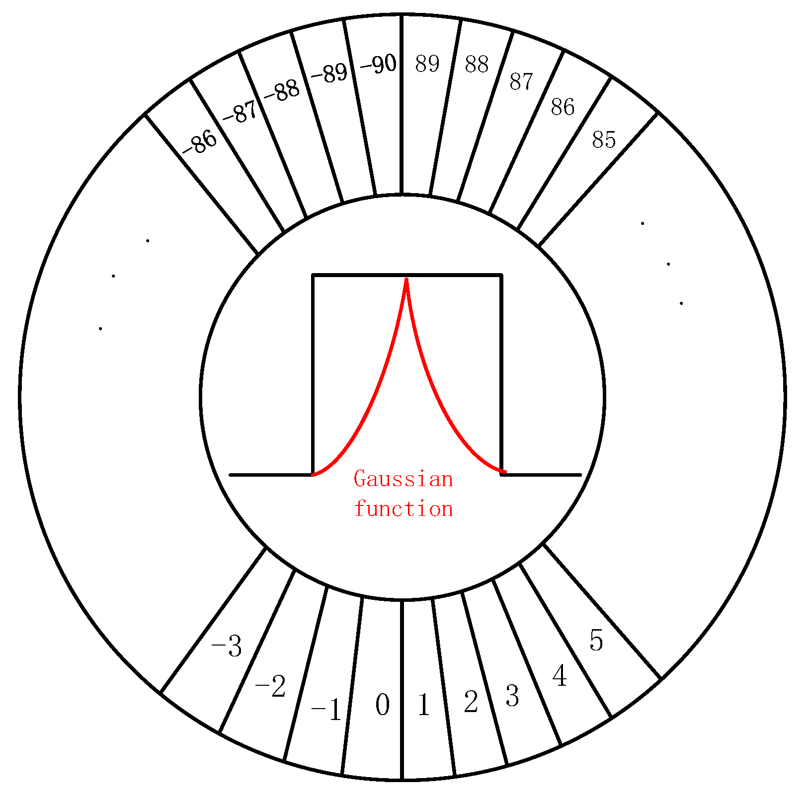
  • We used CSL to determine the angle of rotating objects, thereby turning the angle regression problem into a classification problem and more accurately detecting objects at any angle.
  • Compared with seven other recent remote sensing target detection networks, the proposed RepVGG-YOLO network demonstrated the best performance on two public datasets.
The rest of this paper is arranged as follows. Section 2 introduces the proposed model for remote sensing image target detection. Section 3 describes the experimental validation and discusses the results. Section 4 summarizes the study.

2. Materials and Methods

In this section, we first introduce the proposed network framework for target detection in remote sensing images. Next, we present a formula derivation of the Backbone network and multi-scale pyramid structure (Neck) for extracting and processing target features. Then, we discuss the prediction structure of the proposed model and, finally, we detail the loss function of the model.

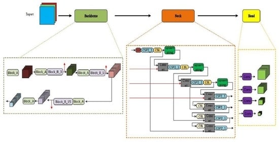
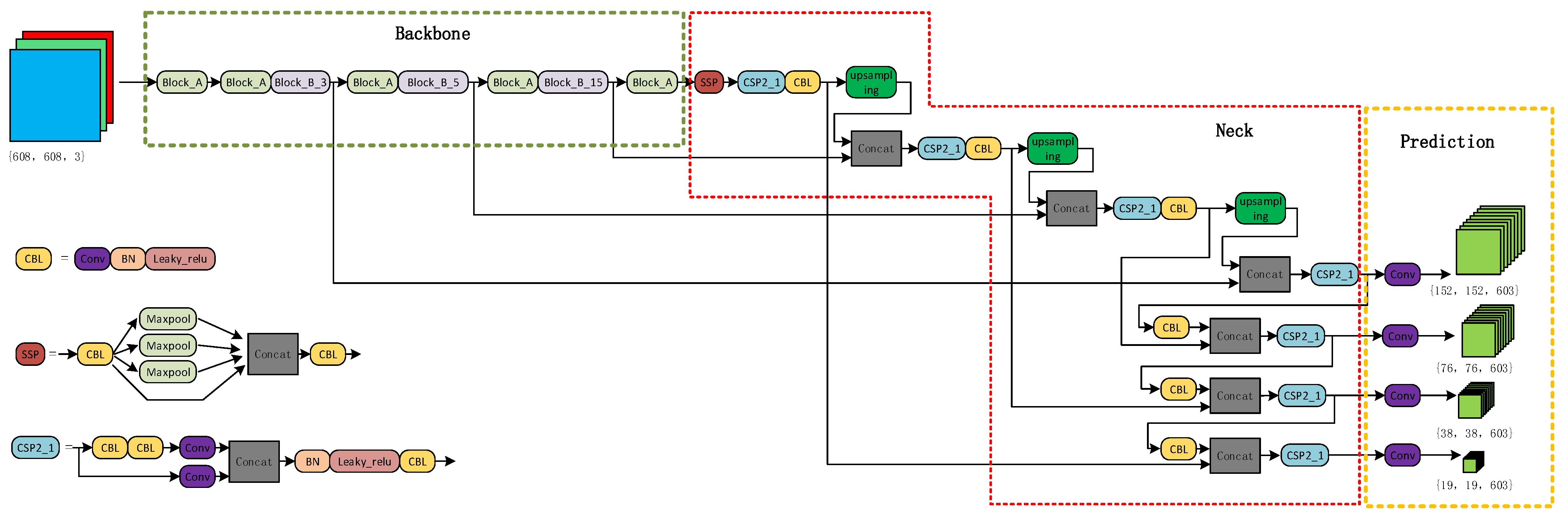
2.1. Overview of the Proposed Model

We first perform operations such as random scaling, random cropping, and random arrangement of the original dataset images, followed by data enhancement on the data to balance the size and target sample ratio and segmentation of the image with overlapping areas to retain the small target edge information. Simultaneously, we crop the original data of the different sized segments into pictures of 608 × 608 pixels, which serve as the input to the model. As shown in Figure 1, we first extract the low-level general features from the processed image through the Backbone network. To detect targets of different scales and categories, Backbone provides several combinations of receptive field size and center step length. Then, we select the corresponding feature maps from different parts of the Backbone input for Neck. Feature maps of varying sizes {152 × 152, 76 × 76, 38 × 38, 19 × 19} are selected from the hierarchical feature maps to detect targets of different sizes. By coupling the feature maps of different receptive field sizes, Neck enhances the network expressivity and distributes the multi-scale learning tasks to multiple networks. The Backbone aligns the feature maps by width once, and directly outputs the feature maps of the same width to the head network. Finally, we integrate the feature information and convert it into detection predictions. We elaborate on these parts in the following sections.

2.2. Backbone Feature Extraction Network

The Backbone network is a reference network for many computer tasks, often used to extract low-level general features, such as color, shape, and texture. It can provide several combinations of receptive field size and center step length to meet the requirements of different scales and categories in target detection. ResNet and MobileNet comprise two networks often used in various computer-vision tasks. The former can realize a combination of different resolution features and extract a robust feature representation. The latter, with its faster inference speed and fewer network parameters, finds use in embedded devices with low computing power. The RepVGG [50] model has improved speed and accuracy compared with Resnet34, ResNet50, ResNet101, ResNet152, and VGG-16. While MobileNet and VGG have improved inference speed compared with models such as VGG-16, they have lower accuracy. Therefore, considering both accuracy and inference speed, we use the improved RepVGG as the backbone network in this study. The network improvements arise from VGG network enhancements: identity and residual branches are added to the VGG network block to utilize the advantages of the ResNet network. On the basis of the RepVGG-B [50] network, we add a Block_A module at the end of the network to enhance feature extraction and, at the same time, pass the feature map input of a specific shape to the subsequent network. Figure 2 shows the execution process of the backbone feature extraction network. The two-dimensional convolution in the Block_A module has a step size of 2; thus, the feature map size will be halved after the Block_A module. Similarly, because the two-dimensional convolution in the Block_B module has a step size of 1, the size of the feature map remains unchanged after the Block_B module.
For the input picture size of 608 × 608, Figure 2 shows the shape of the output feature map of each layer. After each continuous Block_B module (Block_B_3, Block_B_5, Block_B_15), a branch is output, and the high-level features are passed to the subsequent network for feature fusion, thereby enhancing the feature extraction capability of the model. Finally, the feature map with the shape {19, 19, 512} is passed to strengthen the feature extraction network.
In addition, different network architectures are used in the training and inference stages while considering training accuracy and inference speed. Figure 3 shows the training and structural re-parameterization network architectures.
Figure 3a shows the training network of the RepVGG. The network uses two branch structures: the residual structure that contains only Block_A of the Conv1*1 residual branch, the residual structure of Conv1*1, and the identity residual; and structure Block_B. Because the training network has multiple gradient flow paths, a deeper network model can not only handle the problem of gradient disappearance in the deep layer of the network, but also obtain a more robust feature representation in the deep layer.
Figure 3b shows that RepVGG converts the multi-channel training model to a single-channel test model. To improve the inference speed, the convolutional and batch normalization (BN) layers are merged. Equations (1) and (2) express the formulas for the convolutional and BN layers, respectively.
Conv(x)=W(x)+b
BN ( x ) = γ ( x mean ) σ +   β
Replacing the argument in the BN layer equation with the convolution layer formula yields the following:
BN ( Conv ( x ) ) = γ W ( x ) σ + γ ( b mean ) σ + β = γ W ( x ) σ + γ μ σ + β
Here, μ, σ, γ, and β represent the cumulative average, standard deviation, scaling factor, and deviation, respectively. We use W k   ϵ   R C 2 × C 1 × k × k to represent the input C 1 , the output C 2 , and the convolution kernel of the convolution of k. With M 1   ϵ   R N × C 1 × H 1 × W 1 and M 2   ϵ   R N × C 2 × H 2 × W 2 denoting the input and output, respectively, the BN layer of the fusion convolution can be simplified to yield the following:
W i , : , : , : = γ i σ i   W i , : , : , : b i = μ i γ i σ i   W i , : , : , : + β i BN ( M W , μ , σ , γ , β ) : ,   i ,   : , : = ( M W   ) : , i , : , : + b i   }
where i ranges in the interval from 1 to C 2 ; * represents the convolution operation; and W and b i the weight and bias of the convolution after fusion, respectively. Let C 1 = C 2 , H 1 = H 2 , and W 1 = W 2 ; then, the output can be expressed as follows:
M 2 =   B N ( M 1 ×   W 3   ,   μ 3 , σ 3 , γ 3 , β 3 ) +   B N ( M 1 × W 1   ,   μ 1 , σ 1 , γ 1 , β 1 ) +   B N ( M 1   ,   μ 0 , σ 0 , γ 0 , β 0 )
where μ k , σ k , γ k , and β k represent the BN parameters obtained after the k × k convolution and μ 0 , σ 0 , γ 0 ,   and   β 0 represent the parameters of the identity branch. For the output of three different scales, we adopt the following strategy for fusion. We can regard the identity branch structure as a 1 × 1 convolution; for the Conv1*1 and the identity branches, the 1 × 1 convolution kernel can be filled and converted into a 3 × 3 convolution kernel; finally, we add the three 3 × 3 convolution kernels from the three output scales to obtain the final convolution kernel, and add the three deviations to obtain the final deviation. The Block_B module can be represented by Equation (5); further, because the Block_A module does not contain the identity branch structure, it can be represented by the first two items in Equation (5).

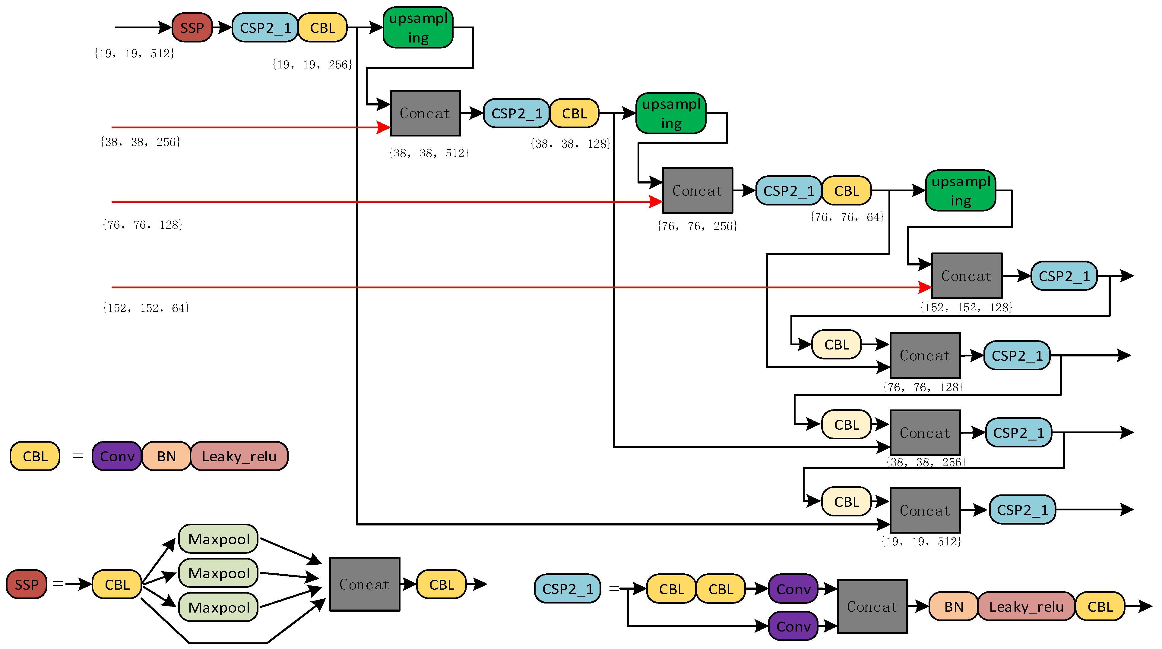
2.3. Strengthening the Feature Extraction Network (Neck)

In the target detection task, to make the model learn diverse features and improve detection performance, the Neck network can reprocess the features extracted by the Backbone, disperse the learning of different scales applied to the multiple levels of feature maps, and couple the feature maps with different receptive field sizes. In this study, we use SPP [51], improved FPN [26], and PANet [52] structure to extract the features. Figure 4 shows the detailed execution process of the model. The SPP structure uses pooling methods of different scales to perform multi-scale feature fusion, which can improve the receptive field of the model, significantly increase the receiving range of the main features, and more effectively separate the most important context features, thereby avoiding problems such as image distortion caused by cropping and zooming the image area. The computer-based learning (CBL) module comprises a two-dimensional convolution process, BN, and Leaky_ReLU activation function. The input of the CSP2_1 module is divided into two parts. One part goes through two CBL modules and then through a two-dimensional convolution; the other part directly undergoes a two-dimensional convolution operation. Finally, the feature maps obtained from the two parts are spliced, then put through the BN layer and Leaky_ReLU activation function, and output after the CBL module.
Figure 4 shows the shape of the feature map of the key parts of the entire network. Note that the light-colored CBL module (the three detection scale output parts at the bottom right) has a two-bit convolution step size of 2, whereas the other two-dimensional convolutions have a step size of 1. FPN is top-down, and transfers and integrates high-level feature information through up-sampling. FPN also transfers high-level strong semantic features to enhance the entire pyramid, but only enhances semantic information, not positioning information. We also added a bottom-up feature pyramid behind the FPN layer that accumulates low-level and processed high-level features. Because low-level features can provide more accurate location information, the additional layer creates a deeper feature pyramid, adding the ability to aggregate different detection layers from different backbone layers, which enhances the feature extraction performance of the network.

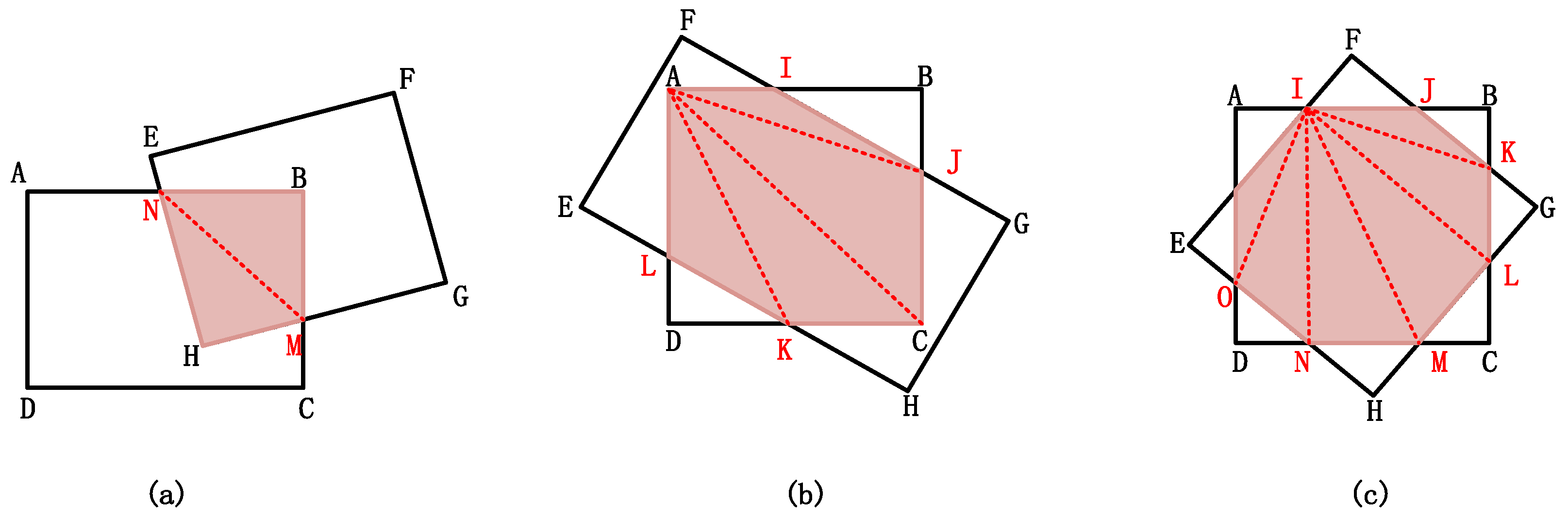
2.4. Target Boundary Processing at Any Angle

Because remote sensing images contain many complex and dense rotating targets, we need to correct these rotating objects for more accurate detection of objects at any angle. Common angle regression methods include the open source computer-vision, long edge, and ordered quadrilateral definition methods. The predictions of these methods often exceed the initial set range. Because the target parameters of learning are periodic, they can be at the boundary of periodic changes. This condition can cause a sudden increase in the loss value that increases the difficulty of learning by the network, leading to boundary problems. We use circular smooth label (CSL) [40] to handle the angle problem, as shown in Figure 5.
Equation (6) expresses CSL, where g(x) is the window function.
CSL ( x ) = { g ( x )   ,   θ r < x < θ + r 0 ,   o t h e r w i s e
where θ represents the angle passed by the longest side when the x-axis rotates clockwise, and r represents the window radius. We convert angle prediction from a regression problem to a classification problem and place the entire defined angle range into one category. We choose a Gaussian function for the window function to measure the angular distance between the predicted and ground truth labels. The predicted value loss becomes smaller the closer it comes to the true value within a certain range. Introducing periodicity, i.e., the two degrees, 89 and −90, become neighbors, solves the problem of angular periodicity. Using discrete rather than continuous angle predictions avoids boundary problems.

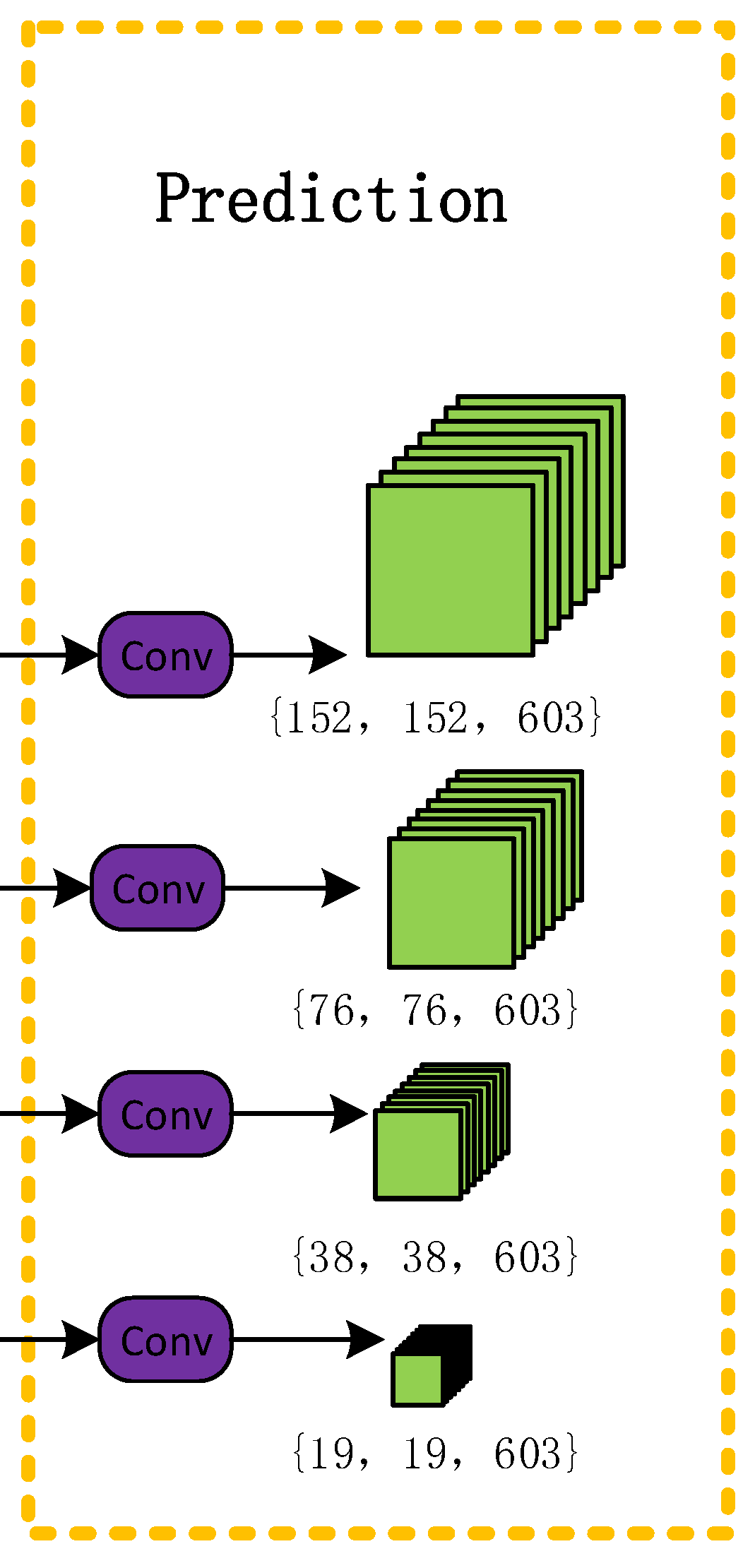
2.5. Target Prediction Network

After subjecting the image to feature extraction twice, we integrate the feature information and transform it into a prediction, as shown in Figure 6. We use the k-means clustering algorithm to generate 12 prior boxes with different scales according to the labels of the training set. Because remote sensing target detection involves detecting small targets, to enhance the feature extraction of small pixel targets, we use four detection scales with sizes of 19 × 19, 38 × 38, 76 × 76, and 152 × 152.
Taking the 19 × 19 detection scale as an example, we divide the input image into multiple 19 × 19 grids. Each grid point is preset with three boxes of corresponding scales. When these grids enclose an object, we use the corresponding grid for object detection. Finally, the shape of the feature map output by the detection feature layer is {19, 19, 603}. The third quantity implies that each of the three anchors in the corresponding grid consists of 201 dimension predictions. The width and height of the box and the coordinates of the center point (x_offset, y_offset, h, w), confidence, 16 classification results, and 180 classification angles (described in Section 2.4). Based on the set loss function (described in Section 2.6.3), iterative calculations for the backpropagation operation are performed and the position and angle of the prediction box are continually adjusted and, finally, to attain the highest confidence test results, non-maximum suppression screening is applied [53].

2.6. Loss Function

In this section, we describe the bounding box regression loss function, the confidence loss function with weight coefficients, and the classification loss function with increased angle calculation.

2.6.1. Bounding Box Border Regression Loss

The most commonly used indicator in target detection, often used to calculate the bounding box regression loss, the intersection over union (IoU) [54] value, is defined as the ratio of the intersection and union of the areas of two rectangular boxes. Equation (7) shows the IoU and the bounding box regression loss.
I o U = | B   B g t | | B   B g t | LOSS IoU = 1 I o U }
where B represents the predicted bounding box, B g t represents the real bounding box, | B   B g t | represents the B and B g t intersection area, and | B   B g t | represents the B and B g t union area. The following problems arise in calculating the loss function defined in Equation (7):
1. When B and B g t do not intersect, IoU = 0, the distance between B and B g t cannot be expressed, and the loss function LOSS_IoU cannot be directed or optimized.
2. When the size of B remains the same in different situations, the IoU values obtained do not change, making it impossible to distinguish different intersections of B and B g t .
To overcome these problems, the generalized IoU (GIoU) [55] was proposed in 2019, with the formulation shown below:
G I o U = I o U | C   ( B   B g t ) | | C | LOSS GIoU = 1 G I o U } ,
where | C | represents the area of the smallest rectangular box containing B and B g t , and | C   \ ( B   B g t ) | represents the area of the C rectangle excluding | B   B g t | . The calculation of the bounding box frame regression loss uses the GIoU. Compared with using the IoU, using the GIoU improves the measurement method of the intersection scale and alleviates the above-mentioned problems to a certain extent, but still does not consider the situation when B is inside B g t . Furthermore, when the size of B remains the same and the position changes, the GIoU value also remains the same, and the model cannot be optimized.
In response to this situation, distance-IoU (DIoU) [56] was proposed in 2020. Based on IoU and GIoU, and incorporating the center point of the bounding box, DIoU can be expressed as follows:
  D I o U = 1 I o U + ρ 2 ( B ,   B g t ) c 2 LOSS DIoU = 1 D I o U } ,
where ρ 2 ( B ,   B g t ) represents the Euclidean distance between the center points of B and B g t , and c represents the diagonal distance of the smallest rectangle that can cover B and B g t simultaneously. LOSSDIoU can be minimized by calculating the distance between B and B g t and using the distance between the center points of B and B g t as a penalty term, which improves the convergence speed.
Using both GIoU and DIoU, recalculating the aspect ratio of B and B g t , and increasing the impact factor av, the complete IoU (CIoU) [56] was proposed, as expressed below:
C I o U = I o U ρ 2 ( B ,   B g t ) c 2 a v a = v 1 I O U + v v = 4 π 2   ( a r c tan w g t h g t a r c tan w h ) 2 LOSS CIoU = 1 I o U + ρ 2 ( B ,   B g t ) c 2 + a v }
where h g t and w g t are the length and width of B g t , respectively; h and w are the length and width of B , respectively; a is the weight coefficient; and v is the distance between the aspect ratios of B and B g t . We use LOSS CIoU as the bounding box border regression loss function, which brings the predicted bounding box more in line with the real bounding box, and improves the model convergence speed, regression accuracy, and detection performance.

2.6.2. Confidence Loss Function

We use cross-entropy to calculate the object confidence loss. Regardless of whether there is an object to be detected in the grid, the confidence error must be calculated. Because only a small part of the input image may contain objects to be detected, we add a weight coefficient ( λ n o ) to constrain the confidence loss for the image area that does not contain the target object, thereby reducing the number of negative samples. The object confidence loss can be expressed as follows:
LOSS Conf =   i = 0 S 2 j = 0 B I i j ( C ^ i j log C i j + ( 1 C ^ i j ) log ( 1 C i j ) ) R I o u   + ( 1 I i j ) ( C ^ i log C i + ( 1 C ^ i j ) log ( 1 C i ) ) λ n o .
where S is the number of grids in the network output layer and B is the number of anchors. I i j indicates whether the j-th anchor in the i-th grid can detect this object (the detected value is 1 and the undetected value is 0), and the value of C ^ i j is determined by whether the bounding box of the grid is responsible for predicting an object (if it is responsible for prediction, the value of C ^ i j is 1, otherwise it is 0). C i j is the predicted value after parameter normalization (the value lies between 0 and 1). R I o u represents the IoU of the rotating bounding box.
The complete decoupling of the correlation between the prediction angle and the prediction confidence means the confidence loss is not only related to the frame parameters, but also to the rotation angle. Table 1 summarizes the recalculation of the IoU [35] of the rotating bounding box as the confidence loss coefficient, along with its pseudocode.
Figure 7 shows the geometric principle of rotating IoU calculations. We divide the overlapping part into multiple triangles with the same vertex, calculate the area of each triangle separately, and finally add the calculated areas to obtain the area of the overlapping polygons. The detailed calculation principle is as follows. Given a set of rotating rectangles R1, R2, …, RN, calculate the RIoU of each pair of <Ri, Rj>. First, the intersection set, PSet, of Ri and Rj (the intersection of two rectangles and the vertices of one rectangle in the other rectangle form a set, PSet, corresponding to rows 4–7 of Table 1); then, calculate the intersection area, I, of PSet and, finally, calculate the RIoU according to the formula in row 10 of Table 1 (combine the points generated by the PSet into a polygon, divide the polygon into multiple triangles, calculate the sum of the area of the multiple triangles as the polygon area, and finally calculate the polygon area and remove the rotation of the polygon area; corresponding to rows 8–10 of Table 1).

2.6.3. Classification Loss Function

Because we converted the angle calculation from a regression problem into a classification problem, we calculate both the category and angle loss when calculating the classification loss function. Here, we use the cross-entropy loss function for the calculation. When the j-th anchor box of the i-th grid is responsible for a real target, we calculate the classification loss function for the bounding box generated by this anchor box, using Equation (12).
LOSS Class = i = 0 S 2 j = 0 B I i j c C l a s s ,   θ ( 0 , 180 ] ( P i ^ ( c + θ ) log P i ( c + θ ) + ( 1 P i ^ ( c + θ ) ) log ( 1 P i ( c + θ ) ) )
where c belongs to the target classification category; θ belongs to the angle processed by the CSL [40] algorithm; S is the number of grids in the network output layer; B is the number of anchors; and I i j indicates whether the j-th anchor in the i-th grid can detect this object (the detected value is 1 and the undetected value is 0).
The final total loss function equals the sum of the three loss functions, as shown in Equation (13). Furthermore, the three loss functions have the same effect on the total loss function; that is, the reduction of any one of the loss functions will lead to the optimization of the total loss function.
L O S S = LOSS CIoU + LOSS Conf + LOSS Class

3. Experiments, Results, and Discussion

3.1. Introduction to DOTA and HRSC2016 Datasets

3.1.1. DOTA Dataset

The DOTA dataset [57] comprises 2806 aerial images obtained from different sensors and platforms, including 15 classification categories: plane (PL), baseball diamond (BD), bridge (BR), ground track (GTF), small vehicle (SV), large vehicle (LV), ship (SH), tennis court (TC), basketball court (BC), oil storage tank (ST), football field (SBF), roundabout (RA), airport and helipad (HA), swimming pool (SP), and helicopter (HC). The image data can be divided into 1411 training sets, 937 test sets, and 458 verification sets. The image size ranges between 800 × 800 and 4000 × 4000 pixels. Dataset labeling consisted of a horizontal and a directional bounding box for a total of 188,282 instances.

3.1.2. HRSC2016 Dataset

The HRSC2016 dataset [58] comes from six different ports, with a total of 1061 remote sensing pictures. Examples of detection objects include ships on the sea and ships docked on the shore. The images can be divided into 436 training sets (1207 labeled examples in total), 444 test sets (1228 labeled examples in total), and 181 validation sets (541 labeled examples in total). The image size ranges from 300 × 300 to 1500 × 900 pixels.

3.2. Image Preprocessing and Parameter Optimization

In this section, we describe image preprocessing, experimental parameter settings, and experimental evaluation standards.

3.2.1. Image Preprocessing

Owing to the complex background of remote sensing target detection [59], large changes in the target scale [60], special viewing angle [61,62,63], unbalanced categories [31], and so on, we preprocess the original data. Directly processing the original high-resolution remote sensing images not only increases equipment requirements, but also significantly reduces detection accuracy. We cut the entire picture and send it to the proposed model training module. During the test, we cut the test pictures into pictures of the same size as those in the training set, and after the test, we splice the predicted results one by one to obtain the total result. To ensure the loss of small target information at the cutting edge during the cutting process, we allow the cut image to have a certain proportion of overlap area (in this study, we set the overlap area to 30%). If the size of the original image is smaller than the size of the cut image, we perform an edge pixel filling operation on the original image to make its size reach the training size. In the remote sensing dataset (e.g., DOTA), the sample target size changes drastically, and small targets can be densely distributed and large and small targets can be considerably unevenly distributed (the number of small targets is much larger than the number of large targets). In this regard, we use the Mosaic data enhancement method to splice the pictures in random zooming, cropping, and arrangement, which substantially enriches the dataset and makes the distribution of targets of different sizes more uniform. Mixed multiple images can have different semantics. Enhanced network robustness occurs when the picture information allows the detector to detect targets beyond the conventional context.

3.2.2. Experimental Parameter Settings

We evaluated the performance of the proposed model on two NVIDIA GeForce RTX 2080 Ti GPUs with 11 GB of RAM. We used the PyTorch 1.7 deep learning framework and Python 3.7 compiler run on Windows 10. To optimize the network, we used stochastic gradient descent with momentum, setting the learning rate momentum and weight decay coefficients to 0.857 and 0.00005, respectively; the iterative learning rate for the first 50 K to 0.001; and the later iterative learning rate to 0.0001. The CIoU loss and classification loss coefficients were set to 0.0337 and 0.313, respectively. The weight coefficient, λ n o , of the confidence loss function was set to 0.4. The batch size was set to eight, and the epoch was set to 500.

3.2.3. Evaluation Criteria

To verify the performance of the proposed method, two broad criteria were used to evaluate the test results [64]: precision and recall. The accuracy rate indicates the detection rate of the predicted true-positive samples, and the recall rate indicates the rate of correctly identified true-positive samples. Accuracy and recall can be expressed as follows.
Precision = TP T P + F P
Recall = TP T P + F N
TP represents a real positive sample, TN represents a real negative sample, FP is a false positive sample, and FN is a false negative sample. This study adopts the mean average precision (mAP) [45,46,47] to evaluate all methods, which can be expressed as follows:
mAP = i = 1 N c l a s s   P i ( R i ) d R i N c l a s s
where P i and R i represent the accuracy and recall rate of the i-th class of classified objects, respectively. N c l a s s represents the total number of detected objects in the dataset.

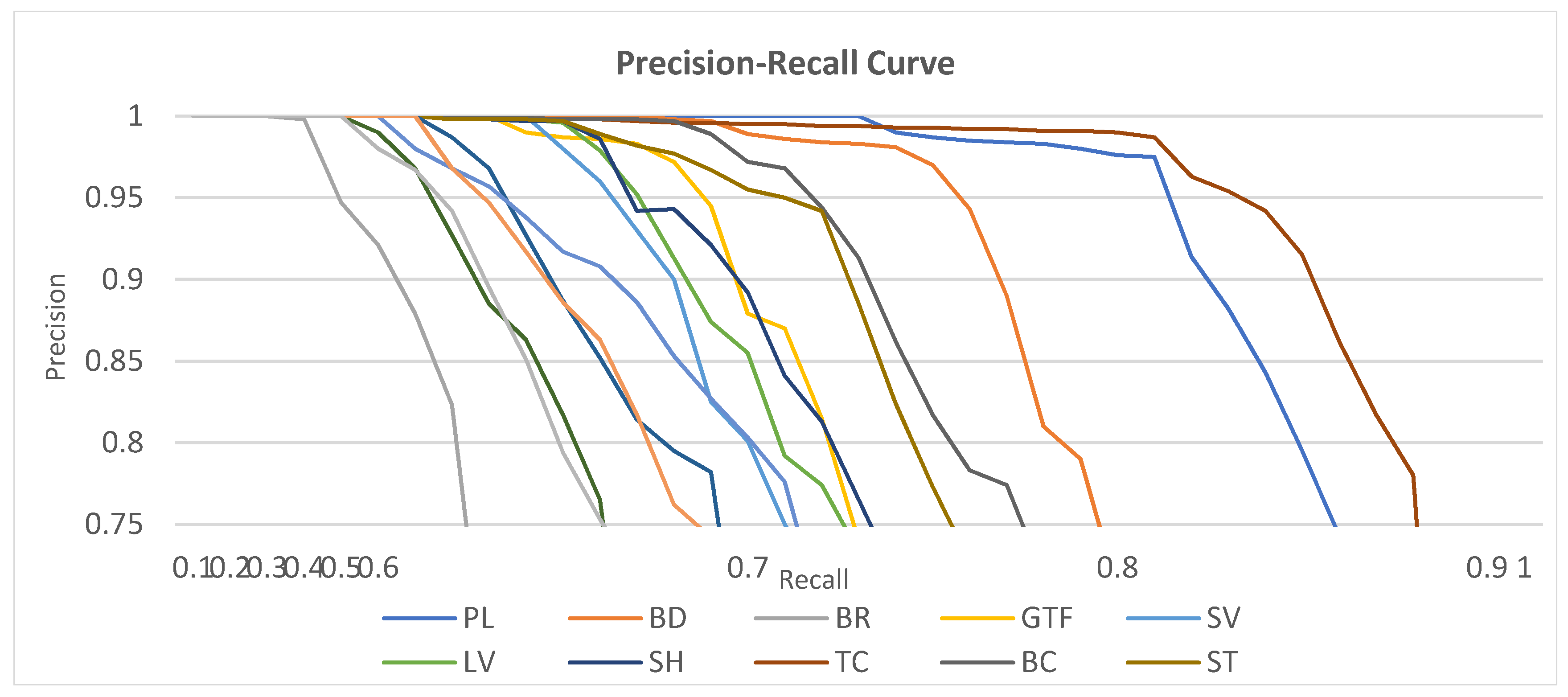
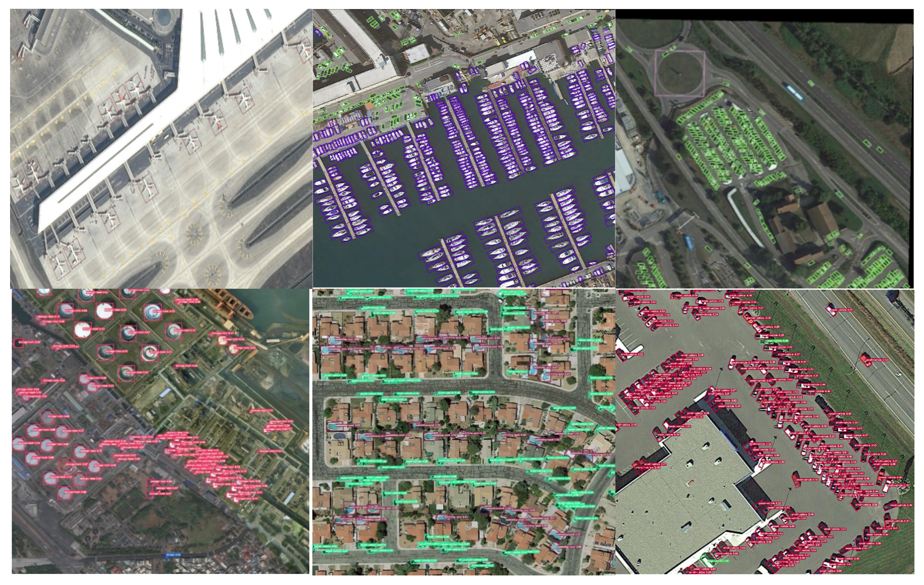
3.3. Experimental Results

Figure 8 shows the precision–recall curve of the DOTA detection object category. We focus on the interval between 0.6 and 0.9, where the recall rate is concentrated. Except for BR, when the recall value is greater than 0.6, the decline in the curves of the other types of objects increases. The BD, PL, and TC curves all drop sharply when the recall value is greater than 0.8. The results show that the overall performance of the proposed method is stable and has good detection effectiveness.
To prove that the proposed method has better performance, we compared the proposed method (RepVGG-YOLO NET) to seven other recent methods: SSD [20], joint training method for target detection and classification (YOLOV2) [19], rotation dense feature pyramid network (R-DFPN) [39], toward real-time object detection with RPN (FR-C) [25], joint image cascade and functional pyramid network and multi-size convolution kernel to extract multi-scale strong and weak semantic feature framework (ICN) [36], fine FPN and multi-layer attention network (RADET) [65], and end-to-end refined single-stage rotation detector (R3Det) [66]. Table 2 summarizes the quantitative comparison results of the eight methods on the DOTA dataset. The table indicates that the proposed model has achieved the most advanced results, achieving relatively stable detection results in all categories, with an mAP of 74.13%. SSD and YOLOV2 networks have poor detection effectiveness and relatively low detection effectiveness on small targets; their poor feature extraction network performance needs improvement. The FR-C, ICN, and RADET network models achieved good detection results.
Compared with other methods, owing to the increased processing of targets at any angle and the use of four target detection scales, the proposed model achieved good classification results for small objects with complex backgrounds and dense distributions (for example, SV and SH achieved 71.02% and 78.41% mAP values). Compared with the suboptimal method (i.e., R3Det), the suggested method achieved a 1.32% better mAP value. In addition, using the FPN and PANet structures to accumulate high-level and low-level features helped the improvement in the detection of categories with large differences in the target scale of the same image (for example, BR and LV on the same image), with BR and LV achieving classification results of 52.34% and 76.27%, respectively. We also obtained relatively stable mAP values in single-category detection (PL, BR, SV, LV, TC, BC, SBF, RA, SP, and HC achieved the highest mAP values).
Table 3 summarizes the proposed model and five other methods (i.e., rotation-sensitive regression for oriented scene text detection (RRD) [67], rotated region-based CNN for ship detection (BL2 and RC2) [68], refined single-stage detector with feature refinement for rotating object (R3 DET) [66], and rotated region proposal and discrimination networks (R2PN) [69]). Table 3 summarizes quantitative comparison results on the HRSC2016 dataset. The results demonstrate that the proposed method achieves an mAP detection result of 91.54, which is better than the other methods evaluated on this dataset. Compared with the suboptimal method (R3Det), the mAP for the proposed model was better by 2.21%. Good results were achieved for the detection of ship instances with large aspect ratios and rotation directions. The proposed method achieved 22 frames per second (FPS), which is more than that achieved by the suboptimal method (R3Det).
Figure 9 shows the partial visualization results of the proposed method on the DOTA and HRSC2016 datasets. The first three rows are the visualization results of the DOTA dataset, and the last row shows the visualization results of the HRSC2016 dataset. Figure 9 shows that the proposed model handles well the noise problem in a complex environment, and has a better detection effectiveness on densely distributed small objects. Good test results were also obtained for some samples with drastic size changes and special viewing angles.

3.4. Ablation Study

We conducted a series of comparative experiments on the DOTA data set, as shown in Table 4. We considered the influence of different combinations of the five factors of backbone network, bounding box border regression loss (BBRL), data enhancement (DE), multi-scale settings, and CSL on the final experimental results. We used mAP and FPS as evaluation criteria to verify the effectiveness of our method.
From Table 4, the first row is the baseline, the improved RepVGG-A is used as the backbone, and the DIou is used as the BBRL. The backbone network is a reference network for many computer tasks. We set the first and third groups, and the second combination and the fourth group of experiments to verify the backbone network. The results show that RepVGG-B has more complex network parameters and is deeper than RepVGG-A. Consequently, using the improved RepVGG-B as the backbone (groups 3 and 4), mAP increased by 1.05% and 2.79%, respectively. Choosing an appropriate loss function can improve the convergence speed and prediction accuracy of the model. Here, we set the first group, the second group, and the third combination and the fourth group of experiments to analyze the BBRL. Because CIou recalculated the predicted bounding box, the aspect ratio of the bounding box and the real bounding box increased, and the influence factor increased to align the predicted bounding box with the actual box. Under the same conditions, better results were obtained when CIou was used as the BBRL. The objective of DE is to increase the number and diversity of samples, which can significantly improve the problem of sample imbalance. According to the experimental results of the fourth and fifth groups, mAP increased by 1.06% after the image was processed by cropping, zooming, and random arrangement. Because different detection scales have different sensitivities to objects of different scales, there are many detection targets with large differences in size in remote sensing images. We can observe from the experimental results of the fifth and sixth groups that mAP improved by 1.21% when four detection scales were used. The increased number of detection scales enhances the detection of small target objects. Because there are many dense rotating targets in remote sensing images, we assume that the bounding box can be predicted more accurately. Next, we set up the sixth and seventh groups of experiments. The results show that, after using CSL, we can change the angle prediction from a regression problem into a classification problem, and the periodicity problem of the angle was solved. mAP improved by 1.88% to 74.13%. We finally chose the improved RepVGG-B model as the backbone network with CIou as the BBRL loss function, using DE, Multi scale, and CSL simultaneously, and finally obtaining RepVGG-YOLO NET.

4. Conclusions

In this article, we introduce a method for detecting targets from arbitrary-angle geographic remote sensing. A RepVGG-YOLO model is proposed, which uses an improved RepVGG module as the backbone feature extraction network (Backbone) of the model, and uses SPP, feature pyramid network (FPN), and path aggregation network (PANet) as the enhanced feature extraction networks. The model combines context information on multiple scales, accumulates multi-layer features, and strengthens feature information extraction. In addition, we use four target detection scales to enhance the feature extraction of remote sensing small target pixels and the CSL method to increase the detection accuracy of objects at any angle. We redefine the classification loss function and add the angle problem to the loss calculation. The proposed model achieved the best detection performance among the eight methods evaluated. The proposed model obtained an mAP of 74.13% and 22 FPS on the DOTA dataset, wherein the mAP value exceeded that of the suboptimal method (R3Det) by 1.32%. The proposed model obtained an mAP of 91.54% on the HRSC2016 dataset. The mAP value and the FPS exceeded that of the suboptimal method (R3Det) by 2.21% and 13, respectively. We expect to conduct further research on the detection of blurred, dense small objects and obscured objects.

Author Contributions

Conceptualization, Y.Q. and W.L.; methodology, Y.Q.; software, Y.Q. and W.L.; validation, Y.Q., L.F. and W.G.; formal analysis, Y.Q. and L.F.; writing—original draft preparation, Y.Q., W.L. and L.F.; writing—review and editing, Y.Q. and W.L.; visualization, Y.Q. and W.L. All authors have read and agreed to the published version of the manuscript.

Funding

This research received no external funding.

Data Availability Statement

Not applicable.

Acknowledgments

The authors would like to thank Guigan Qing and Chaoxiu Li for their support, secondly, thanks to Lianshu Qing and Niuniu Feng for their support.

Conflicts of Interest

The authors declare no conflict of interest.

References

  1. Zhang, F.; Du, B.; Zhang, L.; Xu, M. Weakly supervised learning based on coupled convolutional neural networks for aircraft detection. IEEE Trans. Geosci. Remote Sens. 2016, 54, 5553–5563. [Google Scholar] [CrossRef]
  2. Kamusoko, C. Importance of remote sensing and land change modeling for urbanization studies. In Urban Development in Asia and Africa; Springer: Singapore, 2017. [Google Scholar]
  3. Ahmad, K.; Pogorelov, K.; Riegler, M.; Conci, N.; Halvorsen, P. Social media and satellites. Multimed. Tools Appl. 2019, 78, 2837–2875. [Google Scholar] [CrossRef]
  4. Tang, T.; Zhou, S.; Deng, Z.; Zou, H.; Lei, L. Vehicle detection in aerial images based on region convolutional neural networks and hard negative example mining. Sensors 2017, 17, 336. [Google Scholar] [CrossRef] [Green Version]
  5. Cheng, G.; Zhou, P.; Han, J. RIFD-CNN: Rotation-invariant and fisher discriminative convolutional neural networks for object detection. In Proceedings of the IEEE Conference on Computer Vision and Pattern Recognition (CVPR), Las Vegas, NV, USA, 26 June–1 July 2016; pp. 2884–2893. [Google Scholar]
  6. Deng, Z.; Sun, H.; Zhou, S.; Zhao, J.; Zou, H. Toward fast and accurate vehicle detection in aerial images using coupled region-based convolutional neural networks. J-STARS 2017, 10, 3652–3664. [Google Scholar] [CrossRef]
  7. Long, Y.; Gong, Y.; Xiao, Z.; Liu, Q. Accurate object localization in remote sensing images based on convolutional neural networks. IEEE Trans. Geosci. Remote Sens. 2017, 55, 2486–2498. [Google Scholar] [CrossRef]
  8. Crisp, D.J. A ship detection system for RADARSAT-2 dual-pol multi-look imagery implemented in the ADSS. In Proceedings of the 2013 IEEE International Conference on Radar, Adelaide, Australia, 9–12 September 2013; pp. 318–323. [Google Scholar]
  9. Wang, C.; Bi, F.; Zhang, W.; Chen, L. An intensity-space domain CFAR method for ship detection in HR SAR images. IEEE Geosci. Remote Sens. Lett. 2017, 14, 529–533. [Google Scholar] [CrossRef]
  10. Leng, X.; Ji, K.; Zhou, S.; Zou, H. An adaptive ship detection scheme for spaceborne SAR imagery. Sensors 2016, 16, 1345. [Google Scholar] [CrossRef] [PubMed] [Green Version]
  11. Krizhevsky, A.; Sutskever, I.; Hinton, G.E. Imagenet classification with deep convolutional neural networks. NIPS 2012, 25, 1097–1105. [Google Scholar] [CrossRef]
  12. Xie, S.; Girshick, R.; Dollár, P.; Tu, Z.; He, K. Aggregated residual transformations for deep neural networks. In Proceedings of the IEEE Conference on Computer Vision and Pattern Recognition (CVPR), Honolulu, HI, USA, 21–26 July 2017; pp. 1492–1500. [Google Scholar]
  13. Chen, K.; Pang, J.; Wang, J.; Xiong, Y.; Li, X.; Sun, S.; Feng, W.; Liu, Z.; Shi, J.; Ouyang, W.; et al. Hybrid task cascade for instance segmentation. arXiv 2019, arXiv:1901.07518. [Google Scholar]
  14. Li, B.; Yan, J.; Wu, W.; Zhu, Z.; Hu, X. High performance visual tracking with Siamese region proposal network. In Proceedings of the IEEE Conference on Computer Vision and Pattern Recognition (CVPR), Salt Lake City, UT, USA, 18–22 June 2018; pp. 8971–8980. [Google Scholar]
  15. Tian, L.; Cao, Y.; He, B.; Zhang, Y.; He, C.; Li, D. Image Enhancement Driven by Object Characteristics and Dense Feature Reuse Network for Ship Target Detection in Remote Sensing Imagery. Remote Sens. 2021, 13, 1327. [Google Scholar] [CrossRef]
  16. Li, Y.; Li, X.; Zhang, C.; Lou, Z.; Zhu, Y.; Ding, Z.; Qin, T. Infrared Maritime Dim Small Target Detection Based on Spatiotemporal Cues and Directional Morphological Filtering. Infrared Phys. Technol. 2021, 115, 103657. [Google Scholar] [CrossRef]
  17. Yao, Z.; Wang, L. ERBANet: Enhancing Region and Boundary Awareness for Salient Object Detection. Neurocomputing 2021, 448, 152–167. [Google Scholar] [CrossRef]
  18. Redmon, J.; Divvala, S.; Girshick, R.; Farhadi, A. You only look once: Unified, real-time object detection. In Proceedings of the IEEE Conference on Computer Vision and Pattern Recognition (CVPR), Las Vegas, NV, USA, 26 June–1 July 2016; pp. 779–788. [Google Scholar]
  19. Redmon, J.; Farhadi, A. YOLO9000: Better, faster, stronger. In Proceedings of the IEEE Conference on Computer Vision and Pattern Recognition (CVPR), Honolulu, HI, USA, 21–26 July 2017; pp. 7263–7271. [Google Scholar]
  20. Liu, W.; Anguelov, D.; Erhan, D.; Szegedy, S.; Reed, S.; Fu, C.-Y.; Berg, A.C. SSD: Single shot multibox detector. In Proceedings of the European Conference on Computer Vision, Amsterdam, The Netherlands, 11–14 October 2016; Springer: Cham, Switzerland, 2016; pp. 21–37. [Google Scholar]
  21. Lin, T.-Y.; Goyal, P.; Girshick, R.; He, K.; Dollár, P. Focal loss for dense object detection. In Proceedings of the IEEE International Conference on Computer Vision (ICCV), Venice, Italy, 22–29 October 2017; pp. 2980–2988. [Google Scholar]
  22. Girshick, R.; Donahue, J.; Darrell, T.; Malik, J. Region-based convolutional networks for accurate object detection and segmentation. IEEE Trans. Pattern Anal. Mach. Intell. 2016, 38, 142–158. [Google Scholar] [CrossRef]
  23. Girshick, R. Fast R-CNN. In Proceedings of the IEEE International Conference on Computer Vision (ICCV), Araucano Park, Las Condes, Chile, 11–18 December 2015; pp. 1440–1448. [Google Scholar]
  24. Ren, S.; He, K.; Girshick, R.; Sun, J. Faster R-CNN: Towards real-time object detection with region proposal networks. IEEE Trans. Pattern Anal. Mach. Intell. 2017, 39, 1137–1149. [Google Scholar] [CrossRef] [PubMed] [Green Version]
  25. Dai, J.; Li, Y.; He, K.; Sun, J. R-FCN: Object detection via region-based fully convolutional networks. NIPS 2016, 29, 379–387. [Google Scholar]
  26. Lin, T.-Y.; Dollár, P.; Girshick, R.; He, K.; Hariharan, B.; Belongie, S. Feature pyramid networks for object detection. In Proceedings of the IEEE Conference on Computer Vision and Pattern Recognition (CVPR), Honolulu, HI, USA, 21–26 July 2017; pp. 2117–2125. [Google Scholar]
  27. Li, Y.; Zhang, Y.; Huang, X.; Yuille, A.L. Deep networks under scene-level supervision for multi-class geospatial object detection from remote sensing images. ISPRS J. Photogramm. Remote Sens. 2018, 146, 182–196. [Google Scholar] [CrossRef]
  28. Ming, Q.; Miao, L.; Zhou, Z.; Dong, Y. CFC-Net: A critical feature capturing network for arbitrary-oriented object detection in remote sensing images. arXiv 2021, arXiv:2101.06849. [Google Scholar]
  29. Pang, J.; Li, C.; Shi, J.; Xu, Z.; Feng, H. R2-CNN: Fast tiny object detection in large-scale remote sensing images. IEEE Trans. Geosci. Remote Sens. 2019, 57, 5512–5524. [Google Scholar] [CrossRef] [Green Version]
  30. Han, J.; Ding, J.; Li, J.; Xia, G.S. Align deep features for oriented object detection. IEEE Trans. Geosci. Remote Sens. 2021, 1–11. [Google Scholar]
  31. Deng, Z.; Sun, H.; Zhou, S.; Zhao, J.; Lei, L.; Zou, H. Multi-scale object detection in remote sensing imagery with convolutional neural networks. ISPRS J. Photogramm. Remote Sens. 2018, 145, 3–22. [Google Scholar] [CrossRef]
  32. Feng, P.; Lin, Y.; Guan, J.; He, G.; Shi, H.; Chambers, J. TOSO: Student’s-T distribution aided one-stage orientation target detection in remote sensing images. In Proceedings of the 2020 IEEE International Conference on Acoustics, Speech and Signal Processing (ICASSP), Barcelona, Spain, 4–8 May 2020; pp. 4057–4061. [Google Scholar]
  33. Xu, Y.; Fu, M.; Wang, Q.; Wang, Y.; Chen, K.; Xia, G.; Bai, X. Gliding vertex on the horizontal bounding box for multi-oriented object detection. IEEE Trans. Pattern Anal. Mach. Intell. 2021, 43, 1452–1459. [Google Scholar] [CrossRef] [Green Version]
  34. Ding, J.; Xue, N.; Long, Y.; Xia, G.S.; Lu, Q. Learning RoI Transformer for Detecting Oriented Objects in Aerial Images. In Proceedings of the IEEE/CVF Conference on Computer Vision and Pattern Recognition, Los Angeles, CA, USA, 16–19 June 2019. [Google Scholar]
  35. Xia, G.S.; Bai, X.; Ding, J.; Zhu, Z.; Belongie, S.; Luo, J.; Datcu, M.; Pelillo, M.; Zhang, L. DOTA: A Large-Scale Dataset for Object Detection in Aerial Images. In Proceedings of the IEEE Conference on Computer Vision and Pattern Recognition, Salt Lake City, UT, USA, 18–23 June 2018; pp. 3974–3983. [Google Scholar]
  36. Azimi, S.M.; Vig, E.; Bahmanyar, R.; Körner, M.; Reinartz, P. Towards multi-class object detection in unconstrained remote sensing imagery. arXiv 2018, arXiv:1807.02700. [Google Scholar]
  37. Liu, L.; Pan, Z.; Lei, B. Learning a rotation invariant detector with rotatable bounding box. arXiv 2017, arXiv:1711.09405. [Google Scholar]
  38. Wang, J.; Ding, J.; Guo, H.; Cheng, W.; Pan, T.; Yang, W. Mask OBB: A Semantic Attention-Based Mask Oriented Bounding Box Representation for Multi-Category Object Detection in Aerial Images. Remote Sens. 2019, 11, 2930. [Google Scholar] [CrossRef] [Green Version]
  39. Yang, X.; Sun, H.; Fu, K.; Yang, J.; Sun, X.; Yan, M.; Guo, Z. Automatic ship detection in remote sensing images from Google Earth of complex scenes based on multiscale rotation dense feature pyramid networks. Remote Sens. 2018, 10, 132. [Google Scholar] [CrossRef] [Green Version]
  40. Yang, X.; Yan, J. Arbitrary-oriented object detection with circular smooth label. In Proceedings of the 16th European Conference on Computer Vision, Glasgow, UK, 23–28 August 2020; Springer: Cham, Switzerland, 2020; pp. 677–694. [Google Scholar]
  41. Chen, J.; Wan, L.; Zhu, J.; Xu, G.; Deng, M. Multi-scale spatial and channel-wise attention for improving object detection in remote sensing imagery. IEEE Geosci. Remote Sens. Lett. 2020, 17, 681–685. [Google Scholar] [CrossRef]
  42. Cui, Z.; Li, Q.; Cao, Z.; Liu, N. Dense attention pyramid networks for multi-scale ship detection in SAR images. IEEE Trans. Geosci. Remote Sens. 2019, 57, 8983–8997. [Google Scholar] [CrossRef]
  43. Zhang, G.; Lu, S.; Zhang, W. CAD-net: A context-aware detection network for objects in remote sensing imagery. IEEE Trans. Geosci. Remote Sens. 2019, 57, 10015–10024. [Google Scholar] [CrossRef] [Green Version]
  44. Zhu, Y.; Urtasun, R.; Salakhutdinov, R.; Fidler, S. segDeepM: Exploiting segmentation and context in deep neural networks for object detection. In Proceedings of the IEEE Conference on Computer Vision and Pattern Recognition (CVPR), Boston, MA, USA, 7–12 June 2015; pp. 4703–4711. [Google Scholar]
  45. Gidaris, S.; Komodakis, N. Object detection via a multi-region and semantic segmentation-aware CNN model. In Proceedings of the IEEE International Conference on Computer Vision (ICCV), Araucano Park, Las Condes, Chile, 11–18 December 2015; pp. 1134–1142. [Google Scholar]
  46. Zhang, L.; Shi, Z.; Wu, J. A hierarchical oil tank detector with deep surrounding features for high-resolution optical satellite imagery. IEEE J. Sel. Top. Appl. Earth Observ. Remote Sens. 2015, 8, 4895–4909. [Google Scholar] [CrossRef]
  47. Bell, S.; Zitnick, C.L.; Bala, K.; Girshick, R. Inside-outside net: Detecting objects in context with skip pooling and recurrent neural networks. In Proceedings of the IEEE Conference on Computer Vision and Pattern Recognition (CVPR), Las Vegas, NV, USA, 26 June–1 July 2016; pp. 2874–2883. [Google Scholar]
  48. Marcu, A.; Leordeanu, M. Dual local-global contextual pathways for recognition in aerial imagery. arXiv 2016, arXiv:1605.05462. [Google Scholar]
  49. Kang, M.; Ji, K.; Leng, X.; Lin, Z. Contextual region-based convolutional neural network with multilayer fusion for SAR ship detection. Remote Sens. 2017, 9, 860. [Google Scholar] [CrossRef] [Green Version]
  50. Ding, X.; Zhang, X.; Ma, N.; Han, J.; Ding, G.; Sun, J. RepVGG: Making VGG-style ConvNets Great Again. arXiv 2021, arXiv:2101.03697v3. [Google Scholar]
  51. He, K.; Zhang, X.; Ren, S.; Sun, J. Spatial pyramid pooling in deep convolutional networks for visual recognition. IEEE Trans. Pattern Anal. Mach. Intell. 2015, 37, 1904–1916. [Google Scholar] [CrossRef] [PubMed] [Green Version]
  52. Liu, S.; Qi, L.; Qin, H.; Shi, J.; Jia, J. Path aggregation network for instance segmentation. In Proceedings of the IEEE Conference on Computer Vision and Pattern Recognition (CVPR), Salt Lake City, UT, USA, 18–22 June 2018; pp. 8759–8768. [Google Scholar]
  53. Bai, J.; Zhu, J.; Zhao, R.; Gu, F.; Wang, J. Area-based non-maximum suppression algorithm for multi-object fault detection. Front. Optoelectron. 2020, 13, 425–432. [Google Scholar] [CrossRef]
  54. Rezatofighi, H.; Tsoi, N.; Gwak, J.Y.; Sadeghian, A.; Reid, I.; Savarese, S. Generalized intersection over union: A metric and a loss for bounding box regression. In Proceedings of the 2019 IEEE/CVF Conference on Computer Vision and Pattern Recognition (CVPR), Long Beach, CA, USA, 15–20 June 2019; pp. 658–666. [Google Scholar] [CrossRef] [Green Version]
  55. Zheng, Z.; Wang, P.; Liu, W.; Li, J.; Ye, R.; Ren, D. Distance-IoU loss: Faster and better learning for bounding box regression. In Proceedings of the AAAI Conference on Artificial Intelligence, New York, NY, USA, 7–12 February 2020; Volume 34, pp. 12993–13000. [Google Scholar] [CrossRef]
  56. Ma, J.; Shao, W.; Ye, H.; Wang, L.; Wang, H.; Zheng, Y.; Xue, X. Arbitrary-oriented scene text detection via rotation proposals. IEEE Trans. Multimed. 2018, 20, 3111–3122. [Google Scholar] [CrossRef] [Green Version]
  57. Liu, Z.; Yuan, L.; Weng, L.; Yang, Y. A high resolution optical satellite image dataset for ship recognition and some new baselines. In Proceedings of the 6th International Conference on Pattern Recognition Applications and Methods (ICPRAM), Porto, Portugal, 24–26 February 2017; pp. 324–331. [Google Scholar]
  58. Wang, C.; Bai, X.; Wang, S.; Zhou, J.; Ren, P. Multiscale visual attention networks for object detection in VHR remote sensing images. IEEE Geosci. Remote Sens. Lett. 2018, 16, 310–314. [Google Scholar] [CrossRef]
  59. Zhang, Y.; Yuan, Y.; Feng, Y.; Liu, X. Hierarchical and robust convolutional neural network for very high-resolution remote sensing object detection. IEEE Trans. Geosci. Remote Sens. 2019, 57, 5535–5548. [Google Scholar] [CrossRef]
  60. Cheng, G.; Zhou, P.; Han, J. Learning rotation-invariant convolutional neural networks for object detection in VHR optical remote sensing images. IEEE Trans. Geosci. Remote Sens. 2016, 54, 7405–7415. [Google Scholar] [CrossRef]
  61. Li, K.; Cheng, G.; Bu, S.; You, X. Rotation-insensitive and context-augmented object detection in remote sensing images. IEEE Trans. Geosci. Remote Sens. 2017, 56, 2337–2348. [Google Scholar] [CrossRef]
  62. Wu, X.; Hong, D.; Tian, J.; Chanussot, J.; Li, W.; Tao, R. ORSIm detector: A novel object detection framework in optical remote sensing imagery using spatial-frequency channel features. IEEE Trans. Geosci. Remote Sens. 2019, 57, 5146–5158. [Google Scholar] [CrossRef] [Green Version]
  63. Zou, Z.; Shi, Z. Random access memories: A new paradigm for target detection in high resolution aerial remote sensing images. IEEE Trans. Image Process. 2017, 27, 1100–1111. [Google Scholar] [CrossRef] [PubMed]
  64. Guo, W.; Yang, W.; Zhang, H.; Hua, G. Geospatial object detection in high resolution satellite images based on multi-scale convolutional neural network. Remote Sens. 2018, 10, 131. [Google Scholar] [CrossRef] [Green Version]
  65. Li, Y.; Huang, Q.; Pei, X.; Jiao, L.; Shang, R. RADet: Refine feature pyramid network and multi-layer attention network for arbitrary-oriented object detection of remote sensing images. Remote Sens. 2020, 12, 389. [Google Scholar] [CrossRef] [Green Version]
  66. Yang, X.; Liu, Q.; Yan, J.; Li, A.; Zhang, Z.; Yu, G. R3det: Refined single-stage detector with feature refinement for rotating object. arXiv 2019, arXiv:1908.05612. [Google Scholar]
  67. Liao, M.; Zhu, Z.; Shi, B.; Xia, G.S.; Bai, X. Rotation-sensitive regression for oriented scene text detection. In Proceedings of the IEEE Conference on Computer Vision and Pattern Recognition (CVPR), Salt Lake City, UT, USA, 18–22 June 2018; pp. 5909–5918. [Google Scholar]
  68. Liu, Z.; Hu, J.; Weng, L.; Yang, Y. Rotated region based CNN for ship detection. In Proceedings of the IEEE International Conference on Image Processing, Beijing, China, 17–20 September 2017; pp. 900–904. [Google Scholar]
  69. Zhang, Z.; Guo, W.; Zhu, S.; Yu, W. Toward arbitrary-oriented ship detection with rotated region proposal and discrimination networks. IEEE Geosci. Remote Sens. Lett. 2018, 15, 1745–1749. [Google Scholar] [CrossRef]
Figure 1. Overall network framework model.
Remotesensing 13 02171 g001
Figure 2. Backbone feature extraction network.
Remotesensing 13 02171 g002
Figure 3. (a) Block_A and Block_B modules in the training phase; (b) structural re-parameterization of Block_A and Block_B.
Remotesensing 13 02171 g003
Figure 4. Strengthening the feature extraction network.
Remotesensing 13 02171 g004
Figure 5. Circular smooth label.
Remotesensing 13 02171 g005
Figure 6. Target prediction network.
Remotesensing 13 02171 g006
Figure 7. Intersection over union (IoU) calculation for rotating intersecting rectangles: (a) intersecting graph is a quadrilateral, (b) intersecting graph is a hexagon, and (c) intersecting graph is an octagon.
Remotesensing 13 02171 g007
Figure 8. Precision-recall curve of the DOTA dataset.
Remotesensing 13 02171 g008
Figure 9. Visualization results of the DOTA dataset and HRSC2016 dataset. The first three groupings of images are part of the test results of the DOTA dataset, whereas the last grouping is part of the test results of the HRSC2016 dataset.
Remotesensing 13 02171 g009aRemotesensing 13 02171 g009b
Table 1. Rotating intersection over union (IoU) calculation pseudocode.
Algorithm 1 RIoU computation
1: Input: Rectangles R1; R2; :::; RN
2: Output: RIoU between rectangle pairs RIoU
3:  for each pair <Ri; Rj> (i < j) do
4:  Point set PSet φ
5:  Add intersection points of Ri and Rj to PSet
6:  Add the vertices of Ri inside Rj to PSet
7:  Add the vertices of Rj inside Ri to PSet
8:  Sort PSet into anticlockwise order
9:  Compute intersection I of PSet by triangulation
10:  RIoU[i; j] Area ( I ) A r e a ( R i ) +   A r e a ( R j )   A r e a ( I )  
11: end for
Table 2. Comparison of the results with the other seven latest methods on the DOTA dataset (highest performance is in boldface).
MethodPLBDBRGTFSVLVSHTCBCSTSBFRAHASPHCmAP (%)
SSD57.8532.7916.1418.670.0536.9324.7481.1625.1047.4711.2231.5314.129.090.0029.86
YOLOV276.9033.8722.7334.8838.7332.0252.3761.6548.5433.9129.2736.8336.4438.2611.6139.20
R-DFPN80.9265.8233.7758.9455.7750.9454.7890.3366.3468.6648.7351.7655.151.3235.8857.94
FR-C80.277.5532.8668.1353.6652.4950.0490.4175.0559.5957.0049.8161.6956.4641.8560.46
ICN81.3674.347.770.3264.8967.8269.9890.7679.0678.2053.6462.9067.0264.1750.2368.16
RADET79.4576.9948.0565.8365.4674.4068.8689.7078.1474.9749.9264.6366.1471.5862.1669.09
R3Det89.2480.8151.1165.6270.6776.0378.3290.8384.8984.4265.1057.1868.168.9860.8872.81
proposed90.2779.3452.3464.3571.0276.2777.4191.0486.2184.1766.8263.0767.2369.7562.0774.13
Table 3. Comparison of the results with five other recent methods on the HRSC2016 dataset.
MethodmAP (%)FPS
BL269.6--
RC275.7--
R2PN79.6--
RRD84.3--
R3Det89.3310
proposed91.5422
Table 4. Ablation study on components on the DOTA dataset.
NProposedBackboneBBRLDEMulti ScaleCSLmAPFPS
1RepVGG-ADIou 66.9825
2RepVGG-ACIou 67.1925
3RepVGG-BDIou 68.0323
4RepVGG-BCIou 69.9823
5RepVGG-BCIou 71.0323
6RepVGG-BCIou 72.2522
7RepVGG-BCIou74.1322
Publisher’s Note: MDPI stays neutral with regard to jurisdictional claims in published maps and institutional affiliations.

