Abstract
This study proposed a new hybrid model based on the convolutional neural network (CNN) for making effective use of historical datasets and producing a reliable landslide susceptibility map. The proposed model consists of two parts; one is the extraction of landslide spatial information using two-dimensional CNN and pixel windows, and the other is to capture the correlated features among the conditioning factors using one-dimensional convolutional operations. To evaluate the validity of the proposed model, two pure CNN models and the previously used methods of random forest and a support vector machine were selected as the benchmark models. A total of 621 earthquake-triggered landslides in Ludian County, China and 14 conditioning factors derived from the topography, geological, hydrological, geophysical, land use and land cover data were used to generate a geospatial dataset. The conditioning factors were then selected and analyzed by a multicollinearity analysis and the frequency ratio method. Finally, the trained model calculated the landslide probability of each pixel in the study area and produced the resultant susceptibility map. The results indicated that the hybrid model benefitted from the features extraction capability of the CNN and achieved high-performance results in terms of the area under the receiver operating characteristic curve (AUC) and statistical indices. Moreover, the proposed model had 6.2% and 3.7% more improvement than the two pure CNN models in terms of the AUC, respectively. Therefore, the proposed model is capable of accurately mapping landslide susceptibility and providing a promising method for hazard mitigation and land use planning. Additionally, it is recommended to be applied to other areas of the world.
1. Introduction
Landslide occurrence is a complicated phenomenon in terms of the gravitational mass movement of soil and rocks that are ascribed to numerous environmental variables, like geomorphology, hydrology, human activities, or other natural hazards [1,2]. Depending on the external triggers, landslides can be classified as earthquake-induced landslides, rainfall-induced landslides, or human interference induced-landslides [3]. A landslide is one of the most destructive and widespread disasters across many parts of the world, occasionally resulting in extensive casualties and severe economic losses [4]. In particular, due to the large surface relief and complex geological formations of steep mountainous terrains, landslides in these areas cause potentially adverse impacts on the downslope regions, roads network, and local farming. Furthermore, the blockage of rivers by sliding materials could lead to further catastrophic weirs [5].
The mountainous areas in China account for nearly 69.4% of the total area, mainly distributed in the central and western regions of country. These areas are prone to landslides due to the specific topography and the frequent occurrence of heavy rainfalls and earthquakes. Rainfall-induced landslides occur almost every year. In recent years, a series of severe earthquakes in the southwest chain, such as the 2008 Mw 7.9 Wenchuan Earthquake, the 2013 Mw 6.6 Lushan Earthquake, the 2014 Mw 6.2 Ludian Earthquake, and the 2017 Mw 6.5 Jiuzhaigou Earthquake, have triggered thousands of co-seismic landslides, causing incalculable damage and potential risks [6,7,8,9]. Hence, identifying and predicting where landslides may occur are urgent tasks that are conducive to the prevention and mitigation of losses caused by such a hazard.
Landslide susceptibility mapping (LSM) is a useful tool that measures the contribution of each trigger in the spatial likelihood of landslide events and calculates the probability of landslide occurrence across the target area on the basis of the environmental conditions [10,11]. LSM does not require precursor data but simply a historical landslide inventory. To date, there have been various methods for landslide susceptibility assessments and mapping, which can be broadly classified into two distinctive categories: qualitative and quantitative methods. Qualitative methods require expert knowledge and indicative signs to describe the classes of landslide susceptibilities of specific sites [12]. Quantitative methods emphasize the complex interactions between the environmental conditions and landslides in determining the exact value of the susceptibility using mathematical procedures [13]. In recent years, the development of Geographic Information Systems (GIS), Global Position Systems (GPS), and Remote Sensing (RS) technologies have improved the convenience of landslide inventory production and storage. The integration of remote sensing and statistical techniques has introduced various quantitative models to deal with LSM, including Analytic Hierarchy Processes [14,15], Weights of Evidence [16], the Frequency Ratio [17], and the Statistical Index [18]. These models are interpretable and can be rapidly implemented for LSM but may not achieve satisfactory performances when dealing with a nonlinear problem [19]. Thus, machine learning-based models capable of capturing the intricate, hidden, and nonlinear correlations between landslides and environmental conditions have been introduced in LSM, such as the Artificial Neural Network [20], random forest [21], logistic regression [22], support vector machine [23], and Adaptive Neuro-fuzzy Inference System [24]. In addition, there are a few creative studies in the LSM literature that reported the application of the Convolutional Neural Network (CNN) and Recurrent Neural Network (RNN) [25,26,27,28,29].
Input data (i.e., landslide inventory) are the most important part of the LSM modeling process. However, in the existing literature on LSM, there is almost no uniformity in the form of input data for susceptibility models. Common landslide inventory representations include the pixel-, single point-, or multiscale-based techniques. The extracted information of landslides using different representations can be varied. Several scholars have explored the effects of different landslide representations on the accuracy of LSM. For instance, Pourghasemi et al. [30] investigated the effects of four landslide positioning techniques, including the pixel-, centroid-, crown-, and toe-based landslide inventories on LSM, and found that the pixel-based (rasterized) inventory provided greater detail and information for modeling. Dou et al. [31] suggested that different landslide representations for LSM are deemed less consequential with deep learning. A multiscale sampling strategy for LSM, which considers the relationship between the landslide and its surrounding environmental conditions, was proposed by Yi et al. [32]. They fused three different pixel windows of the landslide inventory with the sizes of 15 × 15, 21 × 21, and 27 × 27 and fed it into a CNN-based model for improving the performance of LSM. To sum up, these studies indicated the potential of exploring landslide representations to attain more reasonable and accurate landslide susceptibility assessments.
Moreover, small, labeled samples that refer to limited bodies of landslide points are a problem that may lead to overfitting in supervised methods. In practice, the determination of the landslide position generally needs expert knowledge or even costly on-site investigations [33]. The amount of samples in a landslide inventory in a certain region is, thus, generally limited and small. As mentioned before, the aim of LSM is to capture the hidden and useful patterns between the landslide and landslide inventory. Therefore, the immediate problem is how to mine more useful information using the proper representations from the limited landslide samples.
To tackle this problem, we proposed a hybrid model that combines the landslide spatial information with the correlated features among the landslide conditioning factors. The CNN was selected as the basic module due to its excellent performance in feature extraction. The applicability of the proposed model was illustrated via a case study from Ludian County, China. Two pure CNN models and two typical machine learning methods of random forest and support vector machine were selected as the benchmark models. All the built models were evaluated and compared using the receiver operating characteristic curve (ROC), Kappa index, and other statistical indices. To the best of our knowledge, different from the previous hybrid model-related studies, our study is the first to present the concept of fusing spatial information and correlated features among conditioning factors for improving the performance of landslide susceptibility mapping.
2. Study Area and Materials
2.1. Description of the Study Area
Ludian County is located on the northeastern side of Yunnan Province, China, with a longitude of 103°09′–103°40′ E and a latitude of 26°59′–27°32′ N (coordinate system, GCS_WGS_1984; D_WGS_1984) and an area of about 1519 km2. Figure 1 shows the location of Ludian County. The mean annual temperature and rainfall are about 12.1 °C and 923.5 mm, respectively. The terrain in Ludian County is rather steep and comprises two mountains and several dissected ravines [34]. Ludian County is considered a seismic zone. In fact, there have been more than 15 earthquakes with magnitudes of Mw 6.0 or larger in Ludian since 1900 [35]. Thus, landslides induced by earthquakes pose high risks to the people living in the area. Figure 2 shows the typical earthquake-induced landslide disasters in the Ludian earthquake zone.
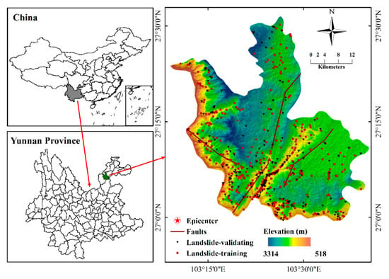
Figure 1.
Location of the study area.
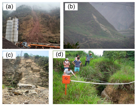
Figure 2.
(a) Slope failure, (b) debris flow, (c) rock fall, and (d) ground fissures after the 3 August 2014 earthquake event.
2.2. Landslide Inventory Mapping
A landslide inventory map is fundamental and crucial for landslide susceptibility mapping. In this study, an inventory that consists of 621 landslide sites was developed using aerial photos and Google Earth images after the 3 August 2014 earthquake event, as shown in Figure 1. To examine and confirm this inventory, all the landslide records were verified through field investigations. Of these, 435 (70%) landslides were randomly selected as the training set, and the other 186 (30%) landslides were used for validation. Additionally, we randomly selected the same number of non-landslide sites (435 and 186) from the landslide-free area to balance the whole samples for constructing training and the validation set. Note that the inventory is compiled as a point shapefile format with ArcGIS 10.5.
2.3. Landslide Conditioning Factors
The approaches for mapping landslide susceptibility require a combination of various factors indicating features of the topography, geology, and other contributing indices. The conditioning factors should also be selected according to some circumstances, such as the triggering factor and the attribute of the study area. In this study, the PGA is considered a geophysical factor contributing to landslides. The other conditioning factors are divided into topographic indices (elevation, slope, aspect, curvature, and relative relief); geology indices (lithology and distance to faults); land cover/land use (land use, normalized difference vegetation index, and the distances to roads); and hydrological indices (topographic wetness index, stream power index, and the distances to rivers). All the factors are prepared in raster format with ArcGIS 10.5.
2.3.1. Topographic Factors
The digital elevation model (DEM) in the study area is obtained from the ASTER Global Digital Elevation Model. Figure 3a shows the DEM in the study area, which has a raster format with a cell size of 30 × 30 m. The elevation has a 0.1 m vertical resolution, ranging from 747 to 3314 m. The other topographic indices, including the slope angle, slope aspect, relative relief, and curvature, are derived from the DEM. Ludian County has a total area of approximately 1487 km2, 88% of which is mountainous areas.
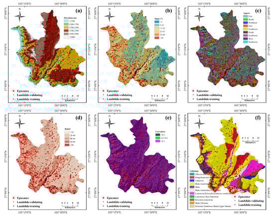
Figure 3.
Landslide conditioning factors. (a–e) Topographic factors: (a) elevation, (b) slope, (c) aspect, (d) relief, and (e) curvature); (f,g) geological factors: (f) lithology and (g) the distances to faults; (h–j) land use and land cover factors: (h) land use, (i) NDVI, and (j) the distances to roads; (k–m) hydrological factors: (k) TWI, (l) SPI, and (m) the distances to rivers; and the (n) geophysical factor: PGA.
A large slope inevitably increases the driving forces associated with gravity and the probability of landslide occurrence. Therefore, the slope is one of the most important factors in landslide susceptibility mapping. In the study area, the slope ranged from 1.2 to 75.4° (Figure 3b).
The aspect is identified as the direction of the maximum slope (Figure 3c). The soil moisture and hydrology processes are correlated with the aspect, which affects exposure to sunlight, rainfall (degree of saturation), and drying winds.
Relative relief is also a frequently used factor in LSM. Normally, the slopes with larger values of relative relief are more likely to lose stability due to earthquakes or rainfall events. Figure 3d shows the land relative relief in the study area.
The curvature is a widely used topographic factor that portrays the surface shape and changes of the slope angle. As the curvature controls the erosion process, it exerts an effect on the transport and erosion of landslide materials [36]. Negative, zero, and positive curvatures represent concave, flat, and convex shapes, respectively. In this study, the curvature was derived from the DEM and classified into three classes: <−0.1, −0.1–0.1, and >0.1 (Figure 3e).
2.3.2. Geological Factors
According to previous studies, geology plays a major role in mapping landslide susceptibility. In this study, the original lithology from a geological map was provided by the local authorities with a 1:50,000 scale, which was classified into 11 groups (in Figure 3f).
The distances to the faults were also a crucial factor to generate a landslide susceptibility map. Ludian County comprises many rocks with fractures, and they are crushed and even partly weathered, which can raise the possibility of landslides. From the fault map of the study area (Figure 3g), northeast-trending faults dominate this region. The factor of the distances to faults was divided into six groups, with values of <500 m, 500–1000 m, 1000–1500 m, 1500–2000 m, 2000–3000 m, and >3000 m.
2.3.3. Land Use and Land Cover Factors
Land use is another common factor contributing to landslides. Different soil types have different shear strengths and hydraulic conductivity, which influence the slope stability. For instance, woody vegetation can raise the stability of slopes by root reinforcement and so do manmade slopes, which have the same effects on increasing the shear strength of soil. In this study, the land use distribution (Figure 3h) was obtained from Landsat 8 using ENVI software.
Normalized difference vegetation index (NDVI) is an indicator concerned with the slope stability and has received great attention. In this study, the NDVI was obtained from the Landsat 8 image using the digital image processing (DIP) technique. The value of the NDVI is calculated as:
where R and NIR are the red portion of the electromagnetic spectrum and the infrared value, respectively. Figure 3i shows that the NDVI is classified into five groups: (<0.1, 0.1–0.2, 0.2–0.3, 0.3–0.4, and >0.4.
Roads may also affect the stability of a slope nearby, due to evacuation processes or the disruption of draining soil water. Figure 3j shows the distances to the roads in Ludian.
2.3.4. Hydrological Factors
The topographic wetness index (TWI) is a hydrological factor and has been widely used to produce landslide susceptibility maps. It is defined as follows:
where β is the slope gradient (radian), and α is the specific catchment area (m2·m−1). Figure 3k shows that the TWI is classified into six groups: <−17, −17~−15, −15~−12, −12~−8, −8~−3, and −2–11.
The Stream Power Index (SPI) is another hydrological factor that measures the erosive power of the stream. Similar to the curvature factor, the SPI may control the probability of a landslide occurrence. In this study, the SPI was divided into four groups: <15, 15–30, 30–45, and >45 (Figure 3l).
The stability of a slope around a river will be significantly affected by the fluctuation of the water in the river. Therefore, the distances to rivers are important indicators of the slope stability. In this study, the distances to rivers were classified into <300 m, 300–600 m, 600–900 m, 900–1200 m, 1200–1500, and >1500 m (Figure 3m).
2.3.5. Geophysical Factor
The peak ground acceleration (PGA) is a very important indicator for describing the strong ground motion and evaluating the earthquake intensity [37]. In general, there is a correlation between the ground motion and the occurrence of an earthquake-induced landslide, which could be useful for mapping the landslide susceptibility in earthquake-related areas [38]. In the present study, the PGA data was derived from the peak ground motion amplitudes recorded in 62 strong motion stations, with the interpolation based on estimated amplitudes where data are lacking and considering the site amplification effects [39]. The values of the PGA range from 0.06 to 0.5 g (Figure 3n).
3. Methodology
The methodological workflow in the present study is shown in Figure 4.
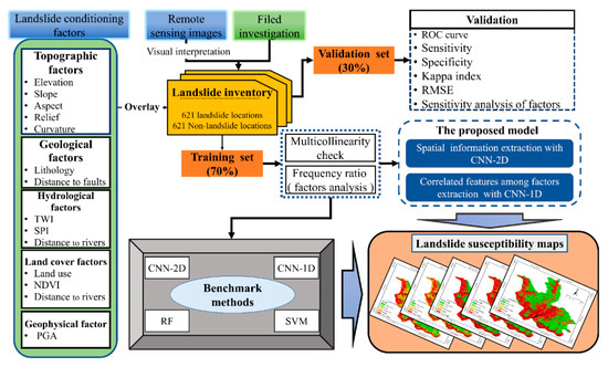
Figure 4.
The flowchart used in this research.
3.1. Conditioning Factors Analysis
The analysis and selection of the conditioning factors are very important in landslide susceptibility mapping. The number of landslide conditioning factors and their combinations significantly affect the predictive ability of susceptibility models. Indeed, the accuracy of the model does not always improve as the dimensionality of the features increase, which is known as the phenomenon of the curse of dimensionality [40]. Meanwhile, the redundancy of datasets, including excessive factors, may complicate the prediction process. Therefore, proper feature analysis and selection methods should be executed to solve these problems. In this study, two feature analysis techniques of a multicollinearity analysis and the frequency ratio are introduced in the following subsections.
3.1.1. Multicollinearity Analysis
In LSM studies, multicollinearity refers to a statistical phenomenon that describes an erroneous system analysis due to a high correlation between non-independent conditioning factors [41]. The variance inflation factors (VIF) and tolerance analysis are commonly used to check and quantify the multicollinearity among all the factors. In this analysis, let denote the set of conditioning factors and define the coefficient of determination for the regression of the conditioning factors, , on all the other conditioning factors. The formulas about the VIF and tolerance are as follows:
when the tolerance value < 0.1 or VIF > 10, it indicates the existence of multicollinearity among the conditioning factors and factors in the range the indicator value should be removed.
3.1.2. Frequency Ratio Method
The FR model is a simple but effective probability method commonly adopted to analyze the relationship between the distribution of a landslide and each landslide conditioning factor. The FR is not only the ratio of the area where a landslide occurred in the total study area but, also, the ratio of the probability of a landslide occurrence to a nonoccurrence for a given attribution [42]. The larger the FR value, the higher the probability of a landslide occurrence. In this study, the FR model was employed to reassign the categories of the conditioning factors described in Section 2.3. The FR can be calculated as:
where a is the number of each factor’s landslide, b is the number of total landslides, c is the number of pixels in a given factor, and d is the total number of total pixels in the study area.
3.2. Convolutional Neural Networks
A CNN is a type of feed-forward neural network that shows robust performances in many image classification and pattern recognition tasks [43,44]. The main distinction between a CNN and a normal neural network is that a CNN benefits from the properties of the local connective, shared weights, hierarchical features, and pooling [45]. One of the most attractive characteristics of a CNN is that it can automatically extract the hidden features from the input data. A typical CNN architecture consists of a convolutional layer, max-pooling, fully connected layer, and output layer, which are shown in Figure 5. Among them, the convolutional layer is the key part that directly contributes to the extraction of features. Using image classification as an example, the output value at the pixel (i,j) of the input x with a convolutional operator is computed as follows:
where w and n denotes the filter and its size, respectively. is the nonlinear activation function.
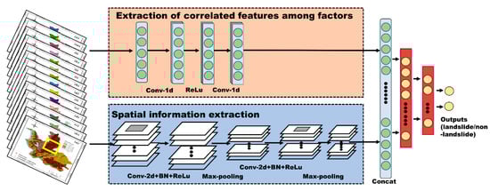
Figure 5.
The structure of the proposed model.
As the network structure deepens, more feature maps will be generated, and the parameters they carry will dramatically increase the computational cost. To solve this problem, the max-pooling operator, which is designed to reduce the size of feature maps, is introduced and defined as follows:
where is the maximum values within the filter range to the former layer. Subsequently, the feature maps extracted in the convolutional and max-pooling layers are flattened and fed into the fully connected layers (i.e., regular artificial neural network). In the following output layer, the probability that the input data belong to the corresponding class is calculated, and finally, the classification is realized. Training is performed until the model converges, and all parameters in the CNN are determined using backpropagation and gradient descent algorithms.
3.3. Proposed Model
The proposed hybrid model aims to capture the hidden but useful information automatically from the landslide inventory using the CNN architecture. First, the landslide datasets should be properly organized before being fed into the CNN-based model. In the work of reference [26], the landslide factors were stacked together and regarded as a “multi-channel image” to meet the need of the CNN input. Similarly, in the present study, we consider the landslide inventory as a “multi-spectral remote sensing data” that contains the spatial and spectral information. Here, “spatial” refers to the spatial property of a landslide as the natural hazards, and “spectral” describes the correlated features among each conditioning factor that contributes to a landslide. All the landslide conditioning factors mentioned in Section 2.3 are stacked pixel-to-pixel into 14-band spectral data. Then, as is operated in the hyperspectral remote sensing-related literature [46,47,48,49], the CNN architecture is used to extract the landslide features from both the spectral and spatial dimensions. Figure 5 shows the structure of the proposed hybrid model, which contains three parts: spatial feature extraction, spectral feature extraction, and feature fusion.
In the spatial feature extraction part, the pixel window, where all the pixels centered on the landslide point in a certain range and expand outward, is introduced to process the prepared “multi-spectral data”. Each sample is in the form of a 14 × n × n tensor, where 14 and n refer to the number of conditioning factors and the size of pixel window, respectively. Based on a large number of experiments, the n was set to 13. Theoretically, the application of a pixel window can not only capture the environmental information of the landslide location but also consider the surrounding environment around the landslide [32], which can be seen as a spatial dimension. Then, the spatial feature extraction was performed on the tensor corresponding to the landslide samples using 2D convolutional kernels, and a series of landslide feature maps at a high level was obtained.
In terms of spectral feature extraction, the conditioning factors contained in the landslide location are treated as feature vectors of the shape N × 1, where N is the number of factors. These feature vectors are generally called one-dimensional tensors in the deep learning framework. Then, a set of 1D convolutional manipulations in the CNN structure can capture the significant local representation among the landslide factors.
Having the spatial and spectral features, the next step is to fuse these features to gain a better capability of learning the pattern relationship between a landslide and the environmental variables. The landslide feature vectors and 2D feature maps are stitched together and then reorganized through fully connected layers. Finally, the fully connected layer like a binary classifier can calculate the probability of a landslide occurrence.
3.4. Evaluation and Comparison Methods
In order to evaluate the validity of the proposed model, six statistical measures were chosen, such as the area under the receiver operating characteristic curve (AUROC), Sensitivity, Specificity, Accuracy, Root mean squared error (RMSE), and Kappa index, as is shown in Equations (9)–(15). The AUROC value is a quantitative indicator of the ROC curve ranging from 0.5 to 1. An AUROC value close to 1 indicates predictions equivalent to perfect, whereas a value of 0.5 is considered a random prediction. The Sensitivity is the ratio of landslide samples that are correctly classified as landslide locations. The Specificity is the ratio of non-landslide samples that are correctly classified as non-landslide locations. The Accuracy denotes the ratio of the number of correctly classified samples to the total number of landslides and non-landslides. The RMSE is a frequently used statistical metric that measures the differences between the actual and predicted values. The Kappa index is applied to measure the reliably of the landslide susceptibility models, and its detailed description can be found in the work of reference [50].
where P and N denote the number of landslide and non-landslide samples, and TP (true positive) and TN (true negative) mean the number of landslide and non-landslide samples correctly classified, respectively. FP (false positive) and FN (false negative) mean the number of samples that are misclassified, n is the total samples in the prepared dataset, is the predicted value in the dataset, and is the actual value corresponding to the predicted value. is the expected agreement.
Besides, a support vector machine (SVM) and random forest (RF) were used as the benchmark methods to further validate the performance of the proposed model. A SVM based on the structural risk minimization principle has been widely used as an adaptable classifier to solve the binary classification in landslide susceptibility mapping [51,52]. RF is another robust classification technique and belongs to ensemble algorithms based on the bagging theory [53].
3.5. Sensitivity Analysis of Conditioning Factors
After modeling the landslide susceptibility, the critical step is to run a sensitivity analysis on the conditioning factors for quantifying their effects on the modeling results and assisting in understanding the relative importance of each factor. In the present study, a Jackknife-based test was implemented by relying on the AUC of the proposed model. The relative decrease of the AUC (RD) was calculated by comparing the results based on all the conditioning factors, so that one factor being eliminated is the indicator of importance [54]. The higher the RD of a conditioning factor is, the more contribution it has to the susceptibility model. The formula for the RD is as follows:
where AUCall and AUCi represent the AUC computed from the prediction using all the fac-tors and the prediction without using the ith factor, respectively.
4. Results
4.1. Selection and Analysis of the Landslide Conditioning Factors
In this subsection, a multicollinearity analysis and FR model were applied for the selection and analysis of those conditioning factors. Table 1 lists the results of the collinearity analysis under the condition of a 95% confidence level. It can be observed that the highest VIF value is 3.488 (slope), and the lowest TOL is 0.287 (slope). This result is not within the critical range of the existence of the multicollinearity, which indicated that all the conditioning factors were independent, and there was no multicollinearity among them.

Table 1.
Variance inflation factors (VIF) and tolerances of each conditioning factor.
Figure 6 summarizes the correlations between landslides and each conditioning factor. As this method previously mentioned, the magnitude of probability of a landslide occurrence can be inferred from the FR value. For elevation, the class of 1300–1700 m has the highest FR value, indicating the highest probability of a landslide occurrence. The result of the slope revealed that most landslides occurred in 25–35° and 35–45° (1.58 and 1.44, respectively). The TWI result demonstrated that the −8~−3 class has a significantly higher FR value than the other classes, with a value of 3.07, which indicated the highest probability of a landslide occurrence. For the SPI factor, the >45 class had the highest RF value of 1.42, followed by the <15 class with a FR value of 0.98. Interestingly, some factors showed a clear spatial distribution upon the FR results. For example, the FR values of the <300 m class of the distances to the rivers and the <400 m class of the distances to the roads were much higher than the other classes, which indicated that landslides occurred close to rivers and roads. The FR value of the NDVI decreased as the uprooted vegetation increased. In the case of the PGA, the FR values increased with the increasing PGA values, as expected. The highest FR value (that is, a representation of a high probability regarding landslide occurrences) belonged to the 0.30–0.38 class, which can reflect the correlation between the distribution of landslides and ground shaking. For the curvature factor, the −0.1–0.1 (flat) class had the lowest FR value, indicating the lowest probability of a landslide occurrence in the flat area, which was not only consistent with the general knowledge on landslides but also confirmed the reliability of the dataset in this work. However, for the factors of lithology, the distances to faults, relief, and aspect, there was not a clear distinction between the classes’ FR value. After these analyses, we reassigned the factors classification described in Section 2.3 based on the FR values and normalized them to 0–1.
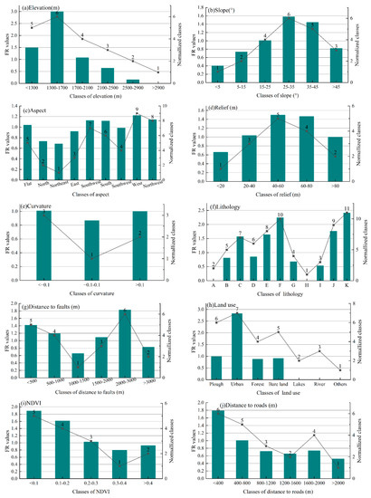
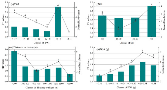
Figure 6.
Relationship between the landslides and the conditioning factors: (a) Elevation (m), (b) Slope (°), (c) Aspect, (d) Relief (m), (e) Curvature, (f) Lithology, (g) the distances to the faults (m), (h) land use, (i) the NDVI, (j) the distances to the roads (m), (k) TWI, (l) SPI, (m) the distances to the rivers (m), and (n) the PGA.
4.2. Construction of Proposed Model
The preprocessed data in terms of the tensor was fed into the hybrid model that was described in Section 3.3. This hybrid model contained two input nodes and one output node. One of the input nodes corresponded to the spatial information extraction part, where the pixel window data were fed. A series of feature maps were generated through two 2D convolutional layers and two max-pooling layers, and these maps were then stretched into one-dimensional tensors by flatten manipulation. The other node was linked to the block of spectral information extraction. The input data of this block was one-dimensional tensor data reflecting an implicit relationship between the landslide factors. Given the sparsity and length of the 1D input data, we only used two 1D convolutional layers in this part without embedding a pooling layer. It should be noted that the two blocks of the model were trained synchronously in each epoch, which guaranteed the consistency of the training parameters.
Model hyperparameters generally exert a strong impact on the performance of machine learning methods; thus, it is necessary to execute a tuning process before model training [55]. In this work, all the hyperparameters of the hybrid model, including the numbers and sizes of the filters, batch sizes, activation functions, optimizers, and the neurons in the hidden layers, were determined based on a five-fold cross-validation, as shown in Table 2. Figure 7 shows the training losses and accuracies over 300 epochs using backpropagation and gradient descent algorithms. It can be seen that the model accuracy shows fluctuations at the early stage; then, it increases over time and finally stabilizes after approximately 300 epochs. A similar trend was shown in the model loss, which suggested that the model converged. In other words, the model we obtained learned an implicit correlation between a landslide and its environmental conditions.
Table 2.
Hyperparameters of the proposed model.
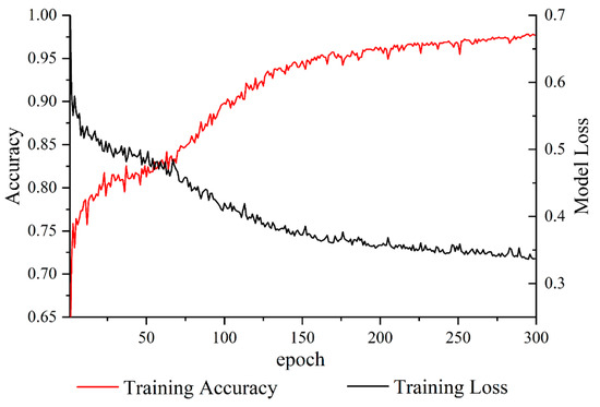
Figure 7.
Training curves of the proposed model.
With regards to the runtime environment, the hybrid CNN-based model proposed in this study was developed in python using Pytorch, a deep learning framework package, on a computer with 2.9 GHz Intel(R) Core (TM) i5-10400F CPU, a 6 GB graphic card GTX1660s, and 16 GB of RAM.
4.3. Generation of Landslide Susceptibility Maps
The trained hybrid model was used to prepare the landslide susceptibility map by calculating the probability of a landslide occurrence of each pixel, and the susceptibility values were reclassified into five different degrees with the help of the natural break technique in ArcGIS 10.5—namely, very low (VL), low (L), moderate (M), high (H), and very high (VH), as shown in Figure 8a. It can be observed that the VH zone derived using the hybrid model covered 44.1% of the total area, 38.1%, 6.4%, 5.0%, and 6.3% of the total area belonging to the VL, L, M, and H zones, respectively. Figure 8b–e illustrated the LSM of the RF, SVM, and two basic CNN models. For 1D-CNN and 2D-CNN models, a susceptibility distribution similar to that of the hybrid model observed that most of area was classified as VH and VL zones; in contrast, the rest of susceptibility zones only occupied a small portion. However, in the case of the RF model, the areal coverage in percentage for the VH zone was 18.4%. The H, M, L, and VL zones accounted for 20.0%, 21.1%, 22.2%, and 18.3% of the study area, respectively. According to the SVM model, 17.3%, 19.6%, 21.3%, 18.3%, and 22.6% of the study area were designated to be of the VH, H, M, L, and VL zones, respectively.
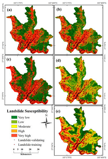
Figure 8.
Landslide susceptibility maps using (a) a hybrid model, (b) CNN-2D, (c) CNN-1D, (d) RF, and (e) SVM.
Interestingly, as shown in Table 3, the three CNN-based models provided a classification that sharply divided the VH zone from relative low zones, while the conventional machine learning (ML)-based model showed stable classification results of each susceptibility zone, which demonstrated the significant sensitivity of the CNN-based models to the VH and VL zones. These results can be explained by the entire calculation process of susceptibility. In general, a trained model with good predictive ability can determine, in terms of probability values, how likely a landslide is to occur in each target pixel. As shown in Figure 8, the LSM that reflects different susceptibility zones essentially responds to the resultant probability values. CNN-based models are capable of extracting more spatial information better than conventional ML methods, which allows them to learn sufficient landslide features from training samples without excessive noise. Therefore, the probability values computed by CNN-based models tend to be two extreme values: ~1 and ~0, while those computed by conventional ML methods are arbitrarily distributed from 0 to 1.
Table 3.
Area (km2) of each susceptibility class.
4.4. Evaluation and Comparison of Results
In this subsection, the validation and comparison processes were performed according to the predicted results and the observed landslide. Figure 9 illustrates the relationship between the landslide susceptibility zones and the density of the observed landslides. It can be seen that the landslide density of the VH zone was the maximum, followed by the H, M, L, and VL zones, respectively. It was evident that the proposed model correctly predicted most of the observed landslides in the VH susceptibility zone.
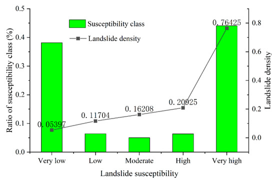
Figure 9.
Landslide density of the various susceptibility classes of LSM generated by the proposed model.
The AUC value estimated using the ROC curve provided a direct comparison of the different models. As shown in Figure 10, the maximum AUC (89.6%) in the validation set was obtained for the proposed hybrid model and followed by CNN-1D (85.9%), RF (83.6%), CNN-2D (83.4%), and SVM (81.3%). These results indicated that the proposed model was the best-performing model for predicting landslide occurrences in comparison to the four benchmark models. Specifically, the AUC of the proposed hybrid model was 6.2% and 3.7% higher than the pure CNN-2D and CNN-1D models, respectively.
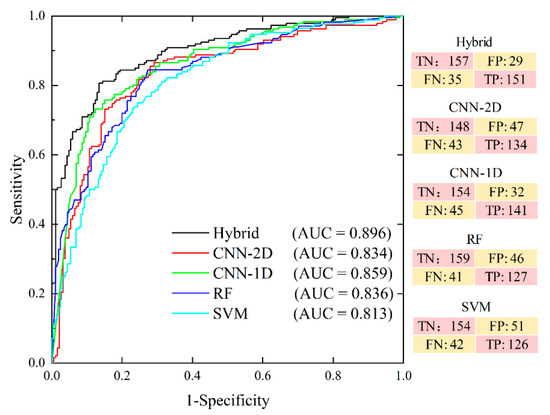
Figure 10.
The receiver operating characteristic (ROC) curves on the validation set (with a confusion matrix where the TN, FP, FN, and TP denote the true negative, false positive, false negative, and true positive, respectively).
Figure 11 shows the Accuracy, Sensitivity, Specificity, Kappa, and RMSE values of the proposed hybrid model and four benchmark models in the validation set. It can be seen that the proposed hybrid model achieved the best results compared to the other four benchmark models. In terms of Sensitivity, the proposed hybrid model achieved the highest Sensitivity value of 81.1%, which was approximately 5% higher than that of the CNN-1D model (75.8%), followed by CNN-2D, RF, and SVM, respectively. These results demonstrated that the proposed hybrid model showed a better performance in correctly classifying the landslide samples as landslide locations compared with the four benchmark models. A similar result was also observed in the Specificity values, which indicated that the proposed hybrid model outperformed the others in terms of accurately classifying the non-landslide locations. In addition, the Kappa index results indicated that the proposed model (0.656) had the highest index value, followed by CNN-1D (0.596), CNN-2D (0.569), RF (0.530), and SVM (0.499).
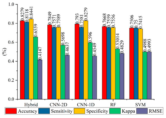
Figure 11.
Model evaluation and comparison in the validation set.
4.5. Sensitivity Analysis Results
A preliminary analysis on the relationship between the conditioning factors and landslide occurrences was presented in Section 4.1, while the effect of a single factor on the modeling results remains unclear. To tackle this, a sensitivity analysis of 14 conditioning factors based on the Jackknife test was implemented to explore the contribution (i.e., importance) of each factor to the proposed susceptibility model. Figure 12 shows the results in terms of the relative decrease of the AUC values. It can be observed that the three most important factors are elevation, PGA, and slope, respectively. The elevation has the highest RD value of ~7% when eliminated in the proposed model, which demonstrated a high contribution to the modeling results. The second most influential factor was the PGA, which got an RD value of 5.9%. Numerous studies have demonstrated that there is a high correlation between the occurrence of co-seismic landslides and PGA [38,56]. Our study confirmed that the PGA factor should be considered for mapping the earthquake-induced landslide susceptibility. Besides, it is worth noting that the factor of the distances to the faults that sometimes used to substitute the effects of earthquakes did not show a high RD value compared with the PGA. One possible reason for this result is that earthquakes are not always triggered by fault activities, as reported by Chang et al. [57]. Overall, all the factors used in this study contributed to the modeling results, but the importance of the related landslide conditioning factors still needs to be explored in different study areas.
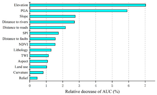
Figure 12.
Sensitivity analysis results based on the Jackknife test.
5. Discussion
Landslide is one of the most widespread natural hazards around the world, causing incalculable casualties and economic losses, as well as damage to the landscapes of landslide-prone areas. Over the past years, various methods and technical frameworks have been applied for landslide hazard management and mitigation, covering identification, susceptibility mapping, and monitoring. Of them, landslide susceptibility mapping (LSM) plays an important role in providing a thematic map for portraying where landslides are likely to occur and the probability of their occurrence. A landslide inventory consisting of landslide points and related conditioning factors is the basis of LSM, but the number of landslide points is usually restricted due to the time-consuming and labor-intensive collection process [33]. The motivation of this study is to capture more landslide representation from a limited dataset. To achieve this goal, we selected the convolutional neural network as the basic module and proposed a hybrid model that integrates the spatial information and the correlated features among the conditioning factors, offering a synergistic opportunity for them.
In previous related literature, the hybrid model was considered to improve the landslide predictive capability by reducing the variance and bias [58,59]. In our experiments, the proposed hybrid model achieved the best performance in terms of the AUC value and the other statistical measures compared with the four benchmark models. These results, to some extent, met the expectations of the hybrid model and can be considered promising. Meanwhile, the overall performances of the three CNN-based models (i.e., hybrid, CNN-2D, and CNN-1D) were significantly higher than that of the conventional machine learning models (i.e., RF and SVM), since CNN-based models have a complicated architecture that enhances their capability of capturing landslide representations from high levels using convolution and pooling operations. [60]. Furthermore, among the three CNN-based models, the proposed hybrid method showed a higher performance than any of the single 1D- or 2D-CNN models, as shown in Figure 10 and Figure 11. This is reasonable, because the hybrid model enhanced the landslide prediction accuracy effectively by extracting spatial information and correlated information among the landslide conditioning factors from the landslide inventory. Put simply, more landslide-related representations were captured from the limited datasets when using the proposed hybrid model.
Despite the excellent feature extraction capability of a CNN, an overfitting problem, which needs to be avoided, usually occurs due to the conflict between the complicated structure and insufficient landslide samples. To further check how the models fit, we plotted the ROC curve on the training set, which is also called the success rate curve (SRC), as shown in Figure 13. Figure 10 and Figure 13 show that the CNN-2D had the highest AU-SRC value of ~1, while its AUC value on the validation set was smaller than that of the proposed model, which indicated the existence of a somewhat overfitting risk in the CNN-2D model. The structure of the proposed hybrid model was significantly more complex than that of the pure CNN models but effectively avoided the overfitting risk. Therefore, it seems reasonable that the proposed model is capable of extracting more landslide information from the limited landslide samples by generating additional data from the original dataset, as reported in the previous studies of hybrid model [61,62,63].
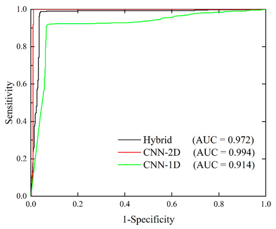
Figure 13.
The receiver operating characteristic (ROC) curves on the training set.
In addition, the susceptibility maps can, in turn, reflect the reasonableness and reliability of the models. As shown in Figure 8, most landslides fell into the VH susceptibility zone in the LSM of the three CNN-based models. This result is a positive sign from a disaster mitigation perspective view, because it means that the built models are capable of precisely calculating the probability of a landslide occurrence and providing safe hazard mitigation measures to decision-makers. Besides, researchers also use the Specificity and Sensitivity indices to further assess the reliability of a susceptibility model. A susceptibility model with a high Specificity value may avoid economic losses, since it can correctly classify non-landslide areas as stable slopes and maximize the use of the landscape. Additionally, a model with a high Sensitivity value can provide safe mitigation guidance due to accurately identifying landslide-prone areas [10,64]. In the present study, both the Specificity and Sensitivity values of the proposed model in the validation set were higher than the other benchmark models, thus proving reliability for hazard mitigation and land use planning.
6. Conclusions
In the present work, a robust CNN-based hybrid model that incorporates the spatial representations of the conditioning factors with the correlated information between the factors was proposed and successfully applied to map the landslide susceptibility in Ludian County, China. The experiment results showed that the proposed hybrid model achieved the highest performance for predicting the landslide occurrence compared to the four benchmark methods of CNN-1D, CNN-2D, RF, and SVM. Specifically, the AUC of the proposed hybrid model was 4.7% and 5.9% higher than the pure CNN-2D and CNN-1D models, respectively. Additionally, the overall performances of the three CNN-based models were somewhat higher than that of the conventional machine learning methods in terms of the AUC, which indicated the remarkable features extraction capability of the CNN. The results also demonstrated that the proposed model effectively avoided an overfitting risk by generating additional data from the limited dataset. Moreover, the proposed hybrid model with high Specificity and Sensitivity values confirmed its reliability and safety for hazard mitigation. A Sensitivity analysis of the conditioning factors to the proposed hybrid model showed that the elevation, PGA, and slope made strong contributions to the modeling results. Based on all the results and discussion, conclusions can be drawn that the proposed hybrid model effectively enhanced the capability of mapping the landslide susceptibility and provided a reliable and promising tool for hazard mitigation and land use planning. However, the performance of the proposed model needs to be further tested in additional research and case studies.
Author Contributions
Conceptualization, X.Y. and R.L.; software and coding, X.Y.; formal analysis, T.L. and J.C.; data curation, M.Y., Y.Y. and Y.W.; writing—original draft, X.Y.; writing—review and editing, X.Y., R.L., M.Y., J.C., W.C. and Y.W.; project administration, R.L.; and funding acquisition, R.L. All authors have read and agreed to the published version of the manuscript.
Funding
This research was funded by the Bureau of Geology and mineral resources exploration and development of Sichuan Province, grant number 20170612-0413 and China Geological Survey, grant number 1512007402438.
Institutional Review Board Statement
Not applicable.
Informed Consent Statement
Not applicable.
Data Availability Statement
Data sharing is not applicable to this article.
Acknowledgments
The authors would like to express their sincere thanks to the handling editors and the two anonymous reviewers, as their valuable comments and suggestions greatly improved the quality of the paper. The authors also would like to thank Kun Chen from the Institute of Geophysics, China Earthquake Administration for sharing the PGA data. In addition, Xin Yang wants to thank, in particular, the care and support from Mengtian Li during the COVID-19 epidemic.
Conflicts of Interest
The authors declare no conflict of interest.
References
- Tsangaratos, P.; Ilia, I. Comparison of a logistic regression and Naïve Bayes classifier in landslide susceptibility assessments: The influence of models complexity and training dataset size. Catena 2016, 145, 164–179. [Google Scholar] [CrossRef]
- Hassangavyar, M.B.; Damaneh, H.E.; Pham, Q.B.; Linh, N.T.T.; Tiefenbacher, J.; Bach, Q.-V. Evaluation of re-sampling methods on performance of machine learning models to predict landslide susceptibility. Geocarto Int. 2020, 1–23. [Google Scholar] [CrossRef]
- Samia, J.; Temme, A.; Bregt, A.; Wallinga, J.; Guzzetti, F.; Ardizzone, F.; Rossi, M. Do landslides follow landslides? Insights in path dependency from a multi-temporal landslide inventory. Landslides 2016, 14, 547–558. [Google Scholar] [CrossRef]
- Hess, D.M.; Leshchinsky, B.A.; Bunn, M.; Benjamin Mason, H.; Olsen, M.J. A simplified three-dimensional shallow landslide susceptibility framework considering topography and seismicity. Landslides 2017, 14, 1677–1697. [Google Scholar] [CrossRef]
- Özdemir, A.; Delikanli, M. A geotechnical investigation of the retrogressive Yaka Landslide and the debris flow threatening the town of Yaka (Isparta, SW Turkey). Nat. Hazards 2008, 49, 113–136. [Google Scholar] [CrossRef]
- Chen, X.-L.; Liu, C.-G.; Wang, M.-M.; Zhou, Q. Causes of unusual distribution of coseismic landslides triggered by the Mw 6.1 2014 Ludian, Yunnan, China earthquake. J. Asian Earth Sci. 2018, 159, 17–23. [Google Scholar] [CrossRef]
- Li, W.-L.; Huang, R.-Q.; Tang, C.; Xu, Q.; van Westen, C. Co-seismic landslide inventory and susceptibility mapping in the 2008 Wenchuan earthquake disaster area, China. J. Mt. Sci. 2013, 10, 339–354. [Google Scholar] [CrossRef]
- Tian, Y.; Xu, C.; Ma, S.; Xu, X.; Wang, S.; Zhang, H. Inventory and Spatial Distribution of Landslides Triggered by the 8th August 2017 MW 6.5 Jiuzhaigou Earthquake, China. J. Earth Sci. 2018, 30, 206–217. [Google Scholar] [CrossRef]
- Yang, Z.-H.; Lan, H.-X.; Gao, X.; Li, L.-P.; Meng, Y.-S.; Wu, Y.-M. Urgent landslide susceptibility assessment in the 2013 Lushan earthquake-impacted area, Sichuan Province, China. Nat. Hazards 2014, 75, 2467–2487. [Google Scholar] [CrossRef]
- Jaafari, A.; Panahi, M.; Pham, B.T.; Shahabi, H.; Bui, D.T.; Rezaie, F.; Lee, S. Meta optimization of an adaptive neuro-fuzzy inference system with grey wolf optimizer and biogeography-based optimization algorithms for spatial prediction of landslide susceptibility. Catena 2019, 175, 430–445. [Google Scholar] [CrossRef]
- Reichenbach, P.; Rossi, M.; Malamud, B.D.; Mihir, M.; Guzzetti, F. A review of statistically-based landslide susceptibility models. Earth Sci. Rev. 2018, 180, 60–91. [Google Scholar] [CrossRef]
- Constantin, M.; Bednarik, M.; Jurchescu, M.C.; Vlaicu, M. Landslide susceptibility assessment using the bivariate statistical analysis and the index of entropy in the Sibiciu Basin (Romania). Environ. Earth Sci. 2010, 63, 397–406. [Google Scholar] [CrossRef]
- Chen, X.; Chen, W. GIS-based landslide susceptibility assessment using optimized hybrid machine learning methods. Catena 2021, 196. [Google Scholar] [CrossRef]
- Panchal, S.; Shrivastava, A.K. Application of analytic hierarchy process in landslide susceptibility mapping at regional scale in GIS environment. J. Stat. Manag. Syst. 2020, 23, 199–206. [Google Scholar] [CrossRef]
- Moragues, S.; Lenzano, M.G.; Lanfri, M.; Moreiras, S.; Lannutti, E.; Lenzano, L. Analytic hierarchy process applied to landslide susceptibility mapping of the North Branch of Argentino Lake, Argentina. Nat. Hazards 2020, 105, 915–941. [Google Scholar] [CrossRef]
- Dahal, R.K.; Hasegawa, S.; Nonomura, A.; Yamanaka, M.; Masuda, T.; Nishino, K. GIS-based weights-of-evidence modelling of rainfall-induced landslides in small catchments for landslide susceptibility mapping. Environ. Geol. 2007, 54, 311–324. [Google Scholar] [CrossRef]
- Li, L.; Lan, H.; Guo, C.; Zhang, Y.; Li, Q.; Wu, Y. A modified frequency ratio method for landslide susceptibility assessment. Landslides 2016, 14, 727–741. [Google Scholar] [CrossRef]
- Shafapour Tehrany, M.; Kumar, L.; Neamah Jebur, M.; Shabani, F. Evaluating the application of the statistical index method in flood susceptibility mapping and its comparison with frequency ratio and logistic regression methods. Geomat. Nat. Hazards Risk 2018, 10, 79–101. [Google Scholar] [CrossRef]
- Zhang, T.-Y.; Han, L.; Zhang, H.; Zhao, Y.-H.; Li, X.-A.; Zhao, L. GIS-based landslide susceptibility mapping using hybrid integration approaches of fractal dimension with index of entropy and support vector machine. J. Mt. Sci. 2019, 16, 1275–1288. [Google Scholar] [CrossRef]
- Chen, W.; Pourghasemi, H.R.; Kornejady, A.; Zhang, N. Landslide spatial modeling: Introducing new ensembles of ANN, MaxEnt, and SVM machine learning techniques. Geoderma 2017, 305, 314–327. [Google Scholar] [CrossRef]
- Liu, R.; Li, L.; Pirasteh, S.; Lai, Z.; Yang, X.; Shahabi, H. The performance quality of LR, SVM, and RF for earthquake-induced landslides susceptibility mapping incorporating remote sensing imagery. Arabian J. Geosci. 2021, 14. [Google Scholar] [CrossRef]
- Xu, C.; Xu, X.; Dai, F.; Saraf, A.K. Comparison of different models for susceptibility mapping of earthquake triggered landslides related with the 2008 Wenchuan earthquake in China. Comput. Geosci. 2012, 46, 317–329. [Google Scholar] [CrossRef]
- Kumar, D.; Thakur, M.; Dubey, C.S.; Shukla, D.P. Landslide susceptibility mapping & prediction using Support Vector Machine for Mandakini River Basin, Garhwal Himalaya, India. Geomorphology 2017, 295, 115–125. [Google Scholar] [CrossRef]
- Tien Bui, D.; Pradhan, B.; Lofman, O.; Revhaug, I.; Dick, O.B. Landslide susceptibility mapping at Hoa Binh province (Vietnam) using an adaptive neuro-fuzzy inference system and GIS. Comput. Geosci. 2012, 45, 199–211. [Google Scholar] [CrossRef]
- Pham, V.D.; Nguyen, Q.-H.; Nguyen, H.-D.; Pham, V.-M.; Vu, V.M.; Bui, Q.-T. Convolutional Neural Network—Optimized Moth Flame Algorithm for Shallow Landslide Susceptible Analysis. IEEE Access 2020, 8, 32727–32736. [Google Scholar] [CrossRef]
- Wang, Y.; Fang, Z.; Hong, H. Comparison of convolutional neural networks for landslide susceptibility mapping in Yanshan County, China. Sci. Total Environ. 2019, 666, 975–993. [Google Scholar] [CrossRef] [PubMed]
- Chen, Y.; Ming, D.; Ling, X.; Lv, X.; Zhou, C. Landslide Susceptibility Mapping Using Feature Fusion Based CPCNN-ML in Lantau Island, Hong Kong. IEEE J. Sel. Top. Appl. Earth Obs. Remote Sens. 2021. [Google Scholar] [CrossRef]
- Xiao, L.; Zhang, Y.; Peng, G. Landslide Susceptibility Assessment Using Integrated Deep Learning Algorithm along the China-Nepal Highway. Sensors 2018, 18, 4436. [Google Scholar] [CrossRef] [PubMed]
- Wang, Y.; Fang, Z.; Wang, M.; Peng, L.; Hong, H. Comparative study of landslide susceptibility mapping with different recurrent neural networks. Comput. Geosci. 2020, 138. [Google Scholar] [CrossRef]
- Pourghasemi, H.R.; Kornejady, A.; Kerle, N.; Shabani, F. Investigating the effects of different landslide positioning techniques, landslide partitioning approaches, and presence-absence balances on landslide susceptibility mapping. Catena 2020, 187. [Google Scholar] [CrossRef]
- Dou, J.; Yunus, A.P.; Merghadi, A.; Shirzadi, A.; Nguyen, H.; Hussain, Y.; Avtar, R.; Chen, Y.; Pham, B.T.; Yamagishi, H. Different sampling strategies for predicting landslide susceptibilities are deemed less consequential with deep learning. Sci. Total Environ. 2020, 720, 137320. [Google Scholar] [CrossRef] [PubMed]
- Yi, Y.; Zhang, Z.; Zhang, W.; Jia, H.; Zhang, J. Landslide susceptibility mapping using multiscale sampling strategy and convolutional neural network: A case study in Jiuzhaigou region. Catena 2020, 195. [Google Scholar] [CrossRef]
- Zhu, Q.; Chen, L.; Hu, H.; Pirasteh, S.; Li, H.; Xie, X. Unsupervised Feature Learning to Improve Transferability of Landslide Susceptibility Representations. IEEE J. Sel. Top. Appl. Earth Obs. Remote Sens. 2020, 13, 3917–3930. [Google Scholar] [CrossRef]
- Jing-chun, X.; Rui, L.; Hui-wen, L.; Zi-li, L. Analysis of landslide hazard area in Ludian earthquake based on Random Forests. Int. Arch. Photogramm. Remote. Sens. Spat. Inf. Sci. 2015. [Google Scholar] [CrossRef]
- Zhou, J.-W.; Lu, P.-Y.; Hao, M.-H. Landslides triggered by the 3 August 2014 Ludian earthquake in China: Geological properties, geomorphologic characteristics and spatial distribution analysis. Geomat. Nat. Hazards Risk 2015, 7, 1219–1241. [Google Scholar] [CrossRef]
- Gnyawali, K.R.; Zhang, Y.; Wang, G.; Miao, L.; Pradhan, A.M.S.; Adhikari, B.R.; Xiao, L. Mapping the susceptibility of rainfall and earthquake triggered landslides along China–Nepal highways. Bull. Eng. Geol. Environ. 2019, 79, 587–601. [Google Scholar] [CrossRef]
- Douglas, J. Earthquake ground motion estimation using strong-motion records: A review of equations for the estimation of peak ground acceleration and response spectral ordinates. Earth Sci. Rev. 2003, 61, 43–104. [Google Scholar] [CrossRef]
- Huang, H.-P.; Yang, K.-C.; Lin, B.-W. Statistical evaluation of the effect of earthquake with other related factors on landslide susceptibility: Using the watershed area of Shihmen reservoir in Taiwan as a case study. Environ. Earth Sci. 2012, 69, 2151–2166. [Google Scholar] [CrossRef]
- Chen, K.; Yu, Y.X.; Gao, M.T.; Kang, C.C. ShakeMap of peak ground acceleration for 2014 Ludian, Yunnan, Ms6.5 earthquake. Acta Seismol. Sin. 2015, 429–436. [Google Scholar] [CrossRef]
- Hidalgo-Mompeán, F.; Gómez Fernández, J.F.; Cerruela-García, G.; Crespo Márquez, A. Dimensionality analysis in machine learning failure detection models. A case study with LNG compressors. Comput. Ind. 2021, 128. [Google Scholar] [CrossRef]
- Tien Bui, D.; Tuan, T.A.; Klempe, H.; Pradhan, B.; Revhaug, I. Spatial prediction models for shallow landslide hazards: A comparative assessment of the efficacy of support vector machines, artificial neural networks, kernel logistic regression, and logistic model tree. Landslides 2015, 13, 361–378. [Google Scholar] [CrossRef]
- Hong, H.; Liu, J.; Zhu, A.X. Landslide susceptibility evaluating using artificial intelligence method in the Youfang district (China). Environ. Earth Sci. 2019, 78. [Google Scholar] [CrossRef]
- Sfikas, K.; Pratikakis, I.; Theoharis, T. Ensemble of PANORAMA-based convolutional neural networks for 3D model classification and retrieval. Comput. Graph. 2018, 71, 208–218. [Google Scholar] [CrossRef]
- Ramakrishnan, S.; Muthanantha Murugavel, A.S.; Sathiyamurthi, P.; Ramprasath, J. Seizure Detection with Local Binary Pattern and CNN Classifier. J. Phys. Conf. Ser. 2021, 1767. [Google Scholar] [CrossRef]
- Lecun, Y.; Bottou, L.; Bengio, Y.; Haffner, P. Gradient-based learning applied to document recognition. Proc. IEEE 1998, 86, 2278–2324. [Google Scholar] [CrossRef]
- Guo, H.; Liu, J.; Xiao, Z.; Xiao, L. Deep CNN-based hyperspectral image classification using discriminative multiple spatial-spectral feature fusion. Remote Sens. Lett. 2020, 11, 827–836. [Google Scholar] [CrossRef]
- Shi, H.; Cao, G.; Ge, Z.; Zhang, Y.; Fu, P. Double-Branch Network with Pyramidal Convolution and Iterative Attention for Hyperspectral Image Classification. Remote Sens. 2021, 13, 1403. [Google Scholar] [CrossRef]
- He, X.; Chen, Y.; Lin, Z. Spatial-Spectral Transformer for Hyperspectral Image Classification. Remote Sens. 2021, 13, 498. [Google Scholar] [CrossRef]
- Yue, J.; Zhao, W.; Mao, S.; Liu, H. Spectral–spatial classification of hyperspectral images using deep convolutional neural networks. Remote Sens. Lett. 2015, 6, 468–477. [Google Scholar] [CrossRef]
- Chen, T.; Zhu, L.; Niu, R.-Q.; Trinder, C.J.; Peng, L.; Lei, T. Mapping landslide susceptibility at the Three Gorges Reservoir, China, using gradient boosting decision tree, random forest and information value models. J. Mt. Sci. 2020, 17, 670–685. [Google Scholar] [CrossRef]
- Vapnik, V.N. The Nature of Statistical Learning Theory; Springer: New York, NY, USA, 1995. [Google Scholar] [CrossRef]
- Islam, A.; Talukdar, S.; Mahato, S.; Ziaul, S.; Eibek, K.U.; Akhter, S.; Pham, Q.B.; Mohammadi, B.; Karimi, F.; Linh, N.T.T. Machine learning algorithm-based risk assessment of riparian wetlands in Padma River Basin of Northwest Bangladesh. Environ. Sci. Pollut. Res. Int. 2021. [Google Scholar] [CrossRef] [PubMed]
- Shirvani, Z. A Holistic Analysis for Landslide Susceptibility Mapping Applying Geographic Object-Based Random Forest: A Comparison between Protected and Non-Protected Forests. Remote Sens. 2020, 12, 434. [Google Scholar] [CrossRef]
- Park, N.-W. Using maximum entropy modeling for landslide susceptibility mapping with multiple geoenvironmental data sets. Environ. Earth Sci. 2014, 73, 937–949. [Google Scholar] [CrossRef]
- Lujan-Moreno, G.A.; Howard, P.R.; Rojas, O.G.; Montgomery, D.C. Design of experiments and response surface methodology to tune machine learning hyperparameters, with a random forest case-study. Expert Syst. Appl. 2018, 109, 195–205. [Google Scholar] [CrossRef]
- Meunier, P.; Hovius, N.; Haines, A.J. Regional patterns of earthquake-triggered landslides and their relation to ground motion. Geophys. Res. Lett. 2007, 34. [Google Scholar] [CrossRef]
- Chang, K.-T.; Chiang, S.-H.; Hsu, M.-L. Modeling typhoon- and earthquake-induced landslides in a mountainous watershed using logistic regression. Geomorphology 2007, 89, 335–347. [Google Scholar] [CrossRef]
- Fang, Z.; Wang, Y.; Duan, G.; Peng, L. Landslide Susceptibility Mapping Using Rotation Forest Ensemble Technique with Different Decision Trees in the Three Gorges Reservoir Area, China. Remote Sens. 2021, 13, 238. [Google Scholar] [CrossRef]
- Pham, B.T.; Prakash, I.; Singh, S.K.; Shirzadi, A.; Shahabi, H.; Tran, T.-T.-T.; Bui, D.T. Landslide susceptibility modeling using Reduced Error Pruning Trees and different ensemble techniques: Hybrid machine learning approaches. Catena 2019, 175, 203–218. [Google Scholar] [CrossRef]
- Sameen, M.I.; Pradhan, B.; Lee, S. Application of convolutional neural networks featuring Bayesian optimization for landslide susceptibility assessment. Catena 2020, 186. [Google Scholar] [CrossRef]
- Sameen, M.I.; Sarkar, R.; Pradhan, B.; Drukpa, D.; Alamri, A.M.; Park, H.-J. Landslide spatial modelling using unsupervised factor optimisation and regularised greedy forests. Comput. Geosci. 2020, 134. [Google Scholar] [CrossRef]
- Choubin, B.; Moradi, E.; Golshan, M.; Adamowski, J.; Sajedi-Hosseini, F.; Mosavi, A. An ensemble prediction of flood susceptibility using multivariate discriminant analysis, classification and regression trees, and support vector machines. Sci. Total Environ. 2019, 651, 2087–2096. [Google Scholar] [CrossRef] [PubMed]
- Yan, F.; Zhang, Q.; Ye, S.; Ren, B. A novel hybrid approach for landslide susceptibility mapping integrating analytical hierarchy process and normalized frequency ratio methods with the cloud model. Geomorphology 2019, 327, 170–187. [Google Scholar] [CrossRef]
- Zhou, C.; Yin, K.; Cao, Y.; Ahmed, B.; Li, Y.; Catani, F.; Pourghasemi, H.R. Landslide susceptibility modeling applying machine learning methods: A case study from Longju in the Three Gorges Reservoir area, China. Comput. Geosci. 2018, 112, 23–37. [Google Scholar] [CrossRef]


Publisher’s Note: MDPI stays neutral with regard to jurisdictional claims in published maps and institutional affiliations. |
© 2021 by the authors. Licensee MDPI, Basel, Switzerland. This article is an open access article distributed under the terms and conditions of the Creative Commons Attribution (CC BY) license (https://creativecommons.org/licenses/by/4.0/).