Hyperspectral Unmixing Based on Constrained Bilinear or Linear-Quadratic Matrix Factorization

Abstract

Unsupervised hyperspectral unmixing methods aim to extract endmember spectra and infer the proportion of each of these spectra in each observed pixel when considering linear mixtures. However, the interaction between sunlight and the Earth’s surface is often very complex, so that observed spectra are then composed of nonlinear mixing terms. This nonlinearity is generally bilinear or linear quadratic. In this work, unsupervised hyperspectral unmixing methods, designed for the bilinear and linear-quadratic mixing models, are proposed. These methods are based on bilinear or linear-quadratic matrix factorization with non-negativity constraints. Two types of algorithms are considered. The first ones only use the projection of the gradient, and are therefore linked to an optimal manual choice of their learning rates, which remains the limitation of these algorithms. The second developed algorithms, which overcome the above drawback, employ multiplicative projective update rules with automatically chosen learning rates. In addition, the endmember proportions estimation, with three alternative approaches, constitutes another contribution of this work. Besides, the reduction of the number of manipulated variables in the optimization processes is also an originality of the proposed methods. Experiments based on realistic synthetic hyperspectral data, generated according to the two considered nonlinear mixing models, and also on two real hyperspectral images, are carried out to evaluate the performance of the proposed approaches. The obtained results show that the best proposed approaches yield a much better performance than various tested literature methods.

1. Introduction

Following advances in the signal and image processing fields, remote sensing hyperspectral imaging systems are now widely adopted for many Earth observation applications [1,2,3]. Hyperspectral imaging sensors, which have a high spectral resolution, collect narrow and contiguous spectral bands, at once, with wavelengths ranging from the visible spectrum to the infrared region [4]. However, due to the relatively low spatial resolution of these sensors, mixed pixels, characterized by mixed spectra of more than one pure material (also called endmember), may occur in collected data [5,6,7]. Such a case can prevent direct identification of endmembers and lead to inaccuracies in the quantification of the observed areas, and therefore, requires further processing to unmix these mixed spectra.

Unsupervised spectral unmixing (SU) is one of the most used techniques for processing hyperspectral data by achieving the separation of the observed mixed spectra [5,6,7]. These approaches, also known as blind source separation (BSS) techniques in the field of signal processing, typically aim at decomposing observed mixed spectra into a collection of endmember spectra and their corresponding proportions (also called abundance fractions) with very limited prior knowledge, except on the number of endmembers, and with the non-negativity property related to the manipulated data for some of these BSS methods [5,6,7].

BSS techniques intend to estimate unknown source signals from observed signals that are mixtures of these source signals [8,9]. The majority of BSS techniques are designed for the linear mixing model, and these techniques can be classified into three main categories. The first one includes approaches that are based on independent component analysis (ICA) [8,9,10,11,12], which then consists of representing initial observations as linear mixtures of statistically independent components, and therefore assumes the statistical independence of source signals. It should also be noted that there are some ICA-based approaches, called non-negative ICA (NICA), which are designed for non-negative source signals [13,14,15,16]. Also, it is necessary to mention here that all ICA-based approaches are not suitable for the hyperspectral unmixing process [7], since the sources (spectra or abundance fractions) do not verify the main property (the statistical independence) of such approaches. The second category includes sparse component analysis (SCA) techniques that exploit sparsity properties of source signals in different representation domains [17,18,19,20]. Non-negative matrix factorization (NMF) approaches [21,22,23,24,25] belong to the third category. NMF techniques consist of representing initial non-negative observations as non-negative linear mixtures of non-negative components. Also, when considering remote sensing data, still with a linear mixing model which assumes that there are no interactions between endmembers, a fourth category of unmixing methods can be considered. This category includes geometric methods under the existence/nonexistence, in the considered data, of pure pixels (i.e., pixels which contain only one pure material) and the well-known sum-to-one constraint (i.e., in each pixel, the sum of surface proportions occupied by pure materials is equal to one) [7]. Among these geometric methods, the most popular are: the automatic target generation process (ATGP) [26] algorithm, the pixel purity index (PPI) [27] technique, the N-FINDR [28] method, the vertex component analysis (VCA) [29] approach, the simplex growing algorithm (SGA) [4,30,31,32] approach, the minimum volume constrained non-negative matrix factorization (MVC-NMF) [33] technique, the minimum volume simplex analysis (MVSA) [34] method, and the simplex identification via split augmented Lagrangian (SISAL) [35] technique.

Although the above unsupervised linear SU methods have provided good unmixing performance for some real-world scenes, there are many scenarios in which linear mixing models are not appropriate. Indeed, these models are simplified ones which assume that the reflected energy reaching the sensor interacted only with one pure material. These models are suitable when facing flat landscape and irradiance homogeneity in the observed scene [36]. However, when facing non-flat landscape and/or irradiance heterogeneity in the observed area, linear mixing models considered in linear SU techniques are no longer valid and should be replaced by nonlinear mixing models [36,37,38]. In this field, many works are conducted on nonlinear mixing models, and several physical ones were proposed to describe the phenomenon of multiple reflections occurring when the light scattered by a given pure material is reflected on other pure materials before reaching the sensor. This phenomenon usually occurs when 3D structures are present in the considered scene, such as in urban environments [37,38,39]. Several classes of nonlinear models were proposed in the literature, and most of them are related to bilinear and/or linear-quadratic (LQ) models, which can be considered as extensions of the linear one, with additional terms that describe the second-order interactions between different endmembers present in the observed scene. It should be noted here that the bilinear mixing model is a subset of the LQ model that does not include second-order auto-terms, i.e., products of an endmember by itself (as opposed to the second-order cross-terms, which are products of two different endmembers). This class of bilinear and/or LQ models includes the Nascimento model (NM) [40], the Fan model (FM) [41], the generalized bilinear model (GBM) [42], the LQ mixing model of [39], and the polynomial post-nonlinear mixing model (PPNMM) [43]. Based on various nonlinear mixing models, many nonlinear SU unmixing methods have been proposed, including Bayesian methods [43,44,45], gradient-based algorithms [42,46,47,48], constrained least square methods [49], Kernel-based methods [50,51,52,53,54], and neural-network-based methods [55,56,57,58,59].

The work reported in this paper extends and substantially complements the approaches described in [60] for the bilinear mixing model, and in [61] for the LQ one. Moreover, it should be noted here that all introduced methods enrich the bilinear matrix factorization (BMF) method described in [62] and take advantage of the identifiability properties of the complete class of BMF methods [62,63].

The rest of this paper is organized in the following manner. The motivations of this work and all contributions reported below are defined in Section 2. In that section, the data models used in the proposed methods are introduced. Also, in the same section, the proposed algorithms are presented, and the used realistic synthetic and real data are described. In Section 3, the results of the experiments are presented. In Section 4, the experimental results based on tested data are discussed. Finally, Section 5 concludes these investigations.

2. Materials and Methods

2.1. Motivations and Contributions

As mentioned above, all introduced methods in this work extend the BMF method proposed in [62]. Indeed, in that previous work, the focus was on the development of a new bilinear unmixing principle and an associated cost function that was optimized by using the standard Nelder–Mead algorithm. Here, the introduced approaches, which are developed for the considered mixing models, are based on original optimization algorithms using bilinear or linear-quadratic matrix factorization with non-negativity constraints. This already constitutes a first novelty of this work. Moreover, the work reported here substantially extends the approaches described in [60,61]. Indeed, the latter approaches only use the projection of the gradient and require a “manual” selection of their learning rates. Setting these rates to (nearly) optimal values remains the weak point of this type of algorithm. Here, a second type of algorithm is developed. These new algorithms, which overcome the above drawback, employ multiplicative projective update rules with “automatically” chosen learning rates. This also constitutes one of the novel aspects of this work. Furthermore, and as another novel aspect of this paper, the endmember abundance fractions estimation step, with three alternative approaches, is also considered in this work, whereas the methods described in [60,61] concern only the endmember spectra extraction step. Moreover, it should be noted that the reduction of the number of manipulated variables in the optimization processes constitutes another originality of all proposed methods, as compared to the one reported in [47].

Finally, experiments are carried out to evaluate the performance of the proposed approaches. These experiments are based on realistic synthetic hyperspectral data, generated according to the two considered bilinear and linear-quadratic mixing models, and also on two real hyperspectral images (which also represent an extension from the work reported in [60] and [61]). The obtained results are analyzed in a much more detailed way than in [60,61], and are compared to those obtained using linear [29,30,64] and bilinear or linear-quadratic [47,65] methods from the literature.

2.2. Data Models

As introduced and mentioned in [39,47,60,61], every observed spectral vector associated with a pixel in a hyperspectral image is here considered as a bilinear or linear-quadratic mixture of different endmember spectra contained in the considered image. Thus, mathematically, the non-negative reflectance spectrum $x_i$ (column vector of size $L$), from pixel $i$ of the considered hyperspectral image, can be written in the following form for LQ mixtures:

$$\begin{gathered} x_i={\displaystyle \sum }_{j=1}^M{a}_j\left(i\right)s_j+{\displaystyle \sum }_{j=1}^M{\displaystyle \sum }_{l=j}^M\begin{array}{c}{a}_{j,l}\left(i\right)s_j\odot s_l,\\ \end{array} \\ \mathrm{with}\left\{\begin{array}{c}{s}_j\ge 0,\hspace{1em}\hspace{1em}j=1\dots M\hfill \\ a_j\left(i\right)\ge 0,\hspace{1em}\hspace{1em}j=1\dots M\hfill \\ \begin{array}{c}{\displaystyle \sum }_{j=1}^M{a}_j\left(i\right)=1,\hfill \\ 0\le a_{j,l}\left(i\right)\le 0.5,\hspace{1em}1\le j\le l\le M\end{array}\hfill \end{array}\right. \end{gathered}$$

(1)

where$s_j$ (column vector of size $L$) is the non-negative reflectance spectrum of the endmember $j$ ($\odot$ corresponds to an element-wise multiplication, $s_j\odot s_l$ is here considered as a “pseudo-endmember” spectrum). The mentioned variables $a_j\left(i\right)$and$a_{j,l}\left(i\right)$ respectively correspond to the linear and second-order abundance fractions. $L$ and$M$ respectively correspond to the number of spectral bands in the considered hyperspectral image and the number of endmembers contained in the imaged area. In order to better highlight the linear and second-order auto- and cross-terms of the mixing models considered in these investigations, the model presented in Equation (1) is rewritten as follows [61]:

$$x_i={\displaystyle \sum }_{j=1}^M{a}_j\left(i\right)s_j+{\displaystyle \sum }_{j=1}^{M-1}{\displaystyle \sum }_{l=j+1}^M{a}_{j,l}\left(i\right)s_j\odot s_l+{\displaystyle \sum }_{j=1}^M{a}_{j,j}\left(i\right)s_j\odot s_j$$

(2)

where${\displaystyle \sum }_{j=1}^M{a}_j\left(i\right)s_j$ represents the linear terms, ${\displaystyle \sum }_{j=1}^{M-1}{\displaystyle \sum }_{l=j+1}^M{a}_{j,l}\left(i\right)s_j\odot s_l$ represents the second-order cross-term $(s_j\odot s_l$ with $j\ne l$ corresponds to a “cross-pseudo-endmember” spectrum), and ${\displaystyle \sum }_{j=1}^M{a}_{j,j}\left(i\right)s_j\odot s_j$ represents the second-order auto-terms ($s_j\odot s_j$ here corresponds to an “auto-pseudo-endmember” spectrum).

As mentioned above, and since the bilinear model is considered as a subset of the LQ one, (2) describes the general expression of the LQ model for a given observed non-negative reflectance spectrum $x_i$ of a pixel$i$. In the case when the second-order auto-terms are not considered (the last term in Equation (2)), this equation describes the expression of the bilinear model. For $P$ pixels, with$P\ge 2$, the model Equation (2) can be written in matrix form as follows, by adapting [47]:

$$X=AS=A_a{S}_a+A_b{S}_b+A_c{S}_c$$

(3)

with$X={\left[x_1\dots x_P\right]}^{\mathrm{T}}$ (matrix of the observed pixel spectra, with dimension$P\times L$), where [.]^T corresponds to the matrix transpose, $A$is the linear and second-order (quadratic) abundance fraction matrix, and $S$is the matrix containing the endmember spectra, cross-pseudo-endmember spectra, and auto-pseudo-endmember spectra, with:

$$A_a=\left[\begin{array}{ccc}{a}_1\left(1\right)& \cdots & a_M\left(1\right)\\ ⋮& \ddots & ⋮\\ a_1\left(P\right)& \cdots & a_M\left(P\right)\end{array}\right]$$

(4)

$$A_b=\left[\begin{array}{ccc}\begin{array}{cc}{a}_{1,2}\left(1\right)& a_{1,3}\left(1\right)\end{array}& \cdots & a_{M-1,M}\left(1\right)\\ ⋮& \ddots & ⋮\\ \begin{array}{cc}{a}_{1,2}\left(P\right)& a_{1,3}\left(P\right)\end{array}& \cdots & a_{M-1,M}\left(P\right)\end{array}\right]$$

(5)

$$A_c=\left[\begin{array}{ccc}\begin{array}{cc}{a}_{1,1}\left(1\right)& a_{2,2}\left(1\right)\end{array}& \cdots & a_{M,M}\left(1\right)\\ ⋮& \ddots & ⋮\\ \begin{array}{cc}{a}_{1,1}\left(P\right)& a_{2,2}\left(P\right)\end{array}& \cdots & a_{M,M}\left(P\right)\end{array}\right]$$

(6)

$$A=\left[A_a{A}_b{A}_c\right]$$

(7)

$$S_a={\left[s_1\dots s_M\right]}^{\mathrm{T}}$$

(8)

$$S_{\mathrm{b}}={\left[s_1\odot s_2{s}_1\odot s_3\dots s_{M-1}\odot s_M\right]}^{\mathrm{T}}$$

(9)

$$S_{\mathrm{c}}={\left[s_1\odot s_1{s}_2\odot s_2\dots s_M\odot s_M\right]}^{\mathrm{T}}$$

(10)

$$S=\left[\begin{array}{c}{S}_a\\ \begin{array}{c}{S}_b\\ S_c\end{array}\end{array}\right]$$

(11)

It is clear here that, in the proposed approaches, the location of the quadratic terms in the considered mixing models is imposed: the cross-pseudo-endmember spectra are contained in the matrix $S_b$ and the auto-pseudo-endmember spectra are contained in the matrix$S_c$. These two types of quadratic spectra are calculated by using the $M$ spectra from the linear part of $S$ by means of an element-by-element multiplication operation. In the bilinear mixing model (i.e., when the second-order auto-terms are not taken into account), the matrices $A_c$ and $S_c$ do not appear in Equation (3).

2.3. Proposed Methods

In these investigations, the designed hyperspectral unmixing methods aim towards modeling the mixing function defined by Equation (3). The variables involved in the considered unmixing methods consist of two matrices $\tilde{A}$ and$\tilde{S}$, which respectively aim at estimating $A$ and$S$. The rows of the matrix $S$ are used to decompose the row vectors of the matrix$X$, while the matrix $A$ contains the linear and second-order abundance fraction coefficients of this decomposition. Moreover, it should be noted here that the matrix $\tilde{S}$ is constrained as described in Equations (8)–(11), whereas only the top $M$ rows of $\tilde{S}$, which contain the estimated endmember spectra, are free; all the rows that follow are element-wise products of the above master $M$ rows [62], making them slave rows. The proposed approaches minimize the following cost function:

$$J_1=\frac{1}{2}\Vert X-\tilde{A}\tilde{S}{\Vert }_F^2$$

(12)

where $\Vert .{\Vert }_F$ denotes the Frobenius norm. As explained above, since only the elements of the first $M$ row vectors of the matrix $\tilde{S}$ are considered as master variables, they are freely tuned, while all slave subsequent row vectors of this matrix are updated by using element-wise products together with the above top $M$ row vectors. Furthermore, the matrix $\tilde{A}$ is considered as a slave variable and it is defined by its optimum least square solution, which minimizes the cost function $J_1$ for a considered value of$\tilde{S}$ (assumed to have full row rank). Thus, the matrix $\tilde{A}$ is predetermined as follows:

$${\tilde{A}}_{opt}=X{\tilde{S}}^{\mathrm{T}}{\left(\tilde{S}{\tilde{S}}^{\mathrm{T}}\right)}^{-1}$$

(13)

where${\left(.\right)}^{-1}$ denotes the matrix inverse. Replacing the matrix $\tilde{A}$ by its optimal value ${\tilde{A}}_{opt}$ in Equation (12), the cost function to be optimized becomes:

$$J_2=\frac{1}{2}\Vert X-X{\tilde{S}}^{\mathrm{T}}{\left(\tilde{S}{\tilde{S}}^{\mathrm{T}}\right)}^{-1}\tilde{S}{\Vert }_F^2$$

(14)

In the latter equation, $\tilde{A}$ and the considered cost function$J_2$ are defined by a closed-form expression, which permits the calculation of the gradient expression of $J_2$ with respect to the master part of matrix$\tilde{S}$. After deriving this expression for each mixing model, this gradient is used in the endmember spectra extraction step of the proposed methods. To simplify the calculation of the gradient expression of the considered cost function, this function is rewritten by using standard matrix and Frobenius norm properties as:

$$J_2=\frac{1}{2}\mathrm{Tr}\left(X{X}^{\mathrm{T}}-X{\tilde{S}}^{\mathrm{T}}{\left(\tilde{S}{\tilde{S}}^T\right)}^{-1}\tilde{S}{X}^{\mathrm{T}}\right)$$

(15)

where$\mathrm{Tr}\left(.\right)$ denotes the matrix trace. By considering the case when the matrix $\tilde{S}$ has more columns than rows, ${\tilde{S}}^{\mathrm{T}}{\left(\tilde{S}{\tilde{S}}^{\mathrm{T}}\right)}^{-1}$ is replaced by ${\tilde{S}}^{+}$ (the Moore–Penrose pseudo-inverse matrix of$\tilde{S}$) in (15). This yields the following new expression for$J_2$ that is used, hereafter, in the endmember spectra extraction step:

$$J_2=\frac{1}{2}\mathrm{Tr}\left(X{X}^{\mathrm{T}}-X{\tilde{S}}^{+}\tilde{S}{X}^{\mathrm{T}}\right)$$

(16)

As detailed in [60,61], using Equation (16), the gradient expression of $J_2$ with respect to an element ${\tilde{s}}_{ml}$ of row $m$ among the $M$ master rows of the matrix $\tilde{S}$ can be expressed as:

$$\frac{\partial J_2}{\partial {\tilde{s}}_{ml}}=-\frac{1}{2}\mathrm{Tr}\left(X\frac{\partial {\tilde{S}}^{+}}{\partial {\tilde{s}}_{ml}}\tilde{S}{X}^{\mathrm{T}}+X{\tilde{S}}^{+}\frac{\partial }{\partial {\tilde{s}}_{ml}}\left(\tilde{S}{X}^{\mathrm{T}}\right)\right)$$

(17)

The above expression contains two derivative terms. The first one is:

$$\frac{\partial {\tilde{S}}^{+}}{\partial {\tilde{s}}_{ml}}=\left(I-{\tilde{S}}^{+}\tilde{S}\right)\frac{\partial {\tilde{S}}^{\mathrm{T}}}{\partial {\tilde{s}}_{ml}}{\left(\tilde{S}{\tilde{S}}^{\mathrm{T}}\right)}^{-1}-{\tilde{S}}^{+}\frac{\partial \tilde{S}}{\partial {\tilde{s}}_{ml}}{\tilde{S}}^{+}$$

(18)

where $I$ denotes the identity matrix with the appropriate dimension. The second derivative term is:

$$\frac{\partial }{\partial {\tilde{s}}_{ml}}\left(\tilde{S}{X}^{\mathrm{T}}\right)=\frac{\partial \tilde{S}}{\partial {\tilde{s}}_{ml}}{X}^{\mathrm{T}}$$

(19)

Thus, the gradient expression of $J_2$ with respect to ${\tilde{s}}_{ml}$ is given as follows:

$$\frac{\partial J_2}{\partial {\tilde{s}}_{ml}}=\mathrm{Tr}\left({\left(X{\tilde{S}}^{+}\tilde{S}-X\right)}^{\mathrm{T}}X{\tilde{S}}^{+}\left(\frac{\partial \tilde{S}}{\partial {\tilde{s}}_{ml}}\right)\right)$$

(20)

Consequently, the final form of Equation (20) can be calculated by deriving the expression of$\frac{\partial \tilde{S}}{\partial {\tilde{s}}_{ml}}$, which depends on the considered mixing model, among the bilinear [60] and LQ [61] ones. For both models, the same $M\times M$ symmetric matrix$B$, whose main diagonal is unused and whose upper part is organized as follows, is introduced. Each element${\left[B\right]}_{rt}$, corresponding to position $\left(r,t\right)$ with $t>r$ in$B$, concerns the cross-pseudo-endmember $s_r\odot s_t$ and is equal to the index of the row, within$S_b$, which contains that cross-pseudo-endmember. Due to the structure Equation (9) of that matrix, these values ${\left[B\right]}_{rt}$, stored from left to right and top to bottom in the upper part of $B$, are integers in increasing order, that is 1 to $\left(M-1\right)$ on the first row, $M$ to $\left(2M-3\right)$ on the second row, and so on. These values can be expressed as follows (for$t>r$):

$${\left[B\right]}_{rt}=\frac{1}{2}\left[M\left(M-1\right)-\left(M-r\right)\left(M-r+1\right)\right]+\left(t-r\right)$$

(21)

When considering the bilinear mixing model, the values of $\frac{\partial \tilde{S}}{\partial {\tilde{s}}_{ml}}$ form a matrix with$\left[M+\frac{M\left(M-1\right)}{2}\right]$rows and L columns. The value of an element ${\left[\frac{\partial \tilde{S}}{\partial {\tilde{s}}_{ml}}\right]}_{pq}$ of this matrix in the position$\left(p,q\right)$is equal to:

$$\left\{\begin{array}{cc}\begin{array}{c}1\\ \end{array}& \begin{array}{c}\mathrm{if}p=m\mathrm{and}q=l\\ \end{array}\\ {\tilde{s}}_{m^{\prime }l}& \begin{array}{c}\mathrm{if}\exists m^{\prime }\in \left\{1,\dots ,M\right\},m^{\prime }\ne m/\\ p=M+{\left[B\right]}_{m{m}^{\prime }},\mathrm{and}q=l\end{array}\\ & \\ 0& \mathrm{elsewhere}\end{array}\right.$$

(22)

Similarly, for the LQ mixing model, $\frac{\partial \tilde{S}}{\partial {\tilde{s}}_{ml}}$ yields a matrix with dimensions$\left[2M+\frac{M\left(M-1\right)}{2}\right]$ and L, and the value of the element ${\left[\frac{\partial \tilde{S}}{\partial {\tilde{s}}_{ml}}\right]}_{pq}$ in that matrix is equal to:

$$\left\{\begin{array}{cc}\begin{array}{c}1\\ \begin{array}{c}\\ {\tilde{s}}_{m^{\prime }l}\\ \end{array}\end{array}& \begin{array}{c}\mathrm{if}p=m\mathrm{and}q=l\\ \begin{array}{c}\\ \begin{array}{c}\mathrm{if}\exists m^{\prime }\in \left\{1,\dots ,M\right\},m^{\prime }\ne m/\\ p=M+{\left[B\right]}_{m{m}^{\prime }},\mathrm{and}q=l\end{array}\\ \end{array}\end{array}\\ 2{\tilde{s}}_{ml}& \mathrm{if}p=M+\frac{M\left(M-1\right)}{2}+m\mathrm{and}q=l\\ & \\ 0& \mathrm{elsewhere}\end{array}\right.$$

(23)

The first designed approach, in the endmember spectra extraction step, uses the projected-gradient descent algorithm, with a fixed positive scalar learning rate$\alpha$. Thus, for this first approach, two algorithms are proposed for the considered mixing models. The first algorithm, called Grd-NS-LS-BMF for “gradient-based non-negative spectra least squares bilinear matrix factorization” [60], is designed for the bilinear mixing model. The second algorithm, which is designed for the LQ mixing model, is called Grd-NS-LS-LQMF for “gradient-based non-negative spectra least squares linear-quadratic matrix factorization” [61]. Therefore, for both gradient-based algorithms, the final form Equation (20) yields, for the master elements ${\tilde{s}}_{ml}$ of the top $M$ rows of$\tilde{S}$, the following preliminary iterative update rule:

$${\tilde{s}}_{ml}\leftarrow {\tilde{s}}_{ml}-\alpha \frac{\partial J_2}{\partial {\tilde{s}}_{ml}}$$

(24)

This update rule does not ensure non-negativity and, therefore, it is not sufficient. To guarantee this constraint, an iterative projected-gradient update rule, derived from the one above, is considered. This rule consists of projecting the value obtained from Equation (24) onto the non-negative real number subspace$R_{+}$. This projection, denoted${\left[\xi \right]}_{+}$, can be achieved by replacing$\xi$, if it is negative, by zero, or in practice, by a small positive number $\epsilon$, in order to avoid numerical instabilities. Thus, the projection becomes${\left[\xi \right]}_{+}=\max \left[\epsilon ,\xi \right]$, and the final iterative projected-gradient update rule reads:

$${\tilde{s}}_{ml}\leftarrow {[{\tilde{s}}_{ml}-\alpha \frac{\partial J_2}{\partial {\tilde{s}}_{ml}}]}_{+}$$

(25)

It is important to mention here that, unlike with the update rule (24), there is no theoretical convergence guarantee with the above final iterative projected-gradient update rule Equation (25). However, this rule Equation (25), like those used in standard NMF methods, minimizes, practically and globally, the considered cost function $J_2$ throughout iterations.

For the second designed approach, still in the endmember spectra extraction step, and unlike the work done in [60,61], an iterative, multiplicative and projective update rule derived from the gradient-based update rule Equation (24) is proposed in the present paper for the two considered mixing models. To this end, this approach first uses the procedure which has been proposed in the literature for developing “standard” (i.e., nonprojective) multiplicative versions of various algorithms. This procedure is, e.g., detailed in [3] for another type of algorithm, and may be transposed as follows to the present context. First, the above fixed scalar learning rate $\alpha$ is replaced by a matrix, whose terms ${\alpha }_{ml}$ are used as learning rates, respectively, for each of the considered adaptive scalar variables${\tilde{s}}_{ml}$. Then, the gradient expression of $J_2$ with respect to ${\tilde{s}}_{ml}$ is rewritten as the difference of two functions such that:

$$\frac{\partial J_2}{\partial {\tilde{s}}_{ml}}={\frac{\partial J_2}{\partial {\tilde{s}}_{ml}}}^{+}-{\frac{\partial J_2}{\partial {\tilde{s}}_{ml}}}^{-}$$

(26)

where the function ${\frac{\partial J_2}{\partial {\tilde{s}}_{ml}}}^{+}$ is obtained by keeping the terms of (20) preceded by a plus sign, whereas ${\frac{\partial J_2}{\partial {\tilde{s}}_{ml}}}^{-}$ is obtained by keeping the terms preceded by a minus sign. Each learning rate ${\alpha }_{ml}$ is then set to:

$${\alpha }_{ml}=\frac{{\tilde{s}}_{ml}}{{\frac{\partial J_2}{\partial {\tilde{s}}_{ml}}}^{+}}$$

(27)

Thus, the update rule Equation (24) becomes:

$${\tilde{s}}_{ml}\leftarrow \frac{{\tilde{s}}_{ml}\times {\frac{\partial J_2}{\partial {\tilde{s}}_{ml}}}^{-}}{{\frac{\partial J_2}{\partial {\tilde{s}}_{ml}}}^{+}+\epsilon }$$

(28)

where$\epsilon$ is a very small and positive value that is added to the denominator of the above multiplicative update rule to prevent possible division by zero. For the methods reported in the literature, this procedure is relevant because the counterparts of ${\frac{\partial J_2}{\partial {\tilde{s}}_{ml}}}^{+}$ and ${\frac{\partial J_2}{\partial {\tilde{s}}_{ml}}}^{-}$ in those methods are non-negative (since they are elements of products and sums of non-negative matrices), so that the counterparts of the learning rates ${\alpha }_{ml}$ and the new value assigned to the counterparts of ${\tilde{s}}_{ml}$, as in the right-hand term of Equation (28), are also non-negative, provided all these counterparts of ${\tilde{s}}_{ml}$ are initialized to non-negative values. In contrast, when applying this general procedure here, the expressions of${\frac{\partial J_2}{\partial {\tilde{s}}_{ml}}}^{+}$ and${\frac{\partial J_2}{\partial {\tilde{s}}_{ml}}}^{-}$contain one matrix which is not necessarily non-negative, namely the Moore–Penrose pseudo-inverse matrix${\tilde{S}}^{+}$, which appears in Equation (20). Therefore, to take advantage of the preliminary, purely multiplicative rule Equation (28), while ensuring that ${\tilde{s}}_{ml}$ remains non-negative, here, heuristic algorithms are introduced by replacing the quantities ${\frac{\partial J_2}{\partial {\tilde{s}}_{ml}}}^{+}$ and ${\frac{\partial J_2}{\partial {\tilde{s}}_{ml}}}^{-}$ in Equation (28) by modified versions that are guaranteed to be non-negative. This may be achieved in various ways. The first version is obtained by first projecting the complete expressions${\frac{\partial J_2}{\partial {\tilde{s}}_{ml}}}^{+}$ and${\frac{\partial J_2}{\partial {\tilde{s}}_{ml}}}^{-}$ onto$R_{+}$, as in Equation (25), and then using these completely projected quantities in Equation (28), instead of the original ones. Other versions are derived by analyzing the structure of the expressions${\frac{\partial J_2}{\partial {\tilde{s}}_{ml}}}^{+}$ and${\frac{\partial J_2}{\partial {\tilde{s}}_{ml}}}^{-}$ so as to separately project some of their terms that may be negative, thus using “partly projected functions”. The first approach based on such partial projections (denoted ${\left[.\right]}_{\mathrm{pp}1}$ hereafter) operates as follows. Equation (20) shows that ${\frac{\partial J_2}{\partial {\tilde{s}}_{ml}}}^{+}$ and${\frac{\partial J_2}{\partial {\tilde{s}}_{ml}}}^{-}$ are matrix traces. One, therefore, modifies these derivatives by first projecting each of the considered matrix elements onto$R_{+}$. This yields (taking into account that${\left(X{\tilde{S}}^{+}\tilde{S}\right)}^{\mathrm{T}}={\tilde{S}}^{+}\tilde{S}{\mathrm{X}}^{\mathrm{T}}$):

$${\left[{\frac{\partial J_2}{\partial {\tilde{s}}_{ml}}}^{+}\right]}_{\mathrm{pp}1}=\mathrm{Tr}\left({\left[{\tilde{S}}^{+}\tilde{S}{\mathrm{X}}^{\mathrm{T}}X{\tilde{S}}^{+}\left(\frac{\partial \tilde{S}}{\partial {\tilde{s}}_{ml}}\right)\right]}_{+}\right)$$

(29)

$${\left[{\frac{\partial J_2}{\partial {\tilde{s}}_{ml}}}^{-}\right]}_{\mathrm{pp}1}=\mathrm{Tr}\left({\left[{\mathrm{X}}^{\mathrm{T}}X{\tilde{S}}^{+}\left(\frac{\partial \tilde{S}}{\partial {\tilde{s}}_{ml}}\right)\right]}_{+}\right)$$

(30)

The rule Equation (28) is then replaced by:

$${\tilde{s}}_{ml}\leftarrow \frac{{\tilde{s}}_{ml}\times {\left[{\frac{\partial J_2}{\partial {\tilde{s}}_{ml}}}^{-}\right]}_{\mathrm{pp}1}}{{\left[{\frac{\partial J_2}{\partial {\tilde{s}}_{ml}}}^{+}\right]}_{\mathrm{pp}1}+\epsilon }$$

(31)

The second approach based on partial projections (denoted ${\left[.\right]}_{\mathrm{pp}2}$ hereafter) is obtained by only replacing ${\tilde{S}}^{+}$ by its projection [${\tilde{S}}^{+}{]}_{+}$ in the quantities ${\frac{\partial J_2}{\partial {\tilde{s}}_{ml}}}^{+}$ and ${\frac{\partial J_2}{\partial {\tilde{s}}_{ml}}}^{-}$, because this is sufficient for making them non-negative. Equation (20) shows that this second type of partly projected functions, denoted as ${\left[{\frac{\partial J_2}{\partial {\tilde{s}}_{ml}}}^{+}\right]}_{\mathrm{pp}2}$ and${\left[{\frac{\partial J_2}{\partial {\tilde{s}}_{ml}}}^{-}\right]}_{\mathrm{pp}2}$, reads:

$${\left[{\frac{\partial J_2}{\partial {\tilde{s}}_{ml}}}^{+}\right]}_{\mathrm{pp}2}=\mathrm{Tr}\left({[{\tilde{S}}^{+}]}_{+}\tilde{S}{\mathrm{X}}^{\mathrm{T}}X{[{\tilde{S}}^{+}]}_{+}\left(\frac{\partial \tilde{S}}{\partial {\tilde{s}}_{ml}}\right)\right)$$

(32)

$${\left[{\frac{\partial J_2}{\partial {\tilde{s}}_{ml}}}^{-}\right]}_{\mathrm{pp}2}=\mathrm{Tr}\left({\mathrm{X}}^{\mathrm{T}}X{[{\tilde{S}}^{+}]}_{+}\left(\frac{\partial \tilde{S}}{\partial {\tilde{s}}_{ml}}\right)\right)$$

(33)

The corresponding multiplicative projective adaptation rule reads:

$${\tilde{s}}_{ml}\leftarrow \frac{{\tilde{s}}_{ml}\times {\left[{\frac{\partial J_2}{\partial {\tilde{s}}_{ml}}}^{-}\right]}_{\mathrm{pp}2}}{{\left[{\frac{\partial J_2}{\partial {\tilde{s}}_{ml}}}^{+}\right]}_{\mathrm{pp}2}+\epsilon }$$

(34)

Here also, and as mentioned above, there is no theoretical convergence guarantee with the above-defined completely/partly projected multiplicative adaptation rules. Nevertheless, these rules, like those used in standard multiplicative NMF algorithms, also practically and globally optimize the used cost function $J_2$ throughout iterations.

In the conducted tests (described hereafter), the rule Equation (31) resulted in better performance than the rule Equation (34), as well as the first version, based on completely projected functions. Therefore, hereafter, only the rule Equation (31) is considered. Thus, for this multiplicative approach (which is also projective; this is implicit in the names of the methods below), and for the considered bilinear and LQ mixing models, two algorithms are also proposed. The first one, called Multi-NS-LS-BMF for “multiplicative non-negative spectra least squares bilinear matrix factorization”, is designed for the bilinear mixing model. The second algorithm, proposed for the LQ mixing model, is called Multi-NS-LS-LQMF for “multiplicative non-negative spectra least squares linear-quadratic matrix factorization”.

Moreover, in all of the above four proposed algorithms, the slave variables of $\tilde{S}$ are updated together with the master ones. When considering the bilinear mixing model, cross-pseudo-endmember slave elements ${\tilde{s}}_{kl}$ are updated as follows:

$$\begin{gathered} {\tilde{s}}_{kl}\leftarrow {\tilde{s}}_{ml}\times {\tilde{s}}_{m^{\prime }l},\mathrm{with}m\in \left\{1,\dots ,M-1\right\},m^{\prime }\in \left\{m+1,\dots ,M\right\}, \\ k=M+{\left[B\right]}_{mm’},l\in \left\{1,\dots ,L\right\}. \end{gathered}$$

(35)

When considering the LQ mixing model, and in addition to updating cross-pseudo-endmember slave elements ${\tilde{s}}_{kl}$ by using the update rule (35), auto-pseudo-endmember slave elements ${\tilde{s}}_{nl}$ are also updated as follows:

$${\tilde{s}}_{nl}\leftarrow {\tilde{s}}_{ml}{}^2,\mathrm{with}m\in \left\{1,\dots ,M\right\},n=M+\frac{M\left(M-1\right)}{2}+m,l\in \left\{1,\dots ,L\right\}.$$

(36)

In this endmember spectra extraction step, the master variables (i.e., the hyperspectral endmember spectra) may be initialized by one of the standard linear methods. Indeed, although these methods are designed for linear mixtures, their estimation results may be considered as first approximations to be injected as an initialization of nonlinear methods. After a number of tests (described below in the experimental results section) by using three techniques in this step, the linear VCA method [29] is chosen for initializing the master variables. Moreover, still in this endmember spectra extraction step, the slave variables (i.e., the hyperspectral cross/auto-pseudo-endmember spectra) are initialized from the initial master variables by using only Equation (35) when considering the bilinear mixing model, or Equations (35) and (36) when considering the linear-quadratic one.

The adaptation of all master and slave variables is stopped when the number of iterations reaches a predefined maximum value, or when the relative modification of the criterion $J_2$ takes a value below a predefined threshold as follows:

$$\left|\frac{J_2^{\left(t\right)}-J_2^{\left(t+1\right)}}{J_2^{\left(t\right)}}\right|\le thresh$$

(37)

where $t$ corresponds to an iteration.

Furthermore, and as mentioned in Section 2, in the present paper and contrary to the works reported in [60,61], the estimation of endmember abundance fractions is also considered. Indeed, in this work, three alternative approaches are proposed for estimating the endmember abundance fractions. In the first approach, the matrix${\tilde{A}}_{opt}$, defined by Equation (13) and containing linear and second-order abundance fractions, is constrained and used to obtain the considered coefficients (the corresponding four complete unmixing methods are, therefore, called “Grd-NS-LS-BMF + constrained ${\tilde{A}}_{opt}$”, and so on). The constraints, defined hereafter, imposed on this matrix are those related to the non-negativity of variables obtained by using the projection approach, the sum-to-one property of linear coefficients, and the upper bounding of second-order coefficients, as defined in Equation (1). These constraints respectively read:

$${\tilde{A}}_{opt}\leftarrow {\left[{\tilde{A}}_{opt}\right]}_{+}$$

(38)

$$\left[{\tilde{a}}_{op{t}_1}\left(i\right)\dots {\tilde{a}}_{op{t}_M}\left(i\right)\right]\leftarrow \left[{\tilde{a}}_{op{t}_1}\left(i\right)\dots {\tilde{a}}_{op{t}_M}\left(i\right)\right]/{{\displaystyle \sum }}_{j=1}^M{\tilde{a}}_{op{t}_j}\left(i\right),\forall i=1\dots P$$

(39)

$${\tilde{a}}_{op{t}_{m,m\prime }}\left(i\right)\leftarrow \min \left[0.5,{\tilde{a}}_{op{t}_{m,m\prime }}\left(i\right)\right],\hspace{1em}i=1\dots P$$

(40)

The second approach for estimating endmember linear and second-order abundance fractions consists of running a modified version of the iterative multiplicative LQNMF (Multi-LQNMF) method of [47], restricted to the bilinear mixing model when this one is considered, or fully used when the LQ mixing model is considered. This technique, which jointly estimates spectra and abundance fractions, is initialized by (i) the endmember and pseudo-endmember spectra contained in the matrix$\tilde{S}$, obtained by using one of the above four proposed algorithms, and (ii) the constrained${\tilde{A}}_{opt}$ matrix obtained by using Equations (13), (38) and (39). Unlike in [47], only linear and second-order abundance fractions are here updated with this Multi-LQNMF algorithm that also contains the constraints defined by (39) and (40), whereas endmember and pseudo-endmember spectra are not updated here. The corresponding four complete unmixing methods, hereafter called “Grd-NS-LS-BMF + post-Multi-LQNMF1” and so on, therefore yield exactly the same estimated spectra as the associated above-defined methods “Grd-NS-LS-BMF + constrained ${\tilde{A}}_{opt}$” and so on, but they result in different estimated abundance fractions.

The third and last approach, which leads to the four methods called “Grd-NS-LS-BMF + post-Multi-LQNMF2” and so on, is similar to the second one, but it jointly updates spectra and abundance fractions using the iterative Multi-LQNMF algorithm, again restricted to the bilinear mixing model when this model is considered, or fully used when the LQ mixing model is considered.

In the above second and third approaches, the adaptation of the considered variables is stopped when the number of iterations reaches a predefined maximum value.

The complete pseudo-code of the proposed algorithms is provided below.

Pseudo-code: hyperspectral unmixing methods based on constrained bilinear or linear-quadratic matrix factorization.

Input: hyperspectral image X.

1.  Endmember spectra extraction step 1.1.  Initialization stage 1.1.1. Initialize master variables of $\tilde{S}$ from X by means of the VCA method. 1.1.2. Initialize slave variables of $\tilde{S}$ from the initial master variables by using only Equation (35) when considering the bilinear mixing model, or Equation (35) and Equation (36) when considering the linear-quadratic one. 1.2.  Optimization stage (until convergence) 1.2.1. Update master variables of $\tilde{S}$ by using Equation (25) for the gradient-based methods, or Equation (31) for the multiplicative ones (using the appropriate formula when calculating$\frac{\partial \mathrm{S}˜}{\partial {\mathrm{s}˜}_{\mathrm{ml}}}$ in$\frac{\partial J_2}{\partial {\tilde{s}}_{ml}}$ according to the considered mixing model: bilinear or linear-quadratic). 1.2.2. Update slave variables of $\tilde{S}$ from the updated master variables by using only Equation (35) when considering the bilinear mixing model, or Equations (35) and (36) when considering the linear-quadratic one. 2.  Abundance fractions estimation step 2.1.  Initialization stage: initialize linear and second-order abundance fractions by using Equation (13), and considering the above extracted endmember spectra. 2.2.  Optimization stage (until convergence): update only abundance fractions by using Equations (38)–(40) for the first approach, or update only abundance fractions by using the Multi-LQNMF algorithm for the second approach, or jointly update endmember spectra and abundance fractions by using the Multi-LQNMF algorithm.

Output: endmember and cross/auto-pseudo endmember spectra, and their associated linear and second-order abundance fractions.

2.4. Tested Data

In this section, used realistic synthetic and real hyperspectral data are described. These data are used, hereafter, to evaluate the performance of the proposed approaches, and obtained results are then compared to those obtained by other techniques from the literature.

2.4.1. Synthetic Data

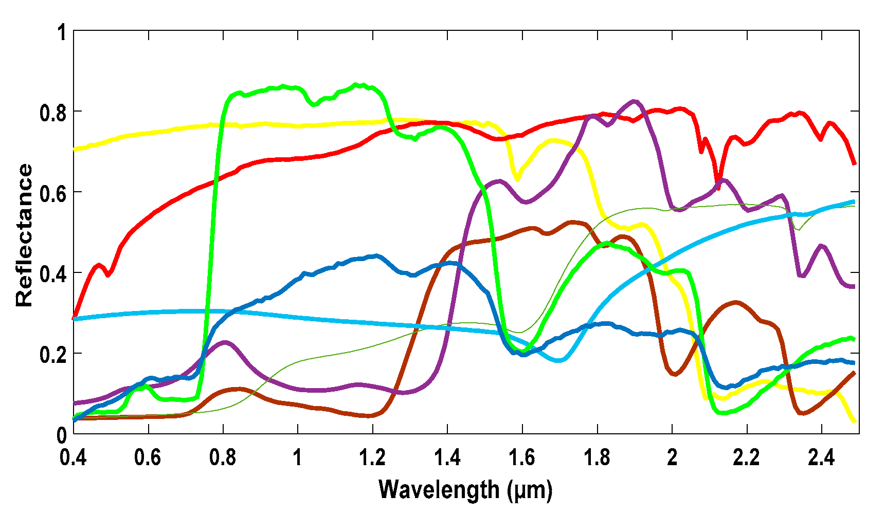
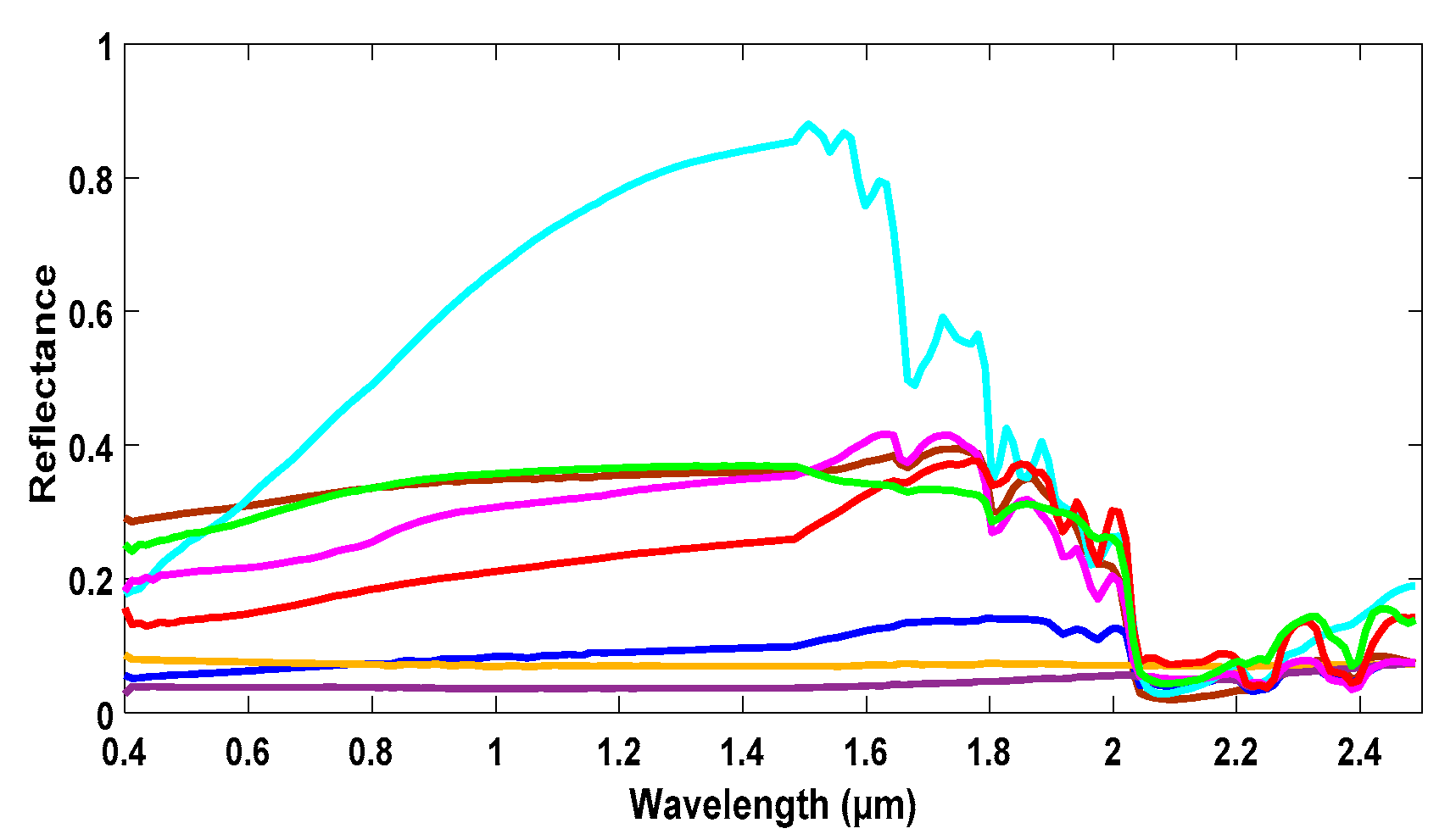
For realistic synthetic hyperspectral data, two sets of eight hyperspectral endmember spectra are selected from spectral libraries, with 184 spectral bands in the 0.4 to 2.5 μm region. The first set contains eight randomly selected spectra (Figure 1) from the spectral library compiled by the United States Geological Survey (USGS) [66]. The second set contains eight spectra (Figure 2) of materials used in urban areas, selected from the spectral library compiled by the Johns Hopkins University (JHU) [67].

The above spectra are used to create two realistic synthetic hyperspectral images. These two 100 × 100 pixel hyperspectral images are generated according to the considered mixing models; the first one is created by considering the bilinear mixing model, whereas the second image is generated by using the LQ model. The considered linear abundance fractions are created from a real classification of land cover, with eight classes, by averaging pixel classification values on a nonoverlapping sliding 4 × 4 pixel window. The second-order abundance fractions are generated from the linear ones by using the Fan model [41]. Besides, it is useful to mention here that the maximum purity of the considered linear abundance fractions does not exceed 0.75 (i.e., without the presence of pure pixels for each endmember), which makes, from the outset, the used synthetic data realistic, with more complex configurations than those with the presence of pure pixels for each endmember.

2.4.2. Real Data

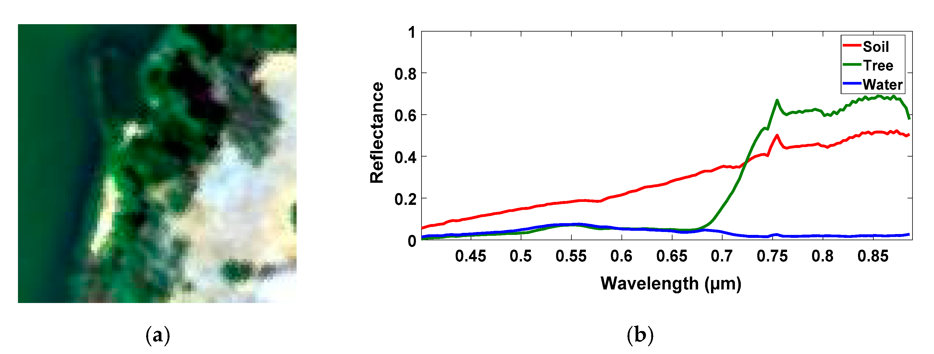
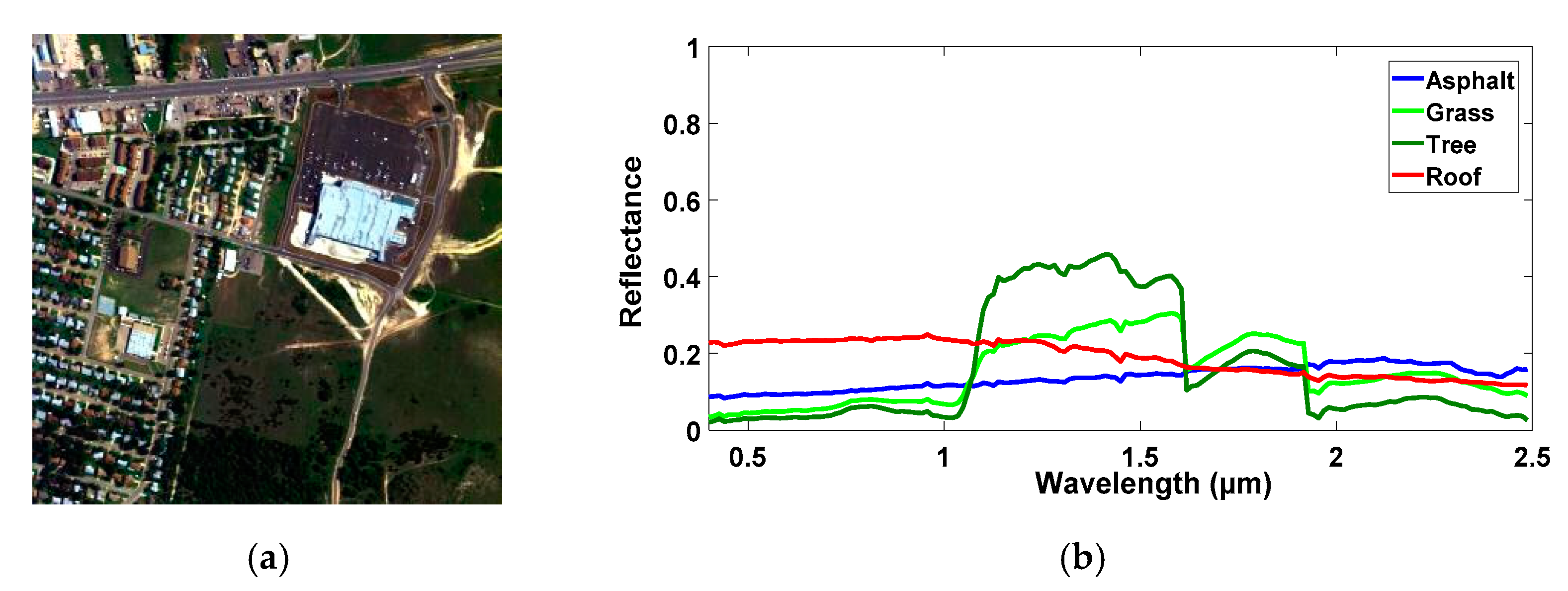
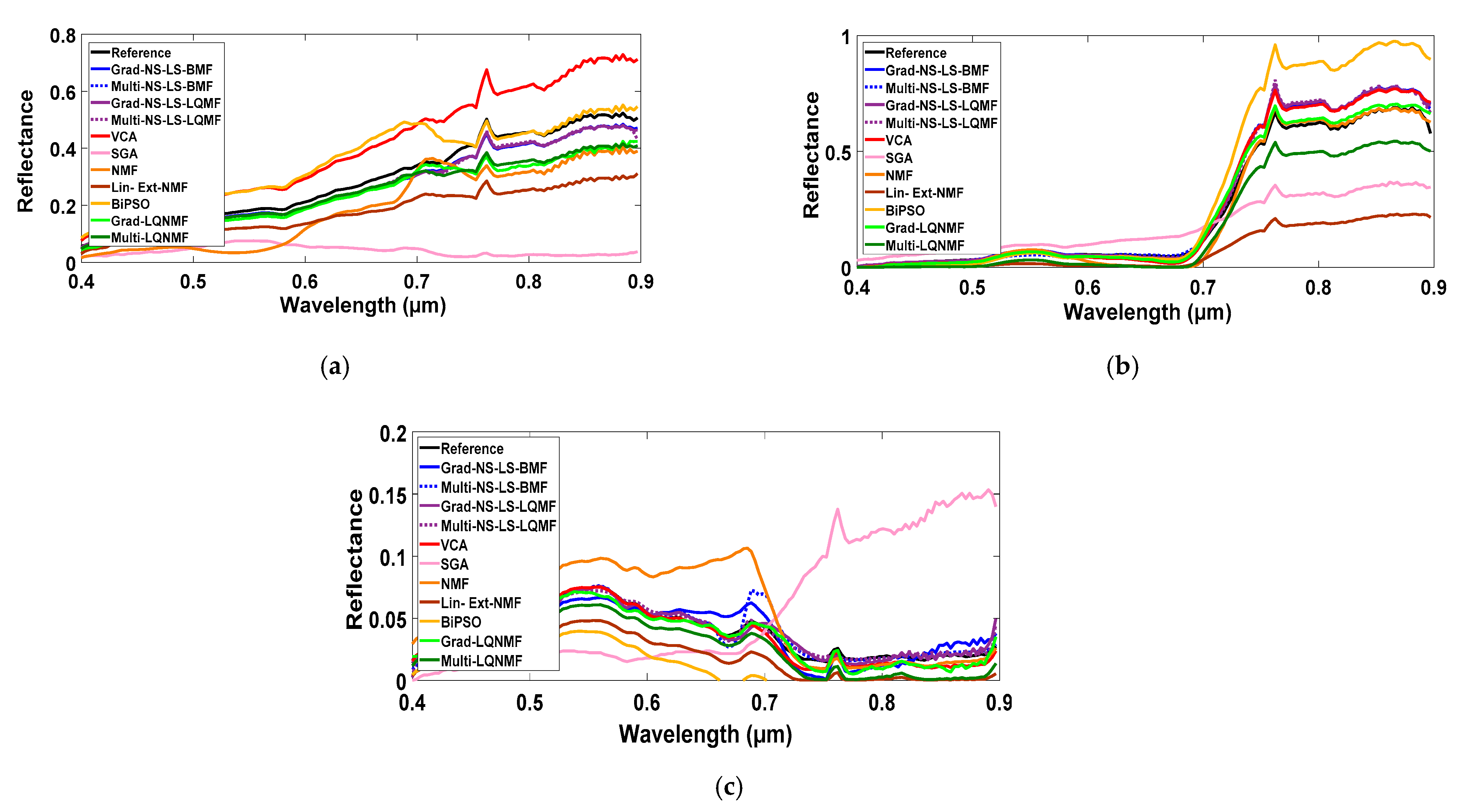
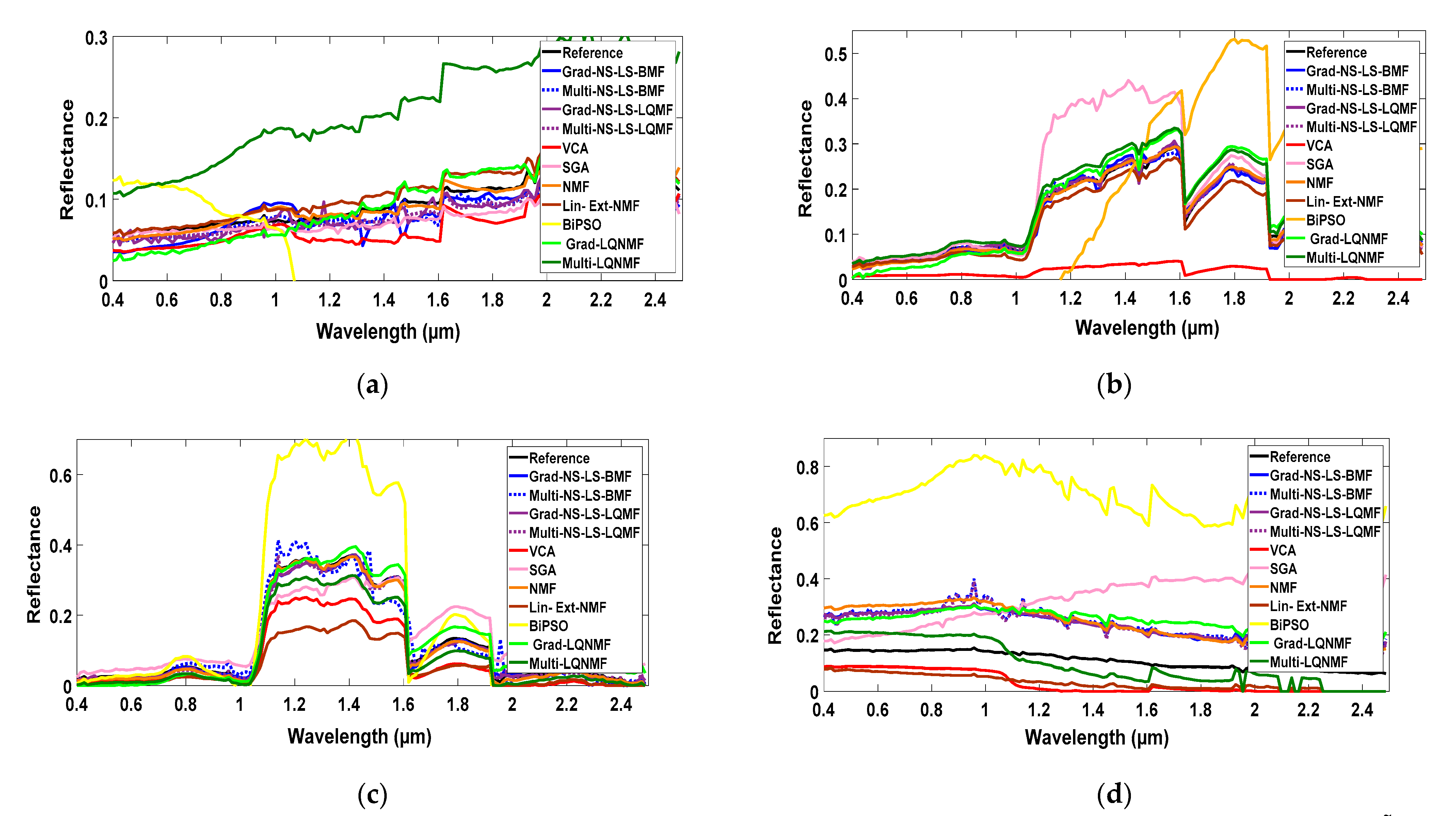
In these investigations, two real hyperspectral images are also considered. The first one consists of the “Samson” data of [68]. This 95 × 95 pixel hyperspectral image (Figure 3a) contains 156 spectral bands ranging from 0.4 to 0.9 μm. Moreover, this first image is provided with the corresponding linear abundance fraction ground-truth, which is used to manually extract, from supposedly pure pixels, three reference endmember spectra (soil, tree, and water: Figure 3b). The second real hyperspectral image consists of the “urban” data of [68]. This image, which is one of the most widely used hyperspectral data sets, was acquired by the HYperspectral Digital Imagery Collection Experiment (HYDICE) sensor over the Copperas Cove, near Fort Hood, Texas, USA. This 307 × 307 pixel hyperspectral image, with 2 m spatial resolution, contains 162 spectral bands (after removing the water absorption bands from the 210 spectral bands of the original data) ranging from 0.4 to 2.5 μm. This image (Figure 4a), which is provided with the corresponding linear abundance fraction ground-truth, mainly contains four pure materials: asphalt, grass, tree, and roof. By considering the provided ground-truth, the reference endmember spectra (Figure 4b) are manually extracted.

3. Results

3.1. Performance Evaluation Criteria

In order to evaluate the performance of the tested methods, the following criteria are considered. The spectral angle mapper (SAM), the spectral normalized mean square error (${\mathrm{NMSE}}_{\mathsf{\lambda }}$), and the spectral information divergence (SID) [69] are used as spectral performance criteria. The spatial normalized mean square error (${\mathrm{NMSE}}_{\mathrm{s}}$) is used as a spatial performance criterion only by considering the linear abundance fractions. A smaller value of these criteria indicates a better endmember spectra or abundance fraction estimation. These criteria read:

$${\mathrm{SAM}}_j=\arccos \left(\frac{{\mathit{s}}_{\mathit{j}}^{\mathrm{T}}{\tilde{\mathit{s}}}_{\mathit{j}}}{\Vert {\mathit{s}}_{\mathit{j}}\Vert \Vert {\tilde{\mathit{s}}}_{\mathit{j}}\Vert }\right)$$

(41)

$${\mathrm{NMSE}}_{\mathsf{\lambda }}{}_j=\frac{\Vert s_j-{\tilde{\mathit{s}}}_{\mathit{j}}\Vert {}_F^2}{\Vert s_j\Vert {}_F^2}$$

(42)

$${\mathrm{SID}}_j=s_j^{\mathrm{T}}\log \left(\frac{s_j}{{\tilde{s}}_j}\right)+{\tilde{s}}_j^{\mathrm{T}}\log \left(\frac{{\tilde{s}}_j}{s_j}\right)$$

(43)

$${\mathrm{NMSE}}_{\mathrm{s}}{}_j=\frac{\Vert a_j-{\tilde{a}}_j\Vert {}_F^2}{\Vert a_j\Vert {}_F^2}$$

(44)

where $s_j$ is the original spectrum of the endmember$j$ and ${\tilde{s}}_j$ is its estimate, $\Vert .\Vert$ denotes the vector norm, $log\left(.\right)$ corresponds to the natural logarithm, $\oslash$ stands for element-wise division, and $a_j$ is the vector composed of the original linear abundance fractions of the endmember $j$ in all image pixels and ${\tilde{a}}_j$ is its estimate.

3.2. Results

The proposed methods, and methods from the literature are applied to the considered realistic synthetic and real hyperspectral data. The considered literature methods belong to two groups. The first one contains linear spectral unmixing methods: the NMF and the Lin-Ext-NMF (linear-extended non-negative matrix factorization) [47] techniques. It should be noted here that, for the NMF method, only the endmember spectra and linear abundance fractions are considered, while, for the Lin-Ext-NMF technique, in addition to the endmember spectra and linear abundance fractions, the pseudo-endmember spectra (resp. second-order abundance fractions) are considered as additional endmember spectra (resp. additional linear abundance fractions). The VCA [29] and the SGA [4,30,31,32] combined with the fully constrained least squares (FCLS) [64] methods, which belong to this first group, are also considered in the conducted tests. The second group contains spectral unmixing methods based on bilinear or linear-quadratic mixing models. These methods are: the BiPSO (bilinear spectral unmixing using particle swarm optimization) technique [65], the Grad-LQNMF (gradient-based linear-quadratic non-negative matrix factorization), and the Multi-LQNMF (multiplicative linear-quadratic non-negative matrix factorization) algorithms [47] (restricted to the bilinear case when the considered mixing model is bilinear).

In all tested iterative algorithms, a maximum of 1000 iterations are considered in the endmember spectra extraction step, as well as in the abundance fraction estimation step. The convergence tolerance threshold, defined in Equation (37), is set to 10⁻⁶. In addition, in order to determine the optimal value of the learning rate $\alpha$ for all tested gradient-based algorithms, many tests are conducted and $\alpha$ is empirically fixed to 10⁻³ for all of these algorithms in the results reported below. It should be remembered here that this empirically optimal choice of the learning rate value constitutes, as mentioned above, the main limitation of these gradient-based methods.

3.2.1. Initialization and Partial Projection Choices

The proposed methods have limitations, as well as all tested NMF-based and the BiPSO literature methods; they are not guaranteed to provide a unique solution, and their convergence points depend on their initialization. Therefore, in order to avoid the random initialization of the considered variables, and as mentioned above, three standard linear techniques are tested, only on the considered realistic synthetic datasets, to select the most suitable one to derive the initial estimated hyperspectral endmember spectra. These standard linear techniques are: the VCA [29] and the SGA [4,30,31,32] techniques, combined with the FCLS [64] algorithm, and the NICA [16] technique. Furthermore, in order to minimize the random effect of these initialization techniques, 10 runs are performed for each considered dataset and for each considered standard linear initialization technique, and the mean values of the used performance evaluation criteria are reported in the following results tables.

Based on the results of

Table 1. Mean values of the considered performance criteria for the synthetic data generated according to the bilinear mixing model and for the tested initialization methods (bold values correspond to best performances).

		SAM (°)	$\mathbf{N}\mathbf{M}\mathbf{S}{\mathbf{E}}_{\mathsf{\lambda }}(\%)$	SID	$\mathbf{N}\mathbf{M}\mathbf{S}{\mathbf{E}}_{\mathbf{s}}(\%)$
With the first set of spectra	VCA+FCLS	9.63	23.39	6.53	55.49
	SGA+FCLS	15.71	32.06	19.97	107.55
	NICA	92.48	140.27	124.59	267.09
With the second set of spectra	VCA+FCLS	10.23	48.41	4.71	49.07
	SGA+FCLS	10.75	42.77	16.19	108.10
	NICA	89.34	316.72	201.96	266.59

and

Table 2. Mean values of the considered performance criteria for the synthetic data generated according to the LQ mixing model and for the tested initialization methods (bold values correspond to best performances).

		SAM (°)	$\mathbf{N}\mathbf{M}\mathbf{S}{\mathbf{E}}_{\mathsf{\lambda }}(\%)$	SID	$\mathbf{N}\mathbf{M}\mathbf{S}{\mathbf{E}}_{\mathbf{s}}(\%)$
With the first set of spectra	VCA+FCLS	6.23	43.68	15.73	32.60
	SGA+FCLS	14.31	60.41	30.30	85.51
	NICA	26.16	68.10	62.67	104.54
With the second set of spectra	VCA+FCLS	7.01	21.28	5.56	61.81
	SGA+FCLS	12.12	59.72	46.62	120.75
	NICA	29.78	96.79	42.19	172.55

, it clearly appears that VCA is the most suitable standard linear initialization technique that can be used in order to derive initial estimated hyperspectral endmember spectra. Thus, this technique is considered to initialize all proposed methods; all tested NMF-based and the BiPSO literature techniques in the tests reported below.

Moreover, for the proposed multiplicative projective methods, as explained above, two partly projected functions (${\left[.\right]}_{\mathrm{pp}1}$ and ${\left[.\right]}_{\mathrm{pp}2}$) are introduced to take advantage of the multiplicative rule Equation (28) and to ensure the non-negativity constraint. In order to choose the most adequate partial projected function to be considered in these proposed methods, experiments are conducted, again only on the described realistic synthetic datasets, by using these multiplicative projective methods, and by only considering the first approach for estimating abundance fractions (i.e., methods called “Multi-NS-LS-BMF/LQMF + constrained ${\tilde{A}}_{opt}$”). From the obtained results (

Table 3. Mean values of the considered performance criteria for the synthetic data generated according to the bilinear mixing model depending on the partly projected function (bold values correspond to best performances).

			SAM (°)	$$\mathbf{N}\mathbf{M}\mathbf{S}{\mathbf{E}}_{\mathsf{\lambda }}(\%)$$	SID	$$\mathbf{N}\mathbf{M}\mathbf{S}{\mathbf{E}}_{\mathbf{s}}(\%)$$
With the first set of spectra	Multi-NS-LS-BMF	${\left[.\right]}_{\mathrm{pp}1}$	7.83	17.64	3.43	90.43
		${\left[.\right]}_{\mathrm{pp}2}$	25.45	100.00	2.56 × 103	86.95
	Multi-NS-LS-LQMF	${\left[.\right]}_{\mathrm{pp}1}$	7.87	17.69	3.44	81.99
		${\left[.\right]}_{\mathrm{pp}2}$	81.02	100.00	4.25 × 103	122.13
With the second set of spectra	Multi-NS-LS-BMF	${\left[.\right]}_{\mathrm{pp}1}$	3.68	15.06	0.87	77.34
		${\left[.\right]}_{\mathrm{pp}2}$	16.49	100.00	1.28 × 103	86.97
	Multi-NS-LS-LQMF	${\left[.\right]}_{\mathrm{pp}1}$	3.63	15.00	0.86	90.69
		${\left[.\right]}_{\mathrm{pp}2}$	88.74	100.00	3.28 × 103	110.56

and

Table 4. Mean values of the considered performance criteria for the synthetic data generated according to the LQ mixing model depending on the partly projected function (bold values correspond to best performances).

			SAM (°)	$\mathbf{N}\mathbf{M}\mathbf{S}{\mathbf{E}}_{\mathsf{\lambda }}(\%)$	SID	$\mathbf{N}\mathbf{M}\mathbf{S}{\mathbf{E}}_{\mathbf{s}}(\%)$
With the first set of spectra	Multi-NS-LS-BMF	${\left[.\right]}_{\mathrm{pp}1}$	5.48	33.83	9.99	58.75
		${\left[.\right]}_{\mathrm{pp}2}$	25.70	100.00	2.56 × 103	86.91
	Multi-NS-LS-LQMF	${\left[.\right]}_{\mathrm{pp}1}$	5.83	34.44	10.15	70.74
		${\left[.\right]}_{\mathrm{pp}2}$	78.21	100.00	6.34 × 103	136.2
With the second set of spectra	Multi-NS-LS-BMF	${\left[.\right]}_{\mathrm{pp}1}$	5.10	13.79	2.62	72.71
		${\left[.\right]}_{\mathrm{pp}2}$	16.76	100.00	1.28 × 103	86.96
	Multi-NS-LS-LQMF	${\left[.\right]}_{\mathrm{pp}1}$	4.81	13.33	2.54	94.72
		${\left[.\right]}_{\mathrm{pp}2}$	82.32	100.00	2.27 × 103	116.65

), it clearly appears that the first partly projected function (noted ${\left[.\right]}_{\mathrm{pp}1}$) is the most adequate one that can be considered in the proposed multiplicative projective methods. Consequently, this function is the one considered hereafter in these proposed methods.

3.2.2. Results on Synthetic Data

Table 5. Mean values of the considered performance criteria for the synthetic data generated according to the bilinear mixing model and with the first set of spectra (bold values correspond to best performances).

	SAM (°)	$\mathbf{N}\mathbf{M}\mathbf{S}{\mathbf{E}}_{\mathsf{\lambda }}(\%)$	SID	$\mathbf{N}\mathbf{M}\mathbf{S}{\mathbf{E}}_{\mathbf{s}}(\%)$
Grd-NS-LS-BMF + constrained ${\tilde{\mathit{A}}}_{opt}$	7.63	17.37	3.36	31.28
Grd-NS-LS-BMF + post-Multi-LQNMF1	7.63	17.37	3.36	35.98
Grd-NS-LS-BMF + post-Multi-LQNMF2	4.17	9.13	1.21	28.00
Multi-NS-LS-BMF + constrained ${\tilde{\mathit{A}}}_{opt}$	7.83	17.64	3.43	90.43
Multi-NS-LS-BMF + post-Multi-LQNMF1	7.83	17.64	3.43	77.30
Multi-NS-LS-BMF + post-Multi-LQNMF2	12.03	29.21	14.59	86.35
Grd-NS-LS-LQMF + constrained ${\tilde{\mathit{A}}}_{opt}$	7.63	17.37	3.36	30.89
Grd-NS-LS-LQMF + post-Multi-LQNMF1	7.63	17.37	3.36	35.57
Grd-NS-LS-LQMF + post-Multi-LQNMF2	4.11	8.92	1.18	27.27
Multi-NS-LS-LQMF + constrained ${\tilde{\mathit{A}}}_{opt}$	7.87	17.69	3.44	81.99
Multi-NS-LS-LQMF + post-Multi-LQNMF1	7.87	17.69	3.44	75.75
Multi-NS-LS-LQMF + post-Multi-LQNMF2	15.40	33.35	21.19	79.58
VCA+FCLS	9.63	23.39	6.53	55.49
SGA+FCLS	15.71	32.06	19.97	107.55
NMF	12.88	32.05	8.90	59.44
Lin-Ext-NMF	12.13	28.45	11.15	59.05
BiPSO	8.59	19.91	5.36	39.76
Grd-LQNMF	8.39	25.44	10.09	67.85
Multi-LQNMF	12.35	27.27	9.96	56.92

,

Table 6. Mean values of the considered performance criteria for the synthetic data generated according to the bilinear mixing model and with the second set of spectra (bold values correspond to best performances).

	SAM (°)	$\mathbf{N}\mathbf{M}\mathbf{S}{\mathbf{E}}_{\mathsf{\lambda }}(\%)$	SID	$\mathbf{N}\mathbf{M}\mathbf{S}{\mathbf{E}}_{\mathbf{s}}(\%)$
Grd-NS-LS-BMF + constrained ${\tilde{\mathit{A}}}_{opt}$	3.55	14.95	0.86	39.60
Grd-NS-LS-BMF + post-Multi-LQNMF1	3.55	14.95	0.86	39.54
Grd-NS-LS-BMF + post-Multi-LQNMF2	2.54	9.88	0.32	38.34
Multi-NS-LS-BMF + constrained ${\tilde{\mathit{A}}}_{opt}$	3.68	15.06	0.87	77.34
Multi-NS-LS-BMF + post-Multi-LQNMF1	3.68	15.06	0.87	68.54
Multi-NS-LS-BMF + post-Multi-LQNMF2	10.03	39.21	6.84	76.15
Grd-NS-LS-LQMF + constrained ${\tilde{\mathit{A}}}_{opt}$	3.55	14.95	0.86	38.40
Grd-NS-LS-LQMF + post-Multi-LQNMF1	3.55	14.95	0.86	38.37
Grd-NS-LS-LQMF + post-Multi-LQNMF2	2.51	9.72	0.31	36.83
Multi-NS-LS-LQMF + constrained ${\tilde{\mathit{A}}}_{opt}$	3.63	15.00	0.86	90.69
Multi-NS-LS-LQMF + post-Multi-LQNMF1	3.63	15.00	0.86	84.43
Multi-NS-LS-LQMF + post-Multi-LQNMF2	11.05	46.80	9.78	92.22
VCA+FCLS	10.23	48.41	4.71	49.07
SGA+FCLS	10.75	42.77	16.19	108.10
NMF	12.49	34.73	3.22	64.40
Lin-Ext-NMF	12.05	32.02	4.78	65.39
BiPSO	6.83	17.14	1.23	42.99
Grd-LQNMF	6.09	17.82	1.07	68.33
Multi-LQNMF	13.48	28.30	3.47	66.38

,

Table 7. Mean values of the considered performance criteria for the synthetic data generated according to the LQ mixing model and with the first set of spectra (bold values correspond to best performances).

	SAM (°)	$\mathbf{N}\mathbf{M}\mathbf{S}{\mathbf{E}}_{\mathsf{\lambda }}(\%)$	SID	$\mathbf{N}\mathbf{M}\mathbf{S}{\mathbf{E}}_{\mathbf{s}}(\%)$
Grd-NS-LS-BMF + constrained ${\tilde{\mathit{A}}}_{opt}$	5.37	33.70	9.93	35.22
Grd-NS-LS-BMF + post-Multi-LQNMF1	5.37	33.70	9.93	33.81
Grd-NS-LS-BMF + post-Multi-LQNMF2	3.99	17.85	4.55	31.86
Multi-NS-LS-BMF + constrained ${\tilde{\mathit{A}}}_{opt}$	5.48	33.83	9.99	58.75
Multi-NS-LS-BMF + post-Multi-LQNMF1	5.48	33.83	9.99	55.80
Multi-NS-LS-BMF + post-Multi-LQNMF2	11.10	30.45	15.86	57.02
Grd-NS-LS-LQMF + constrained ${\tilde{\mathit{A}}}_{opt}$	5.37	33.70	9.93	24.69
Grd-NS-LS-LQMF + post-Multi-LQNMF1	5.37	33.70	9.93	27.43
Grd-NS-LS-LQMF + post-Multi-LQNMF2	3.63	17.74	4.48	23.40
Multi-NS-LS-LQMF + constrained ${\tilde{\mathit{A}}}_{opt}$	5.83	34.44	10.15	70.74
Multi-NS-LS-LQMF + post-Multi-LQNMF1	5.83	34.44	10.15	56.56
Multi-NS-LS-LQMF + post-Multi-LQNMF2	12.01	30.94	20.66	68.07
VCA+FCLS	6.23	43.68	15.73	32.60
SGA+FCLS	14.31	60.41	30.30	85.51
NMF	12.41	32.72	10.69	52.30
Lin-Ext-NMF	12.10	26.73	10.23	51.70
BiPSO	5.30	35.13	10.74	17.25
Grd-LQNMF	15.80	33.75	65.01	60.98
Multi-LQNMF	11.83	25.24	9.03	49.57

and

Table 8. Mean values of the considered performance criteria for the synthetic data generated according to the LQ mixing model and with the second set of spectra (bold values correspond to best performances).

	SAM (°)	$\mathbf{N}\mathbf{M}\mathbf{S}{\mathbf{E}}_{\mathsf{\lambda }}(\%)$	SID	$\mathbf{N}\mathbf{M}\mathbf{S}{\mathbf{E}}_{\mathbf{s}}(\%)$
Grd-NS-LS-BMF + constrained ${\tilde{\mathit{A}}}_{opt}$	4.72	13.21	2.52	33.17
Grd-NS-LS-BMF + post-Multi-LQNMF1	4.72	13.21	2.52	35.18
Grd-NS-LS-BMF + post-Multi-LQNMF2	3.03	8.52	1.10	33.07
Multi-NS-LS-BMF + constrained ${\tilde{\mathit{A}}}_{opt}$	5.10	13.79	2.62	72.71
Multi-NS-LS-BMF + post-Multi-LQNMF1	5.10	13.79	2.62	65.93
Multi-NS-LS-BMF + post-Multi-LQNMF2	9.18	25.00	9.33	75.61
Grd-NS-LS-LQMF + constrained ${\tilde{\mathit{A}}}_{opt}$	4.72	13.21	2.52	30.41
Grd-NS-LS-LQMF + post-Multi-LQNMF1	4.72	13.21	2.52	33.72
Grd-NS-LS-LQMF + post-Multi-LQNMF2	2.99	8.42	1.08	30.35
Multi-NS-LS-LQMF + constrained ${\tilde{\mathit{A}}}_{opt}$	4.81	13.33	2.54	94.72
Multi-NS-LS-LQMF + post-Multi-LQNMF1	4.81	13.33	2.54	88.27
Multi-NS-LS-LQMF + post-Multi-LQNMF2	7.15	19.23	6.04	79.87
VCA+FCLS	7.01	21.28	5.56	61.81
SGA+FCLS	12.12	59.72	46.62	120.75
NMF	10.14	27.79	10.75	46.93
Lin-Ext-NMF	9.44	20.78	10.24	48.79
BiPSO	7.76	20.21	4.62	35.90
Grd-LQNMF	7.60	18.69	8.29	61.12
Multi-LQNMF	10.48	20.41	8.75	45.55

show the mean values of the considered performance criteria obtained for the realistic synthetic data created according to the bilinear and linear-quadratic mixing models (after performing 10 runs for each considered dataset).

Furthermore, in order to study the effect of noise on the performance of the proposed methods, in particular on their endmember spectra extraction step (by only considering the proposed methods that use “constrained${\tilde{A}}_{opt}$”), and as an illustration, white Gaussian noise with different signal-to-noise ratio (SNR) values, ranging from 15 to 45 decibels (dB) with a step of 5 dB, is added to the created synthetic data generated according to the LQ mixing model and with the urban material spectra. This synthetic dataset is chosen because it is the one which represents the most complete configuration, from the point of view of the mixing model, and it is the most realistic one for LQ mixtures since it considers urban material spectra. The next figure (Figure 5) shows the obtained mean values of the considered performance criteria on the tested synthetic data.

From these results, it clearly appears that the considered proposed methods remain, overall, robust to the considered noise (with different SNR values), and also offer, globally, better performances than those provided by the tested approaches from the literature.

3.2.3. Results on Real Data

The test results obtained for the two considered real hyperspectral images are provided in

Table 9. Mean values of the considered performance criteria for the real Samson data (bold values correspond to best performances).

	SAM (°)	$\mathbf{N}\mathbf{M}\mathbf{S}{\mathbf{E}}_{\mathsf{\lambda }}(\%)$	SID	$\mathbf{N}\mathbf{M}\mathbf{S}{\mathbf{E}}_{\mathbf{s}}(\%)$
Grd-NS-LS-BMF + constrained ${\tilde{\mathit{A}}}_{opt}$	4.65	16.05	1.27	31.26
Grd-NS-LS-BMF + post-Multi-LQNMF1	4.65	16.05	1.27	26.01
Grd-NS-LS-BMF + post-Multi-LQNMF2	7.94	25.41	4.01	30.46
Multi-NS-LS-BMF + constrained ${\tilde{\mathit{A}}}_{opt}$	5.41	22.32	1.24	48.10
Multi-NS-LS-BMF + post-Multi-LQNMF1	5.41	22.32	1.24	36.82
Multi-NS-LS-BMF + post-Multi-LQNMF2	14.48	89.43	13.44	53.45
Grd-NS-LS-LQMF + constrained ${\tilde{\mathit{A}}}_{opt}$	3.71	14.24	0.91	61.62
Grd-NS-LS-LQMF + post-Multi-LQNMF1	3.71	14.24	0.91	46.78
Grd-NS-LS-LQMF + post-Multi-LQNMF2	9.33	36.65	6.98	72.22
Multi-NS-LS-LQMF + constrained ${\tilde{\mathit{A}}}_{opt}$	2.98	12.77	0.83	53.50
Multi-NS-LS-LQMF + post-Multi-LQNMF1	2.98	12.77	0.83	43.41
Multi-NS-LS-LQMF + post-Multi-LQNMF2	10.21	42.49	7.88	63.41
VCA+FCLS	3.46	16.77	2.01	36.47
SGA+FCLS	23.16	72.60	5.40	166.49
NMF	11.79	38.23	6.43	86.31
Lin-Ext-NMF	7.43	51.83	14.32	23.74
BiPSO	28.52	58.57	4.25	57.56
Grd-LQNMF	5.69	18.19	1.99	25.02
Multi-LQNMF	5.76	20.80	3.04	28.41

and

Table 10. Mean values of the considered performance criteria for the real urban data (bold values correspond to best performances).

	SAM (°)	$\mathbf{N}\mathbf{M}\mathbf{S}{\mathbf{E}}_{\mathsf{\lambda }}(\%)$	SID	$\mathbf{N}\mathbf{M}\mathbf{S}{\mathbf{E}}_{\mathbf{s}}(\%)$
Grd-NS-LS-BMF + constrained ${\tilde{\mathit{A}}}_{opt}$	17.73	67.00	14.08	50.01
Grd-NS-LS-BMF + post-Multi-LQNMF1	17.73	67.00	14.08	40.21
Grd-NS-LS-BMF + post-Multi-LQNMF2	15.42	53.73	14.24	34.27
Multi-NS-LS-BMF + constrained ${\tilde{\mathit{A}}}_{opt}$	7.31	28.11	4.21	39.68
Multi-NS-LS-BMF + post-Multi-LQNMF1	7.31	28.11	4.21	31.42
Multi-NS-LS-BMF + post-Multi-LQNMF2	15.35	45.43	11.87	22.93
Grd-NS-LS-LQMF + constrained ${\tilde{\mathit{A}}}_{opt}$	18.06	65.81	12.66	58.84
Grd-NS-LS-LQMF + post-Multi-LQNMF1	18.06	65.81	12.66	44.88
Grd-NS-LS-LQMF + post-Multi-LQNMF2	19.83	64.12	24.12	56.04
Multi-NS-LS-LQMF + constrained ${\tilde{\mathit{A}}}_{opt}$	6.34	24.43	2.00	76.05
Multi-NS-LS-LQMF + post-Multi-LQNMF1	6.34	24.43	2.00	40.02
Multi-NS-LS-LQMF + post-Multi-LQNMF2	14.90	50.94	16.41	63.38
VCA+FCLS	26.38	82.53	42.28	81.98
SGA+FCLS	17.35	67.87	20.73	121.97
NMF	11.79	36.63	4.56	43.03
Lin-Ext-NMF	14.95	51.14	18.43	46.63
BiPSO	49.34	171.24	42.45	59.46
Grd-LQNMF	32.75	85.79	91.61	63.46
Multi-LQNMF	10.96	46.78	9.12	30.40

(after performing 10 runs for each considered dataset).

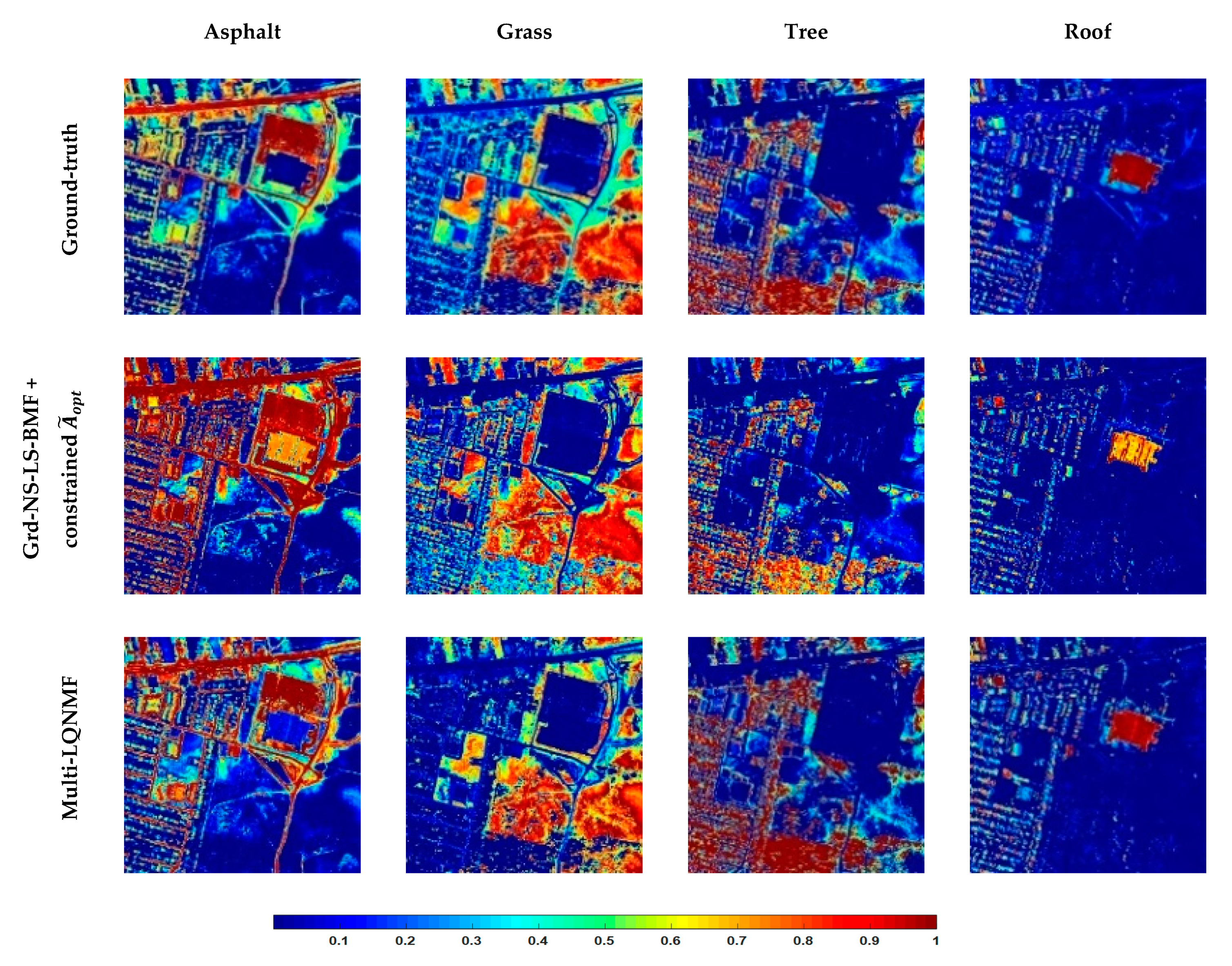
As an illustration, Figure 6 and Figure 7 show, for real data, the reference endmember spectra (ground truth) and their estimates derived by the proposed four methods that use “constrained${\tilde{A}}_{opt}$” and by the considered methods from the literature. Figure 8 and Figure 9 then show, also as an illustration, the ground-truth linear abundance fraction maps and their estimates provided by the proposed Grd-NS-LS-BMF + constrained ${\tilde{A}}_{opt}$ method, and also those provided by the tested Multi-LQNMF literature one.

4. Discussion

For the synthetic data generated according to the bilinear mixing model, Table 5 and Table 6 first yield the following conclusions with respect to the estimated endmember spectra. Among the proposed methods, the four methods that use “constrained${\tilde{A}}_{opt}$” (i.e., “Grd-NS-LS-BMF + constrained${\tilde{A}}_{opt}$” and so on), and hence the four methods that use “post-Multi-LQNMF1” (i.e., “Grd-NS-LS-BMF + post-Multi-LQNMF1” and so on), yield a relatively similar performance. Indeed, for the spectra used in Table 5, the SAM values of these methods are between 7.63 and 7.87°, their ${\mathrm{NMSE}}_{\mathsf{\lambda }}$ values are between 17.37 and 17.69%, and their SID values are between 3.36 and 3.44. For the spectra used in Table 6, their SAM values are between 3.55 and 3.68°, their ${\mathrm{NMSE}}_{\mathsf{\lambda }}$ values are between 14.95 and 15.06%, and their SID values are between 0.86 and 0.87. These methods are, therefore, more attractive than the four methods that use “post-Multi-LQNMF2” (i.e., “Grd-NS-LS-BMF + post-Multi-LQNMF2” and so on), since the latter methods yield significantly wider ranges for the considered performance criteria values and are thus “less predictable”. Indeed, for the spectra used in Table 5, their SAM values are between 4.11 and 15.40°, their ${\mathrm{NMSE}}_{\mathsf{\lambda }}$ values are between 8.92 and 33.35%, and their SID values are between 1.18 and 21.19. For the spectra used in Table 6, their SAM values are between 2.51 and 11.05°, their ${\mathrm{NMSE}}_{\mathsf{\lambda }}$ values are between 9.72 and 46.80%, and their SID values are between 0.31 and 9.78. Similarly, the eight proposed methods that use “constrained${\tilde{A}}_{opt}$” or “post-Multi-LQNMF1” are more attractive than the methods from the literature, since the considered performance criteria values achieved by the latter methods are higher and cover a wide range. Indeed, for these literature methods, in Table 5, the SAM values are between 8.39 and 15.71°, the ${\mathrm{NMSE}}_{\mathsf{\lambda }}$ values are between 19.91 and 32.06%, and the SID values are between 5.36 and 19.97. In Table 6, the SAM values are between 6.09 and 13.48°, the ${\mathrm{NMSE}}_{\mathsf{\lambda }}$ values are between 17.14 and 48.41%, and the SID values are between 1.07 and 16.19.

Considering, in addition, the accuracy of abundance estimation and focusing on the above-defined eight preferred proposed methods, the subset of four gradient-based methods yields much lower ${\mathrm{NMSE}}_{\mathrm{s}}$ values (from 30.89 to 35.98% in Table 5, and from 38.37 to 39.60% in Table 6) than the four multiplicative methods (${\mathrm{NMSE}}_{\mathrm{s}}$ values from 75.75 to 90.43% in Table 5, and from 68.54 to 90.69% in Table 6). Although the errors of these gradient-based methods are non-negligible, they are much better (i.e., lower, and with lower spread) than those of the methods from the literature, which yield NMSES values ranging from 39.76 to 107.55% in Table 5, and from 42.99 to 108.10% in Table 6.

For the synthetic data generated according to the LQ mixing model, Table 7 and Table 8 yield the same general conclusions as above, based on the following values. The eight proposed methods that use “constrained ${\tilde{A}}_{opt}$” or “post-Multi-LQNMF1” result in SAM values ranging from 5.37 to 5.83° in Table 7, and from 4.72 to 5.10° in Table 8. Moreover, these methods result in ${\mathrm{NMSE}}_{\mathsf{\lambda }}$ values ranging from 33.70 to 34.44% in Table 7, and from 13.21 to 13.79% in Table 8. Furthermore, these methods result in SID values ranging from 9.93 to 10.15 in Table 7, and from 2.52 to 2.62 in Table 8. For the four methods that use “post-Multi-LQNMF2”, the SAM ranges from 3.63 to 12.01° in Table 7, and from 2.99 to 9.18° in Table 8. The ${\mathrm{NMSE}}_{\mathsf{\lambda }}$ ranges from 17.74 to 30.94% in Table 7, and from 8.42 to 25.00% in Table 8. Moreover, the SID ranges from 4.48 to 20.66 in Table 7, and from 1.08 to 9.33 in Table 8. For the methods from the literature, the SAM ranges from 5.30 to 15.80° in Table 7, and from 7.01 to 12.12° in Table 8. Their ${\mathrm{NMSE}}_{\mathsf{\lambda }}$ ranges from 25.24 to 60.41% in Table 7, and from 18.69 to 59.72% in Table 8. Finally, their SID ranges from 9.03 to 65.01 in Table 7, and from 4.62 to 46.62 in Table 8. Similarly, the ranges of ${\mathrm{NMSE}}_{\mathrm{s}}$ values respectively for Table 7 and Table 8 are (24.69%, 35.22%) and (30.41%, 35.18%) for the four selected gradient-based methods, (55.80%, 70.74%]) and (65.93%, 94.72%) for the four selected multiplicative methods, and (32.60%, 85.51%) and (45.55%, 120.75%) for the methods from the literature, except BiPSO. The BiPSO method here yields attractive ${\mathrm{NMSE}}_{\mathrm{s}}$ values (17.25% and 35.90%, respectively, in Table 7 and Table 8), but it is eventually not of interest as compared with the best methods proposed in this paper, because it yields very poor performance for real data, as shown further in this paper.

For the first tested real hyperspectral image, Table 9 yields the following results. The eight proposed methods that use “constrained${\tilde{A}}_{opt}$” or “post-Multi-LQNMF1” result in SAM values between 2.98 and 5.41°, ${\mathrm{NMSE}}_{\mathsf{\lambda }}$ values between 12.77 and 22.32%, and the SID ranges from 0.83 to 1.27. For the four methods that use “post-Multi-LQNMF2”, the SAM ranges from 7.94 to 14.48°, the ${\mathrm{NMSE}}_{\mathsf{\lambda }}$ ranges from 25.41 to 89.43%, and SID values are between 4.01 and 13.44. Besides, the tested literature methods provide SAM values between 3.46 and 28.52°, ${\mathrm{NMSE}}_{\mathsf{\lambda }}$ values between 16.77 and 72.60%, and SID values ranging from 1.99 to 14.32. Similarly, the ranges of ${\mathrm{NMSE}}_{\mathrm{s}}$ values are (26.01%, 61.62%) for the four selected gradient-based methods, (36.82%, 53.50%) for the four selected multiplicative methods, (36.47%, 166.49%) for the methods from the literature, except Lin-Ext-NMF, Grd-LQNMF and Multi-LQNMF. The latter three methods here yield rather good ${\mathrm{NMSE}}_{\mathrm{s}}$ values (between 23.74 and 28.41%), but they are globally not of interest as compared with the best methods proposed in this work, because they yield very poor performance for synthetic data (see Table 5, Table 6, Table 7 and Table 8) and they are, therefore, not predictable enough. This first real image consequently yields the same global remarks as the considered synthetic data, even though some of these trends are less pronounced here. Especially, the considered performance criteria values obtained with the eight preferred methods, among those proposed in this work, have larger ranges here than for the considered synthetic data.

The second tested real hyperspectral image yields the following values (see Table 10). For the eight proposed methods that use “constrained${\tilde{A}}_{opt}$” or “post-Multi-LQNMF1”, the SAM values are between 6.34 and 18.06°, the ${\mathrm{NMSE}}_{\mathsf{\lambda }}$ values are between 24.43 and 67.00%, and the SID ranges from 2.00 and 14.08. For the four methods that use “post-Multi-LQNMF2”, the SAM criterion ranges from 14.90 to 19.83°, the ${\mathrm{NMSE}}_{\mathsf{\lambda }}$ ranges from 45.43 to 64.12%, and SID values are between 11.87 and 24.12. For the methods from the literature, the SAM ranges from 10.96 to 49.34°, the ${\mathrm{NMSE}}_{\mathsf{\lambda }}$ ranges from 36.63 to 171.24%, and the SID ranges from 4.56 to 91.61, the worst performances being, globally, obtained with the BiPSO method. Similarly, the ranges of ${\mathrm{NMSE}}_{\mathrm{s}}$ values are (40.21%, 58.84%) for the four selected gradient-based methods, (31.42%, 76.05%) for the four selected multiplicative methods, and (43.03%, 121.97%) for the methods from the literature, except Multi-LQNMF. For this second tested real image, the Multi-LQNMF method yields a rather good ${\mathrm{NMSE}}_{\mathrm{s}}$ value (30.40%), but it is globally not of interest when compared with the best methods proposed in this paper, because it yields very poor performance for synthetic data, as shown above (Table 5, Table 6, Table 7 and Table 8). This second tested real image, therefore, also tends to yield the same global conclusions as with synthetic data, although some of these trends here are not very significant. In particular, the used performance criteria values obtained with the eight preferred methods, among those proposed in this paper, exhibit larger spreads than for synthetic data.

Figure 6 and Figure 7 show that the mentioned proposed methods, unlike the tested literature approaches, correctly extract most of endmember spectra, with estimates fairly close to the reference ones. From Figure 8 and Figure 9, it also clearly appears that the mentioned proposed method correctly estimates the considered abundance fraction maps.

All of the above results clearly show that the proposed gradient-based methods globally provide better performances than those resulting from the proposed multiplicative projective ones, and also from those obtained by the tested literature approaches. However, once again, it should be remembered that these gradient-based methods only provide such results after an optimal choice of their learning rates, which are tedious to obtain, since it is necessary to perform several tests to find these optimal parameter values. In contrast, the proposed multiplicative projective methods are free from this constraint, and they provide satisfactory results that are, moreover, globally better than those of the tested literature methods. They are, therefore, an attractive alternative to gradient-based methods when automated operation is an important feature.

The proposed methods are very easy to implement and their update rules contain only direct and simple scalar/matrix operations. These operations make the algorithmic complexity of the proposed methods very limited. Besides, the run time of the core of the proposed methods depends on the input image size, the number of endmembers in the observed scene, the maximum number of iterations, and the stopping criterion Equation (37); based on the above description of tests by considering, as an illustration, the used synthetic data, the run time of the proposed methods (by using an Intel(R) Core(TM) i7 processor running at 2.40 GHz and a memory capacity of 8 GB) is about, for each run, 10 (respectively 40) seconds for the gradient-based (respectively multiplicative) methods that use “constrained ${\tilde{A}}_{opt}$”, and 20 (respectively 50) seconds for the gradient-based (respectively multiplicative) methods that use “post-Multi-LQNMF”.

5. Conclusions

In this paper, various unsupervised hyperspectral unmixing approaches, based on extensions of matrix factorization with non-negativity constraints and targeted at bilinear or linear-quadratic mixing models, are introduced. For each of these models, firstly, two approaches respectively based on projected gradient descent and multiplicative algorithms are proposed for extracting hyperspectral endmember spectra. The reduction of the number of variables manipulated in these algorithms constitutes the main originality of the proposed approaches. Moreover, three methods are then proposed to extend the above algorithms so as to estimate the proportions, i.e., abundance fractions, of the endmembers and to possibly refine the endmember spectra estimates. This eventually results in 12 versions of the proposed overall unmixing methods.

Experiments, based on realistic synthetic hyperspectral data, generated according to the two considered bilinear and linear-quadratic mixing models, and also on two real hyperspectral images, were conducted with the above 12 proposed methods, and with seven methods from the literature. The efficiency of all these methods was evaluated with established performance criteria. The obtained results show that the preferred proposed methods yield very satisfactory results, especially for hyperspectral endmember spectra extraction. Moreover, the preferred proposed algorithms significantly outperform the tested methods from the literature.

An interesting extension of this work may consist of using the proposed approaches in the unmixing-based hypersharpening process. Indeed, the proposed approaches may be used to extract spectral information from a high spectral resolution observable remote sensing image and spatial information from a high spatial resolution one that covers the same considered area. Then, the extracted high-resolution information will be merged, according to the considered bilinear or linear-quadratic mixing model, to form an unobservable remote sensing image with high spectral and spatial resolutions.

References

1. Weber, C.; Aguejdad, R.; Briottet, X.; Avala, J.; Fabre, S.; Demuynck, J.; Zenou, E.; Deville, Y.; Karoui, M.S.; Benhalouche, F.Z.; et al. Hyperspectral imagery for environmental urban planning. In Proceedings of the IGARSS 2018—2018 IEEE International Geoscience and Remote Sensing Symposium, Valencia, Spain, 22–27 July 2018; pp. 1628–1631. [Google Scholar]
2. Brabant, C.; Alvarez-Vanhard, E.; Laribi, A.; Morin, G.; Thanh Nguyen, K.; Thomas, A.; Houet, T. Comparison of hyperspectral techniques for urban tree diversity classification. Remote Sens. 2019, 11, 1269. [Google Scholar] [CrossRef] [Green Version]
3. Karoui, M.S.; Benhalouche, F.Z.; Deville, Y.; Djerriri, K.; Briottet, X.; Houet, T.; Le Bris, A.; Weber, C. Partial linear nmf-based unmixing methods for detection and area estimation of photovoltaic panels in urban hyperspectral remote sensing data. Remote Sens. 2019, 11, 2164. [Google Scholar] [CrossRef] [Green Version]
4. Chang, C.-I. Hyperspectral Data Processing: Algorithm Design and Analysis; John Wiley&Sons: Hoboken, NJ, USA, 2013. [Google Scholar]
5. Keshava, N.; Mustard, J.F. Spectral unmixing. IEEE Signal Process. Mag. 2002, 19, 44–57. [Google Scholar] [CrossRef]
6. Chang, C.-I.; Chiang, S.-S.; Smith, J.; Ginsberg, I. Linear spectral random mixture analysis for hyperspectral imagery. IEEE Trans. Geosci. Remote Sens. 2002, 40, 375–392. [Google Scholar] [CrossRef]
7. Bioucas-Dias, J.M.; Plaza, A.; Dobigeon, N.; Parente, M.; Du, Q.; Gader, P.; Chanussot, J. Hyperspectral unmixing overview: Geometrical, statistical, and sparse regression-based approaches. IEEE J. Sel. Top. Appl. Earth Obs. Remote Sens. 2012, 5, 354–379. [Google Scholar] [CrossRef] [Green Version]
8. Comon, P.; Jutten, C. Handbook of Blind Source Separation: Independent Component Analysis and Applications, 1st ed.; Academic Press: Oxford, UK, 2010; ISBN 978-0-12-374726-6. [Google Scholar]
9. Deville, Y. Blind source separation and blind mixture identification methods. In Wiley Encyclopedia of Electrical and Electronics Engineering; John Wiley & Sons, Inc.: Hoboken, NJ, USA, 2016; pp. 1–33. ISBN 978-0-471-34608-1. [Google Scholar]
10. Wang, J.; Chang, C.-I. Applications of independent component analysis in endmember extraction and abundance quantification for hyperspectral imagery. IEEE Trans. Geosci. Remote Sens. 2006, 44, 2601–2616. [Google Scholar] [CrossRef]
11. Moussaoui, S.; Hauksdóttir, H.; Schmidt, F.; Jutten, C.; Chanussot, J.; Brie, D.; Douté, S.; Benediktsson, J.A. On the decomposition of mars hyperspectral data by ica and bayesian positive source separation. Neurocomputing 2008, 71, 2194–2208. [Google Scholar] [CrossRef] [Green Version]
12. Xia, W.; Liu, X.; Wang, B.; Zhang, L. Independent component analysis for blind unmixing of hyperspectral imagery with additional constraints. IEEE Trans. Geosci. Remote Sens. 2011, 49, 2165–2179. [Google Scholar] [CrossRef]
13. Plumbley, M.D. Conditions for nonnegative independent component analysis. IEEE Signal Process. Lett. 2002, 9, 177–180. [Google Scholar] [CrossRef] [Green Version]
14. Plumbley, M.D. Algorithms for nonnegative independent component analysis. IEEE Trans. Neural Netw. 2003, 14, 534–543. [Google Scholar] [CrossRef]
15. Plumbley, M.D. Optimization using fourier expansion over a geodesic for non-negative ICA. In Independent Component Analysis and Blind Signal Separation; Puntonet, C.G., Prieto, A., Eds.; Lecture Notes in Computer Science; Springer: Berlin/Heidelberg, Germany, 2004; Volume 3195, pp. 49–56. ISBN 978-3-540-23056-4. [Google Scholar]
16. Ouedraogo, W.S.B.; Souloumiac, A.; Jutten, C. Non-negative independent component analysis algorithm based on 2D givens rotations and a newton optimization. In Latent Variable Analysis and Signal Separation; Lecture Notes in Computer Science; Springer: Berlin/Heidelberg, Germany, 2010; Volume 6365, pp. 522–529. ISBN 978-3-642-15994-7. [Google Scholar]
17. Iordache, M.-D.; Bioucas-Dias, J.M.; Plaza, A. Sparse unmixing of hyperspectral data. IEEE Trans. Geosci. Remote Sens. 2011, 49, 2014–2039. [Google Scholar] [CrossRef] [Green Version]
18. Karoui, M.S.; Deville, Y.; Hosseini, S.; Ouamri, A. Blind spatial unmixing of multispectral images: New methods combining sparse component analysis, clustering and non-negativity constraints. Pattern Recognit. 2012, 45, 4263–4278. [Google Scholar] [CrossRef]
19. Karoui, M.S.; Deville, Y.; Hosseini, S.; Ouamri, A. Blind unmixing of hyperspectral data with some pure pixels: Spatial variance-based methods exploiting sparsity and non-negativity properties. In Signal Processing: New Research; Naik, G.R., Ed.; Nova Science Publishers: New York, NY, USA, 2013; pp. 161–182. ISBN 978-1-62808-141-1. [Google Scholar]
20. Zhang, S.; Li, J.; Li, H.-C.; Deng, C.; Plaza, A. Spectral–spatial weighted sparse regression for hyperspectral image unmixing. IEEE Trans. Geosci. Remote Sens. 2018, 56, 3265–3276. [Google Scholar] [CrossRef]
21. Lee, D.D.; Seung, H.S. Learning the parts of objects by non-negative matrix factorization. Nature 1999, 401, 788–791. [Google Scholar] [CrossRef]
22. Lee, D.D.; Seung, H.S. Algorithms for non-negative matrix factorization. Adv. Neural Inf. Process. Syst. 2001, 13, 556–562. [Google Scholar]
23. Cichocki, A.; Zdunek, R.; Phan, A.H.; Amari, S. Nonnegative Matrix and Tensor Factorizations: Applications to Exploratory Multi-Way Data Analysis and Blind Source Separation; John Wiley and Sons: Hoboken, NJ, USA, 2009. [Google Scholar]
24. Lu, X.; Wu, H.; Yuan, Y.; Yan, P.; Li, X. Manifold regularized sparse NMF for hyperspectral unmixing. IEEE Trans. Geosci. Remote Sens. 2013, 51, 2815–2826. [Google Scholar] [CrossRef]
25. Tsinos, C.G.; Rontogiannis, A.A.; Berberidis, K. Distributed blind hyperspectral unmixing via joint sparsity and low-rank constrained non-negative matrix factorization. IEEE Trans. Comput. Imaging 2017, 3, 160–174. [Google Scholar] [CrossRef]
26. Ren, H.; Chang, C. Automatic spectral target recognition in hyperspectral imagery. IEEE Trans. Aerosp. Electron. Syst. 2003, 39, 1232–1249. [Google Scholar] [CrossRef] [Green Version]
27. Chang, C.-I.; Plaza, A. A fast iterative algorithm for implementation of pixel purity index. IEEE Geosci. Remote Sens. Lett. 2006, 3, 63–67. [Google Scholar] [CrossRef]
28. Winter, M.E. N-FINDR: An algorithm for fast autonomous spectral end-member determination in hyperspectral data. In Proceedings of the SPIE’s International Symposium on Optical Science, Engineering, and Instrumentation, Denver, CO, USA, 18–23 July 1999; Descour, M.R., Shen, S.S., Eds.; International Society for Optics and Photonics: Bellingham, WA, USA; Volume 3753, pp. 266–275. [Google Scholar]
29. Nascimento, J.M.P.; Dias, J.M.B. Vertex component analysis: A fast algorithm to unmix hyperspectral data. IEEE Trans. Geosci. Remote Sens. 2005, 43, 898–910. [Google Scholar] [CrossRef] [Green Version]
30. Chang, C.-I.; Wu, C.-C.; Liu, W.; Ouyang, Y.-C. A New growing method for simplex-based endmember extraction algorithm. IEEE Trans. Geosci. Remote Sens. 2006, 44, 2804–2819. [Google Scholar] [CrossRef]
31. Chang, C.-I.; Wu, C.-C.; Lo, C.-S.; Chang, M.-L. Real-time simplex growing algorithms for hyperspectral endmember extraction. IEEE Trans. Geosci. Remote Sens. 2010, 48, 1834–1850. [Google Scholar] [CrossRef]
32. Chang, C.-I.; Chen, S.-Y.; Li, H.-C.; Chen, H.-M.; Wen, C.-H. Comparative study and analysis among ATGP, VCA, and SGA for finding endmembers in hyperspectral imagery. IEEE J. Sel. Top. Appl. Earth Obs. Remote Sens. 2016, 9, 4280–4306. [Google Scholar] [CrossRef]
33. Miao, L.; Qi, H. Endmember extraction from highly mixed data using minimum volume constrained nonnegative matrix factorization. IEEE Trans. Geosci. Remote Sens. 2007, 45, 765–777. [Google Scholar] [CrossRef]
34. Li, J.; Bioucas-Dias, J.M. Minimum volume simplex analysis: A fast algorithm to unmix hyperspectral data. In Proceedings of the IGARSS 2008—2008 IEEE International Geoscience and Remote Sensing Symposium, Boston, MA, USA, 8–11 July 2008; IEEE: Boston, MA, USA. [Google Scholar]
35. Bioucas-Dias, J.M. A variable splitting augmented lagrangian approach to linear spectral unmixing. In Proceedings of the 2009 First Workshop on Hyperspectral Image and Signal Processing: Evolution in Remote Sensing, Grenoble, France, 26–28 August 2009; pp. 1–4. [Google Scholar]
36. Dobigeon, N.; Tourneret, J.-Y.; Richard, C.; Bermudez, J.C.M.; McLaughlin, S.; Hero, A.O. Nonlinear unmixing of hyperspectral images: Models and algorithms. IEEE Signal Process. Mag. 2014, 31, 82–94. [Google Scholar] [CrossRef] [Green Version]
37. Heylen, R.; Parente, M.; Gader, P. A review of nonlinear hyperspectral unmixing methods. IEEE J. Sel. Top. Appl. Earth Obs. Remote Sens. 2014, 7, 1844–1868. [Google Scholar] [CrossRef]
38. Heylen, R.; Scheunders, P. A multilinear mixing model for nonlinear spectral unmixing. IEEE Trans. Geosci. Remote Sens. 2016, 54, 240–251. [Google Scholar] [CrossRef]
39. Meganem, I.; Deliot, P.; Briottet, X.; Deville, Y.; Hosseini, S. Linear–quadratic mixing model for reflectances in urban environments. IEEE Trans. Geosci. Remote Sens. 2014, 52, 544–558. [Google Scholar] [CrossRef]
40. Nascimento, J.M.P.; Bioucas-Dias, J.M. Nonlinear mixture model for hyperspectral unmixing. In Proceedings of the SPIE 7477, Image and Signal Processing for Remote Sensing, Berlin, Germany, 31 August–3 September 2009; Volume 15. [Google Scholar]
41. Fan, W.; Hu, B.; Miller, J.; Li, M. Comparative study between a new nonlinear model and common linear model for analysing laboratory simulated-forest hyperspectral data. Int. J. Remote Sens. 2009, 30, 2951–2962. [Google Scholar] [CrossRef]
42. Halimi, A.; Altmann, Y.; Dobigeon, N.; Tourneret, J.-Y. Nonlinear unmixing of hyperspectral images using a generalized bilinear model. IEEE Trans. Geosci. Remote Sens. 2011, 49, 4153–4162. [Google Scholar] [CrossRef] [Green Version]
43. Altmann, Y.; Halimi, A.; Dobigeon, N.; Tourneret, J.-Y. Supervised nonlinear spectral unmixing using a postnonlinear mixing model for hyperspectral imagery. IEEE Trans. Image Process. 2012, 21, 3017–3025. [Google Scholar] [CrossRef] [Green Version]
44. Altmann, Y.; Dobigeon, N.; McLaughlin, S.; Tourneret, J.-Y. Nonlinear spectral unmixing of hyperspectral images using gaussian processes. IEEE Trans. Signal Process. 2013, 61, 2442–2453. [Google Scholar] [CrossRef] [Green Version]
45. Altmann, Y.; Dobigeon, N.; Tourneret, J.-Y. Unsupervised post-nonlinear unmixing of hyperspectral images using a hamiltonian monte carlo algorithm. IEEE Trans. Image Process. 2014, 23, 2663–2675. [Google Scholar] [CrossRef] [PubMed] [Green Version]
46. Eches, O.; Guillaume, M. A bilinear–bilinear nonnegative matrix factorization method for hyperspectral unmixing. IEEE Geosci. Remote Sens. Lett. 2014, 11, 778–782. [Google Scholar] [CrossRef]
47. Meganem, I.; Deville, Y.; Hosseini, S.; Deliot, P.; Briottet, X. Linear-quadratic blind source separation using NMF to unmix urban hyperspectral images. IEEE Trans. Signal Process. 2014, 62, 1822–1833. [Google Scholar] [CrossRef]
48. Wei, Q.; Chen, M.; Tourneret, J.-Y.; Godsill, S. Unsupervised nonlinear spectral unmixing based on a multilinear mixing model. IEEE Trans. Geosci. Remote Sens. 2017, 55, 4534–4544. [Google Scholar] [CrossRef] [Green Version]
49. Pu, H.; Chen, Z.; Wang, B.; Xia, W. Constrained least squares algorithms for nonlinear unmixing of hyperspectral imagery. IEEE Trans. Geosci. Remote Sens. 2015, 53, 1287–1303. [Google Scholar] [CrossRef]
50. Broadwater, J.; Chellappa, R.; Banerjee, A.; Burlina, P. Kernel fully constrained least squares abundance estimates. In Proceedings of the IGARSS 2007—2007 IEEE International Geoscience and Remote Sensing Symposium, Barcelona, Spain, 23–27 July 2007; pp. 4041–4044. [Google Scholar]
51. Chen, J.; Richard, C.; Honeine, P. Nonlinear unmixing of hyperspectral data based on a linear-mixture/nonlinear-fluctuation model. IEEE Trans. Signal Process. 2013, 61, 480–492. [Google Scholar] [CrossRef] [Green Version]
52. Li, X.; Cui, J.; Zhao, L. Blind nonlinear hyperspectral unmixing based on constrained kernel nonnegative matrix factorization. Signal Image Video Process. 2014, 8, 1555–1567. [Google Scholar] [CrossRef]
53. Ammanouil, R.; Ferrari, A.; Richard, C.; Mathieu, S. Nonlinear unmixing of hyperspectral data with vector-valued kernel functions. IEEE Trans. Image Process. 2017, 26, 340–354. [Google Scholar] [CrossRef]
54. Li, Z.; Chen, J.; Rahardja, S. Kernel-based nonlinear spectral unmixing with dictionary pruning. Remote Sens. 2019, 11, 529. [Google Scholar] [CrossRef] [Green Version]
55. Plaza, J.; Plaza, A.; Perez, R.; Martinez, P. Automated generation of semi-labeled training samples for nonlinear neural network-based abundance estimation in hyperspectral data. In Proceedings of the IGARSS 2005—2005 IEEE International Geoscience and Remote Sensing Symposium, Seoul, Korea, 25–29 July 2005; Volume 2, pp. 1261–1264. [Google Scholar]
56. Licciardi, G.A.; Del Frate, F. Pixel unmixing in hyperspectral data by means of neural networks. IEEE Trans. Geosci. Remote Sens. 2011, 49, 4163–4172. [Google Scholar] [CrossRef]
57. Marinoni, A.; Plaza, J.; Plaza, A.; Gamba, P. Nonlinear hyperspectral unmixing using nonlinearity order estimation and polytope decomposition. IEEE J. Sel. Top. Appl. Earth Obs. Remote Sens. 2015, 8, 2644–2654. [Google Scholar] [CrossRef]
58. Li, J.; Li, X.; Huang, B.; Zhao, L. Hopfield neural network approach for supervised nonlinear spectral unmixing. IEEE Geosci. Remote Sens. Lett. 2016, 13, 1002–1006. [Google Scholar] [CrossRef]
59. Zhang, X.; Sun, Y.; Zhang, J.; Wu, P.; Jiao, L. Hyperspectral unmixing via deep convolutional neural networks. IEEE Geosci. Remote Sens. Lett. 2018, 15, 1755–1759. [Google Scholar] [CrossRef]
60. Benhalouche, F.Z.; Deville, Y.; Karoui, M.S.; Ouamri, A. Bilinear matrix factorization using a gradient method for hyperspectral endmember spectra extraction. In Proceedings of the IGARSS 2016—2016 IEEE International Geoscience and Remote Sensing Symposium, Beijing, China, 10–15 July 2016; pp. 6565–6568. [Google Scholar]
61. Benhalouche, F.Z.; Deville, Y.; Karoui, M.S.; Ouamri, A. Hyperspectral endmember spectra extraction based on constrained linear-quadratic matrix factorization using a projected gradient method. In Proceedings of the 2016 IEEE 26th International Workshop on Machine Learning for Signal Processing (MLSP), Vietri sul Mare, Salerno, Italy, 13–16 September 2016; pp. 1–6. [Google Scholar]
62. Deville, Y. Matrix factorization for bilinear blind source separation: Methods, separability and conditioning. In Proceedings of the 2015 23rd European Signal Processing Conference (EUSIPCO), Nice, France, 31 August–4 September 2015; pp. 1900–1904. [Google Scholar]
63. Deville, Y. From separability/identifiability properties of bilinear and linear-quadratic mixture matrix factorization to factorization algorithms. Digit. Signal Process. 2019, 87, 21–33. [Google Scholar] [CrossRef]
64. Heinz, D.C.; Chang, C.-I. Fully constrained least squares linear spectral mixture analysis method for material quantification in hyperspectral imagery. IEEE Trans. Geosci. Remote Sens. 2001, 39, 529–545. [Google Scholar] [CrossRef] [Green Version]
65. Luo, W.; Gao, L.; Plaza, A.; Marinoni, A.; Yang, B.; Zhong, L.; Gamba, P.; Zhang, B. A New algorithm for bilinear spectral unmixing of hyperspectral images using particle swarm optimization. IEEE J. Sel. Top. Appl. Earth Obs. Remote Sens. 2016, 9, 5776–5790. [Google Scholar] [CrossRef]
66. Clark, R.N.; Swayze, G.A.; Wise, R.A.; Livo, K.E.; Hoefen, T.M.; Kokaly, R.F.; Sutley, S.J. USGS Digital Spectral Library Splib06a; Digital Data Series; U.S. Geological Survey: Reston, VA, USA, 2007.
67. Baldridge, A.M.; Hook, S.J.; Grove, C.I.; Rivera, G. The ASTER spectral library version 2.0. Remote Sens. Environ. 2009, 113, 711–715. [Google Scholar] [CrossRef]
68. Zhu, F.; Wang, Y.; Fan, B.; Xiang, S.; Meng, G.; Pan, C. Spectral unmixing via data-guided sparsity. IEEE Trans. Image Process. 2014, 23, 5412–5427. [Google Scholar] [CrossRef] [PubMed] [Green Version]
69. Chang, C.-I. Spectral information divergence for hyperspectral image analysis. In Proceedings of the IGARSS 1999—1999 IEEE International Geoscience and Remote Sensing Symposium, Hamburg, Germany, 28 June–2 July 1999; Volume 1, pp. 509–511. [Google Scholar]
Figure 1. The eight considered endmember spectra randomly selected from the USGS spectral library.
Remotesensing 13 02132 g001
Figure 2. The eight considered urban material spectra selected from the JHU spectral library.
Remotesensing 13 02132 g002
Figure 3. (a) The first considered “Samson” real hyperspectral image (true color composite). (b) The three reference endmember spectra of the “Samson” data.
Remotesensing 13 02132 g003
Figure 4. (a) The second considered “urban” real hyperspectral image (true color composite). (b) The four reference endmember spectra of the “urban” data.
Remotesensing 13 02132 g004
Figure 5. Mean values of the considered performance criteria, for the proposed methods that use “constrained   A ˜ o p t ”, and for the tested synthetic data, including white Gaussian noise with different SNR values.
Remotesensing 13 02132 g005
Figure 6. Reference endmember spectra and their estimates, derived by the proposed four methods that use “constrained   A ˜ o p t ” and by the considered methods from the literature, for the Samson image: (a) soil, (b) tree, (c) water.
Remotesensing 13 02132 g006
Figure 7. Reference endmember spectra and their estimates, derived by the proposed four methods that use “constrained   A ˜ o p t ” and by the considered methods from the literature, for the urban image: (a) asphalt, (b) grass, (c) tree, (d) roof.
Remotesensing 13 02132 g007
Figure 8. Ground-truth linear abundance fraction maps and their estimates, derived by the proposed Grd-NS-LS-BMF + constrained   A ˜ o p t method and by the considered Multi-LQNMF method from the literature, for the Samson image.
Remotesensing 13 02132 g008
Figure 9. Ground-truth linear abundance fraction maps and their estimates, derived by the proposed Grd-NS-LS-BMF + constrained   A ˜ o p t method and by the considered Multi-LQNMF method from the literature, for the urban image.
Remotesensing 13 02132 g009