Abstract
Convolutional Neural Network (CNN) models are widely used in supervised Polarimetric Synthetic Aperture Radar (PolSAR) image classification. They are powerful tools to capture the non-linear dependency between adjacent pixels and outperform traditional methods on various benchmarks. On the contrary, research works investigating unsupervised PolSAR classification are quite rare, because most CNN models need to be trained with labeled data. In this paper, we propose a completely unsupervised model by fusing the Convolutional Autoencoder (CAE) with Vector Quantization (VQ). An auxiliary Gaussian smoothing loss is adopted for better semantic consistency in the output classification map. Qualitative and quantitative experiments are carried out on satellite and airborne full polarization data (RadarSat2/E-SAR, AIRSAR). The proposed model achieves 91.87%, 83.58% and 96.93% overall accuracy (OA) on the three datasets, which are much higher than the traditional H/alpha-Wishart method, and it exhibits better visual quality as well.
1. Introduction
1.1. Related Work
PolSAR is one of the most advanced sensors in the field of remote sensing. It has unique imaging characteristics such as all-weather, all-day, multi-band and multi-polarization features. A large amount of valuable information can be obtained through the post-processing and interpretation of PolSAR images. Compared with the common SAR system, polarimetric SAR can extract richer information based on the polarization characteristics of the targets. Therefore, PolSAR is increasingly widely used, and it is also used in classification tasks. The essence of ground object classification for PolSAR images is to divide all pixels of the image into several categories according to their properties, and the typical pipeline of PolSAR image classification contains three parts: preprocess, feature extraction and classification. Generally, the categories of ground objects are divided into vegetation, forest, farmland, urban area, water area and bare land. As an important research aspect of PolSAR image interpretation, ground object classification has been widely used in the field of Earth resource exploration and military systems [1].
The classification of PolSAR images can be divided into unsupervised, supervised and semi-supervised classification methods. Van Zyl [2] proposed the first unsupervised classification algorithm, which compares the polarization characteristics of each image pixel with the simple scattering categories (such as even scattering, odd scattering and diffuse scattering) to classify scattering behaviors. The algorithm provides useful information about different ground objects. Pottier and Cloude [3] proposed an unsupervised classification algorithm based on target decomposition theory. The target entropy (H) and the target average scattering mechanism (scattering angle: alpha) are first calculated with the coherence matrix T; then, the two-dimensional plane constructed by H and alpha is divided into eight intervals which respectively represent the objects with different physical scattering characteristics. Thus, it can achieve eight categories of object classification. However, due to the pre-set region boundaries on the H and alpha planes, the classification results lack details, clusters may fall on the boundaries and a region may contain multiple clusters. Subsequently, Lee et al. [4] proposed a new unsupervised classification method that combines the polarization target decomposition and maximum likelihood classifier with a complex Wishart distribution [5]. The classification result from H/alpha decomposition [3] is used for the initial clusters; then, the K-means algorithm is used to iterate the initial clusters to obtain the final classification result. Because of its computational efficiency and generally good performance, it has become the preferred benchmark algorithm, but its classification process completely relies on K-means clustering which may lead to convergence to a local optimum. Later, Lee [6] proposed a complex Wishart unsupervised classification based on Freeman–Durden decomposition. The first step is to apply Freeman–Durden decomposition to divide pixels into three types of scattering: surface scattering, volume scattering and double bounce scattering. Each type of scattering is initialized to 30 clusters according to the scattering intensity. Finally, with the merging criterion based on the Wishart distance, the initial small clusters are merged to several large clusters for each scattering category. The convergence stability of this algorithm is better than the previous H/alpha-Wishart classification algorithm, and the uniform scattering mechanism of the class is retained. In addition, the algorithm is also flexible in terms of selecting the number of classifications. However, this method easily misclassifies the human target buildings and rough surfaces of double bounce scattering as volume scattering. In 2015, Guo et al. [7] proposed an unsupervised classification method for compact polarimetric SAR (C-PolSAR) images, which improved the classification results.
In recent years, with the development of machine learning, deep learning has become important, and a large number of neural network models have been applied to SAR image classification. Convolutional Neural Networks can automatically extract features of an input image, and supervised classification based on deep learning algorithms have thus been developed. Deep convolutional networks can automatically extract high-level semantic information from images and use data with labels to train softmax classifiers in a supervised way. Compared with traditional classification methods, these approaches can perform automatic feature extraction, but they need labeled data during training. With the development of the autoencoder network [8], the full convolutional segmentation network (FCN) [9], Unet [10] network, PSPnet [11] and deeplab v1, v2, v3 [12,13,14] network are widely used in SAR image classification. Before the output layer of these networks, the up-sampling module is used, meaning that the output has the same size as the input and the approaches can therefore achieve image pixel-level classification; however, the models are more complex and require a large amount of labeled data. In addition, when the object labels are limited, the supervised neural network model is not able to train to a sufficient level, and it is difficult to obtain better classification results.
Then, the semi-supervised classification method was developed, which combines the advantages of supervised and unsupervised classification. First, the autoencoder network is trained to extract image features, and then a small number of labels are used to train the classifier based on the learned features. To solve the problem that traditional land use classification methods cannot obtain better classification results, Ding and Zhoudengren [15] proposed a remote sensing image classification method based on deep stacked autoencoders. In the article, autoencoders are used to learn image features with some image blocks as inputs, and the reconstruction loss between the reconstructed image and the input image is used for self-supervised training. After that, the labels are applied to fine-tune the classifier parameters through backpropagation, which further improves the convergence of the entire network. Sun [16] used a greedy hierarchical unsupervised strategy to train a series of convolutional autoencoders (CAEs) [17] to learn the prior distribution of unlabeled SAR patches and coupled multiple CAEs together to form a deeper hierarchical structure in a stacked and unsupervised manner. Afterwards, the convolutional network with the same topology structure inherits the pre-trained weights to fine-tune the classification with the labeled SAR image patches. However, these kinds of feature extraction and classification are asynchronous; that is, the classification network needs to be trained separately after the feature extraction network in these models. Furthermore, they also need some labels during training.
1.2. The Problems of the Previous PolSAR Image Classification
In this section, we introduce the problems of the previous PolSAR image classification and explain our method, which introduces VQ for feature embedding clustering on the basis of CNN.
The previous traditional unsupervised classification algorithms [18,19,20,21,22] extract features of the target in an SAR image by using polarization decomposition or feature decomposition and then use Wishart, EM, K-means or other methods to perform clustering with its features. Although these methods can generally interpret image targets, their feature extraction process is based on independent pixels and does not consider the relationship between neighboring pixels, resulting in a rough classification result with salt and pepper noise, and the classification accuracy is not high. At present, the convolutional neural network (CNN) model, which is popular in the field of computer vision, solves the feature extraction problem of the previous method. It can use multiple consecutive convolutional layers to learn image features while capturing the dependency between adjacent pixels. The classification accuracy of the CNN [23,24,25,26,27,28,29,30] model for PolSAR image is much higher than the methods based on independent pixel classification, and the visual classification result is also much smoother. However, most of the previous CNN classification models cannot be trained without labeled data, which also leads to limitations on the use of these models in PolSAR image classification.
Vector Quantization (VQ) is a commonly used image or voice compression algorithm. It can embed a large number of D-dimensional vectors into a discrete codebook E = with the same dimension D, and the size of K is much smaller than the number of input vectors. Each vector in E is called a code vector or a codeword. Associated with each codeword, is a nearest neighbor region called the Voronoi region; that is, the whole vector space is divided into K Voronoi regions S, and each region is represented by a D-dimensional vector . For example, Figure 1a shows some vectors in a two-dimensional space. Associated with each cluster of vectors is a representative codeword, which is also called the VQ center. Each VQ center resides in its own Voronoi region. These regions are separated with imaginary lines, given an input vector, and one codeword is chosen to represent it in the same Voronoi region. Figure 1b is an example of VQ used for image feature compression. A D-dimensional image feature with height H and width W whose size can be expressed as is used as an input. After each pixel on the feature passes through the embedding vector space, it is replaced by the nearest codeword with Euclidean distance. In this case, the entire image feature is represented by K discrete codewords embedded in the D-dimensional vector space to achieve image compression. At the same time, the index of codewords with the size of is stored for the easy searching of the set of vectors E. The smaller the size of K, the greater the compression ratio. Additionally, codewords need to be updated according to the clusters of input data by continuous learning. Thus, this is equivalent to using K-means to cluster the input vectors and using cluster centers to update the codewords in the codebook. Finally, the input vectors are all replaced by codewords.
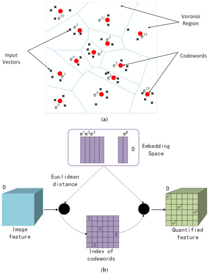
Figure 1.
Vector quantization (VQ) diagram. (a) Embedded codewords in a two-dimensional space. Input vectors are marked with an x, codewords are marked with red circles, and the Voronoi regions are separated with blue boundary lines. (b) The example of VQ applied to image. The blue cube is the input image feature with D dimensions, the green cube is the quantified feature, the purple matrix is the index of codewords, and the embedded codebook is in the purple box.
1.3. The Proposed Method
Due to the capacity for quantification and unsupervised clustering using VQ, we introduced the VQ model on the basis of the CNN model, which effectively solves the problem that CNN cannot be trained in an unsupervised way. The entire unsupervised classification model is named Vector Quantization Clustering with a Convolutional Autoencoder (VQC-CAE). On the one hand, it solves the problem of ignoring the dependency between adjacent pixels when extracting features; on the other hand, it avoids the problem of the previous CNN models, which require labeled data for training.
In the rest of this article, the experimental datasets and basic data preprocessing of PolSAR are introduced, and the proposed unsupervised classification method is described. Then, we show the visual experimental results and accuracy. Then, a discussion of the results is presented, and we end by summarizing the full article.
2. Materials and Methods
2.1. Dataset
Three kinds of data from different sensor platforms were used in this work. The parameters of the data are shown in Table 1. The first kind of data was the C band San Francisco data of RadarSat2 from the spaceborne platform, and the data were acquired on 9 April 2008. The data is obtained from https://ietr-lab.univ-rennes1.fr/polsarpro-bio/san-francisco/ on 30 September 2020. The size of the images was , and the range resolution was 3 m. The data product format was full polarization single look complex data. The second kind of data was L-band German Oberpfaffenhofen data from the E-SAR system of the airborne platform, and the data were acquired on 16 August 1989. The size of the images was , the range resolution was 2 m, and the data product format was full polarization coherence matrix T. The third kind of data was L-band “The Netherlands Flevoland” data from the AIRSAR system of the airborne platform. The size of the images was , and the range resolution was m. The data product format was full polarization coherence matrix T. The last two data sets are obtained from https://earth.esa.int/web/polsarpro/data-sources/sample-datasets/ on 16 November 2020. The geographic range of the three experimental data sets is shown on a map in Figure 2, where (a) shows the San Francisco region and the red box in the right picture is the first experimental data set. Its geographic range is W∼122.5W and 37.75N∼37.85N; (b) is the Oberpfaffenhofen area in Germany, and the red box in the right picture is experimental data set 2. Its geographical range is 11.26E∼11.29E and 48N∼48.1N; and (c) is the Flevoland area in The Netherlands, and the red box in the right picture is experimental data set 3. Its geographical range is 5.3E∼5.43E and 52.29N∼52.41N.

Table 1.
Experimental data parameters.
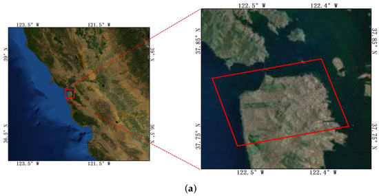
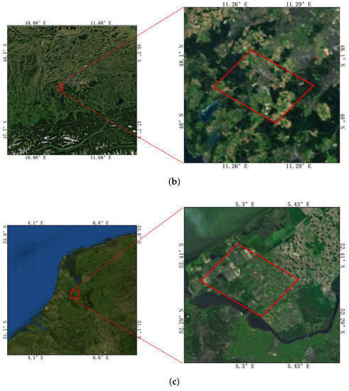
Figure 2.
Geographical extent of the two experimental regions. (a) The San Francisco region, and the red box in the right picture shows experimental data set 1. (b) The Oberpfaffenhofen area in Germany, and the red box in the right picture shows experimental data set 2. (c) The Flevoland area in The Netherlands, and the red box in the right picture shows experimental data set 3.
2.2. Polarimetric SAR Data Preprocessing
The Sinclair complex scattering matrix is normally used to represent the physical scattering characteristics of target pixels for the single look complex (SLC) data of fully polarimetric SAR. The scattering matrix S can be expressed as Equation (1).
where , , and are the scattering elements of four independent polarization channels, and H and V are horizontal polarization and vertical polarization, respectively. Under the condition of single station reciprocity, , the polarization scattering matrix is simplified to the target vector k under the Pauli basis, and k is expressed as Equation (2). The square of two norms of the three elements of the k vector , , are used as three channels of RGB image to synthesize the Pauli pseudo-color image.
In addition, when the fully polarimetric SAR data are given in the form of a coherent matrix T, the coherent matrix T has the following relationship with the Pauli basis vector k, and the expression is as follows: where the superscript H represents the conjugate transposition of vector k. Obviously, the coherent matrix T is a Hermitian matrix whose diagonal elements are real numbers, and the non-diagonal elements are complex numbers. From Equation (3), we can see that , , , meaning that we can synthesize the diagonal elements of the T matrix into a Pauli pseudo-color image.
Figure 3 shows a flowchart of the polarization data preprocessing. When the original data are single look complex (SLC) data, we extract them into a scattering matrix S, and S is decomposed into three scattered components by Pauli decomposition; then, we synthesize the three components to an RGB Pauli pseudo-color image. When the original data are a polarization coherence matrix (T), we extract the diagonal elements of T and then synthesize them into an RGB Pauli pseudo-color image. Finally, the values of all pixels in the pseudo-color image are normalized to , which then are fed into the VQC-CAE network (the method proposed in this paper) to train.
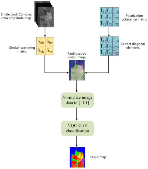
Figure 3.
Flow chart of polarimetric SAR data preprocessing. There are two input sources: single look complex images and coherence matrix.
2.3. Convolutional Autoencoder (CAE)
The convolutional autoencoder (CAE) network includes an encoder network and a decoder network which is realized with multiple convolutional layers and activation functions. The encoder can extract the high-level semantic features of the input image and then use the decoder to reconstruct the input image with the features extracted by the encoder. The reconstruction loss between the reconstructed image and input image are used to supervise the image feature learning process. The encoder first uses a linear mapping and the following nonlinear mapping transformation on the input samples to obtain the feature representation z, and the sample set is expressed as . Equation (4) shows the process of generating latent features after data X through the encoder part. and , respectively, represent the weight and bias parameters of the convolution kernel in the encoder, and f is the activation function after convolutional layers. The decoder is used to perform linear mapping and nonlinear mapping transformation on the hidden latent representation z, remapping it to the original data space to obtain the reconstructed data , as shown in Equation (5), where and are the weight and bias parameters of the convolution kernel in the decoder, and g represents the activation function before output. As shown in Equation (6), the Mean Square Error (MSE) is used as reconstruction loss and the network is optimized with the backpropagation (BP) algorithm.
2.4. Unsupervised Classification Model: Vector Quantization Clustering with Convolutional Autoencoder (VQC-CAE)
The overview of the proposed VQC-CAE model is shown in Figure 4. The input data are the three-channel Pauli pseudo-color images with a size of ; we first use the convolutional autoencoder network (described in the red dashed box) to extract the image features in an unsupervised way. In order to cluster each pixel of the image when performing feature embedding with VQ later, our encoder does not use four convolution kernels without a down-sampling process; it outputs the feature maps with the same size as the input image as , and the dimension of feature maps is D. After that, we use the VQ (the purple dashed box in Figure 4) to quantize the continuous feature maps extracted by the encoder. The embedding space maintains a vector table , as shown in the purple dashed box. The size of the embedding vector table is , where K is the number of table E and D is the dimension of table E, which is the same as the output dimension of the encoder. When the continuous features learned by the encoder are fed into the Vector Quantization model, it performs a nearest neighbor search according to the randomly initialized embedding space vector table (clustering center). The search process is determined by the distance between the input data and the embedding vector table E, and the criterion of the nearest neighbor search is carried out according to Equation (7); the embedded vector obtained by searching is used to replace the input data to obtain the quantized features whose value is a vector from the vector table E. At the same time, each embedding vector corresponds to an integer index between 1 and K in the embedding table. Thus, each embedding vector can represent a cluster center, where index i means that each data can be assigned to one kind of the K categories. In the training process, the updating of the embedding vector table is carried out using the exponential moving average algorithm (EMA) [31], as shown in Equations (8)–(10). When a certain vector in the embedding table is trained to step t, it is updated by weighting the value of the input data closest to it at step t and the last vector value at step . is the number of vectors in the embedding table used for quantifying clustering, is the total value of the vector weighted at the previous moment and is the discount factor.
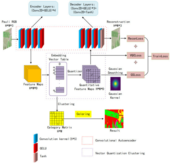
Figure 4.
Framework of Vector Quantization Clustering with Convolutional Autoencoder for unsupervised PolSAR image classification. The convolutional autoencoder composed of a CNN is shown in the red dashed box, the blue rectangular block represents the two-dimensional convolutional layer with the size of , the red rectangular block represents the activation function , and the yellow block represents the output layer activation function . The VQ feature embedding is shown in the purple dashed box, the embedding vector table maintains KD-dimensional vectors. After the feature map passes VQ, a quantitative feature feature map and a category matrix are obtained.
Therefore, the feature embedding from to is a clustering process. As a result, VQ generates both a quantized feature map of size and a K-way category matrix of . Therefore, when the model is trained to converge, the category matrix can be colored according to the categories of ground objects to obtain the final classification. The quantized features are sent to the decoder to reconstruct the original image. At the same time, in order to ensure the continuity of the features learned by the encoder in the spatial domain after quantization and reduce the influence of noise on feature learning, we designed a two-dimensional Gaussian kernel function with a radius of R and a smoothness parameter (variance) to smooth the quantized features and used the loss as an auxiliary loss to supervise the encoder and the quantizer. The total training loss function of the VQC-CAE model is shown in Equation (11). It includes three parts: the first term is the reconstruction loss, which represents the negative log likelihood of the reconstructed image, and it uses the MSE between all the pixels of the input image and reconstructed image pixels as the loss in the Equation (12), which is used to optimize the decoder and encoder, where N is the total number of pixels after feature flattening; the second term is the quantized clustering error, which uses the loss between the continuous feature map and the quantized feature map as the optimization target. In Equation (13), means the stop gradient, which does not work in the forward propagation network. Only in the process of backward propagation is the gradient of the quantized variable no longer forwarded, which is done to achieve the training the of only the encoder. The goal of this is approach to prevent the output of the encoder from frequently jumping across the vectors in the vector table when clustering. The third term in Equation (14) is the Gaussian smoothing loss, and is the feature smoothed by the Gaussian filter.
2.5. Evaluation Index of Classification Accuracy in Polarimetric SAR Images
The classification accuracy evaluation of the polarimetric SAR images is performed by evaluating the accuracy of the classification results based on the ground truth of the SAR image. We used three evaluation indicators in total, including the overall accuracy , average accuracy and coefficient [15,32], which are widely used in the evaluation of classification performance and can evaluate the global classification accuracy in remote sensing images. The confusion matrix was calculated by comparing the classification result with the corresponding ground truth. For the C categories classification problem, the confusion matrix M was a matrix, expressed as Equation (15), in which the element represents the number of samples in which the actual object category i is classified as the category j. According to the confusion matrix M, we can calculate the accuracy of each category, as well as the , and coefficient.
Overall accuracy can reflect the probability that the remote sensing image classification result is consistent with the ground truth of the object. The calculation formula is shown in Equation (16). It can be seen that only diagonal elements can affect the overall accuracy, which is not sufficient to completely judge the classification. Average accuracy can reflect the average probability that each category after classification is consistent with the ground truth of the object, and the calculation formula is shown in Equation (17).
The coefficient was also used to evaluate the classification accuracy and to verify the consistency between the remote sensing classification result and the ground truth of the object. The coefficient can reflect the error of the overall remote sensing image classification. The calculation formula is shown in Equation (18), where N is the total number of samples.
3. Results
3.1. Experimental Model Parameters and Comparison Method
3.1.1. Model Parameters
All the parameters of our model were as follows: the encoder and decoder both used four-layer Conv2D convolution, and each layer of convolution of the encoder was followed by an activation function GELU. The GELU activation function replaced Relu in order to make the model converge quickly. The activation function of the last layer of the decoder after convolution was Tanh, which was used to keep the reconstructed data consistent with the input data between . The size of the convolution kernel was , stride = 1 and padding = 2, the number of channels of the encoder convolutional layer was [128,128,128,3], and the number of channels of the decoder convolutional layer was [128,128,128,3]. The size of the vector quantization embedding table was , where K is the number of cluster centers (eight) and D refers to three dimensions, which was the same as the encoder output dimension. Gaussian smoothing kernel parameters were an R of 15 and of 25.0. The discount factor was 0.95 in Equations (8) and (9) when using EMA to update the vector table. The weights of the and of the in Equation (11) were constrained between [0, 1]. The value of was 0.25 and that of was 0.1 in our experiment. The Adam optimizer was used for gradient descent during model training. The initial learning rate was 0.0002, and we used cosine annealing descent for learning rate decay. The model of our experiment was built and trained in the Pycharm compiler and pytorch deep learning environment on a 2.90 Ghz computer with 8.00 GB RAM, an NVIDIA RTX3080 GPU (10.00 GB memory) and a Core i7-10700F CPU (8 cores).
3.1.2. Comparison Method
In addition, we used the classical H/alpha-Wishart algorithm as our comparison method. When the H/alpha-Wishart method is used to classify SAR images, the coherence matrix T is used as its input, which is different from our method. Usually, PolSAR data need to be processed for multi-view or filter. The purpose of this is to reduce the impact of coherent speckle noise; thus, we used the refined Lee filter in this article. The flowchart of H/alpha-Wishart classification is shown in Figure 5, where the original data are SLC data, which were extracted into a scattering matrix S, and we used S to calculate T with Equation (3). Then, we put the coherence matrix T into a refined Lee filter, and the output of the filter was taken to perform H/alpha decomposition to obtain the initial classification. Finally, Wishart clustering was used to obtain the result map.
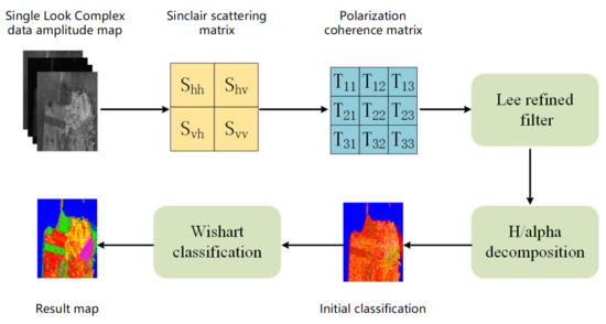
Figure 5.
Flow chart of H/alpha-Wishart classification.
3.2. Experiment Results
3.2.1. RadarSat2 Dataset Experiment Results
The San Francisco area of RadarSat2 was selected as data set 1. Figure 6 shows the original input image of the San Francisco data and the ground truth. The image size was pixels. In the figure, (a) is the Pauli pseudo color image, synthesized by three scattering mechanisms; (b) is the ground truth of (a), where 1,804,087 pixels are marked in the whole image of the ground truth—In total, five objects are included: water, vegetation (VEG), high-density urban (HDU), low-density urban (LDU) and developed (DEV); and (f) is the color set for the five objects, where water is blue, vegetation is green, high-density urban is red, low-density urban is yellow, developed is magenta and the unlabeled pixels are set as black.
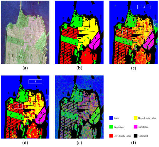
Figure 6.
Experimental data of San Francisco area, ground truth of the ground object and classification results by proposed method and comparison method. Rectangles A, B and C are the specific comparative analysis areas of the classification maps in (c,d). (a) Pauli pseudo color image synthesized by single look complex data. (b) The ground truth of the five objects. (c) The classification result of H/alpha-Wishart. (d) The classification result of the VQC-CAE model. (e) The classification result of the VQC-CAE model without Gaussian smoothing loss. (f) The color set of the ground truth: blue for water, green for vegetation (VEG), red for high-density urban (HDU), yellow for low-density urban (LDU), magenta for developed (DEV) and the unlabeled pixels are black.
In the experiment, we compared our VQC-CAE model with the H/alpha-Wishart algorithm. The classification results after coloring are shown in Figure 6c,d, where (c) is the result of H/alpha-Wishart, (d) is the result of the VQC-CAE model and (e) is the result of the VQC-CAE model without Gaussian smoothing loss. The results of the experiment were processed according to the ground truth, and we masked the pixels in the unlabeled area to black in order to be consistent with the ground truth. First of all, comparing the two classification results from (c) and (d), it can be seen that the five types of objects were all distinguished. The classical H/alpha-Wishart classification results were trivial; there are many cases where there were multiple classification categories in a small area that should have been the same type of object. However, the classification result of our method for each type of object was relatively continuous, because it considered the influence of the spatial neighbors on the central pixel. In addition, the Gaussian smoothing filter was added. Thus, there was no situation in which multiple object categories appeared in a small area. For example, in the area of box A, whose category should be water (blue), the H/alpha-Wishart distinguished it as red (high-density urban) and green (vegetation). In the area of box B, the red areas (high-density urban) were misclassified to a large amount of yellow (low-density urban) areas. In the area of box C, a large area that should have been water was categorized as green (vegetation). This can also be seen from the red oval box in the confusion matrix in Figure 7. Confusion Matrix M1 was from comparison method H/alpha-Wishart and M2 was from the proposed VQC-CAE method. The number of pixels in category 1 divided into 2 reached 28,292, which was much larger than the total of 171 from our method. This indicates that the H/alpha-Wishart algorithm has certain shortcomings: it can not completely distinguish categories only with polarization decomposition, which reflects its target scattering characteristics. However, the classification model based on feature extraction and clustering in this paper can extract high-level semantic information of objects, and the misclassification of large areas did not occur. In addition, we present the classification results of the model without Gaussian smoothing loss in Figure 6e. In contrast with (d), it can be seen that the lack of Gaussian smoothing loss made the classification results very different. There was a large amount of noise on the classification map, and both low-density urban and developed areas were not classified. This also shows that the Gaussian smoothing loss was necessary when training the unsupervised classification model in this article.
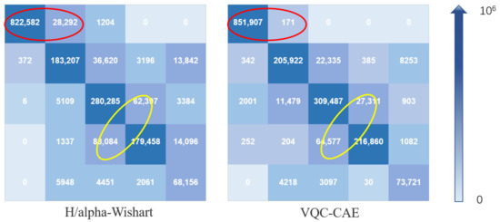
Figure 7.
Confusion matrix of H/alpha-Wishart method and VQC-CAE model. The categories from the first row to the fifth row are water, vegetation, high-density urban, low-density urban and developed. The blue gradient arrow represents the difference of confusion matrix element values from 0 to ; the larger the matrix element value, the darker the color. The larger the value of the non-diagonal element in the confusion matrix, the easier it is to classify pixels from other categories into this category. The larger the diagonal element, the smaller the misclassification of the category.
In addition, we performed a statistical analysis on the classification accuracy of each object based on all the marked pixels of the object on the ground truth of images in this experiment. According to the confusion matrix, the classification accuracies of each type of object were calculated, alongside the three indicators of , and , as shown in Table 2. The table shows that the classification accuracies of the proposed method in this paper and the traditional H/alpha-Wishart method were more than 99% in the water category, but in the remaining four types of ground objects, the method proposed in this paper performed much better than the comparison method: the accuracy of vegetation reached 92.76% which was 11% higher than the comparison method. The lowest classification accuracy was for the category high-density urban, but it also reached 77.47%, higher than the value of 68.25% of the comparison method. In addition, the three classification accuracy indicators of , and reached 91.87%, 89.27% and 88.28%, which were 5% to 10% higher than the comparison method.
Table 2.
Comparison of the classification accuracy of our approach with other methods.
3.2.2. E-SAR Dataset Experiment Results
The Oberpfaffenhofen area in Germany presented by E-SAR was selected as data set 2. Figure 8 shows the original input image of the San Francisco data and its ground truth. The image sizes were pixels. In the figure, (a) is the Pauli pseudo color image and (b) is the ground truth of (a), and there are 1,374,298 pixels marked in the whole image of the ground truth. In total, three objects are included: built-up area (Build), wood land (Wood) and open area (Open). (e) is the color set for the objects, where Build is red, Wood is green, Open is yellow and the unlabeled pixels are set as black.
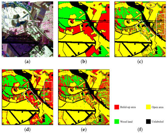
Figure 8.
Experimental data of the Oberpfaffenhofen area, ground truth of the ground object and classification results with the proposed method and comparison method. Rectangles A and B are the specific comparative analysis areas of the classification maps in (c,d). (a) Pauli pseudo color image synthesized by polarimetric coherence matrix T. (b) The ground truth of the three objects. (c) The classification result of H/alpha-Wishart. (d) The classification result of the VQC-CAE model. (e) The classification result of the VQC-CAE model without Gaussian smoothing loss. (f) The color set of the ground truth: green for wood land (Wood), red for built-up area (Build), yellow for open area (Open), and the unlabeled pixels are black.
In the experiment, we compared our VQC-CAE model with the H/alpha-Wishart algorithm. The classification results after coloring are shown in Figure 8c,d. (c) is the result of H/alpha-Wishart and (d) is the result of the VQC-CAE model. The results of the experiment were processed by masked the pixels in the unlabeled area to black according to the ground truth in order to be consistent with the ground truth. First of all, comparing the two classification results, it can be seen that five types of objects were all distinguished. However, the traditional H/alpha-Wishart classification was not able to separate Build and Open areas in the areas of A and B, with most of the pixels of the red built-up area being classified into yellow open areas. On the contrary, the classification with our method of each type of objects was relatively continuous, and in the area of A, most of the pixels of the red (Build) area were classified correctly. This can also be seen from the red oval box of the confusion matrix in Figure 9, Confusion Matrix M1 was from the comparison method H/alpha-Wishart and M2 was from the proposed VQC-CAE method. The number of pixels in category 1 divided into category 3 reached 115,106 which is almost four times the total of 26,843 from our method. At the same time, it can be seen from the purple oval boxes in the confusion matrix that the numbers of pixels in the second category divided into the first category were 60,676 and 57,708 respectively, which are similar. For the proposed VQC-CAE method, the number of pixels in the third category divided into the first category was 70,886, which is much larger than the score of 11,249 for the comparison method. This can also be seen from the purple oval areas in (c) and (d) in Figure 8. This shows that our method exhibited some deviations in the classification of the open areas in this oval area. In addition, we present the classification results of the model without Gaussian smoothing loss in Figure 8e. In contrast with (d), it can be seen that the lack of Gaussian smoothing loss made the classification results very different. The two categories of green (wood land) and red (built-up) areas were mixed together, and they were almost indistinguishable. The whole classification map has large amounts of noise. Thus, the Gaussian smoothing loss is necessary when training to reduce the influence of noise and obtain better classification results.
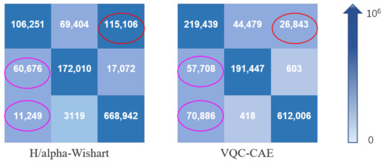
Figure 9.
Confusion matrix of thhe H/alpha-Wishart method and VQC-CAE model. The categories from the first row to the third row are built-up area, wood land and open area. The blue gradient arrow on the right represents the difference of confusion matrix element values from 0 to ; the larger the matrix element value, the darker the color. The larger the value of the non-diagonal element in the confusion matrix, the easier it is to classify pixels from other categories into this category. The larger the diagonal element, the smaller the misclassification of the category.
In addition, we performed a statistical analysis on the classification accuracy of each object based on all the labeled pixels on the ground truth of images in this experiment. According to the confusion matrix, the classification accuracy of each type of object was calculated, and the three indicators of , and are shown in Table 3. This shows that the method proposed in this paper performed better than the comparison method in the classification of wood land and open area; the classification accuracy of our method for wood land was 11% better than comparison method, and the classification accuracy for open area reached 95.71%, which is much higher than the score of 83.5% for the comparison method. The classification accuracy of the built-up area was the lowest, but it was also nearly 4% higher than the comparison method. In addition, from a holistic perspective, the values of , and were much higher than the comparison method, and the OA was 83.58%, which was higher than the comparison method by 5%; furthermore, the coefficient of the proposed method also reached 72.69% while the comparison method scored less than 60%.
Table 3.
Comparison of the classification accuracy of our approach with other methods.
3.2.3. AIRSAR Dataset Experiment Results
The Flevoland area in The Netherlands presented by AIRSAR was selected as data set 3. Figure 10 shows the original input image of the Flevoland data and its ground truth. The image size was pixels. In the figure, (a) is the Pauli pseudo color image, synthesized by three scattering mechanisms, and (b) is the ground truth of (a), where 25,282 pixels are marked in the whole image of the ground truth. In total, six objects are included: peas, Lucerne, beet, potatoes, soil and wheat. Additionally, (e) is the color set for the six objects, where peas is light blue, Lucerne is navy blue, beet is pink, potatoes is orange, soil is brown, wheat is light green, and the unlabeled pixels are set as black.
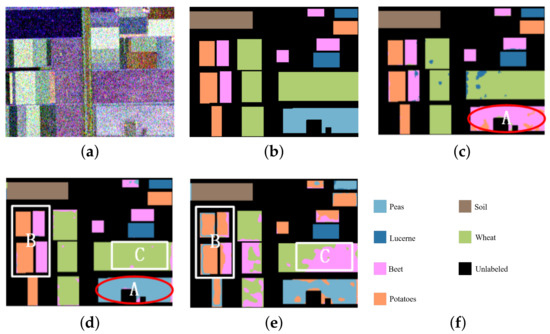
Figure 10.
Experimental data of the Flevoland area, ground truth of the ground object and classification results by the proposed method and comparison method. Ellipse A, Rectangles B and C are the specific comparative analysis areas of the classification maps in (c–e). (a) Pauli pseudo color image synthesized by the polarimetric coherence matrix T. (b) The ground truth of the three objects. (c) The classification result of H/alpha-Wishart. (d) The classification result of the VQC-CAE model. (e) The classification result of the VQC-CAE model without Gaussian smoothing loss. (f) The color set of the ground truth: light blue for peas, navy blue for Lucerne, pink for beet, orange for potatoes, brown for soil, light green for wheat, and the unlabeled pixels are black.
In the experiment, we compared our VQC-CAE model with the H/alpha-Wishart algorithm. The classification results after coloring are shown in Figure 10c,d, where (c) is the result of H/alpha-Wishart, (d) is the result of the VQC-CAE model. The results of the experiment were processed by masking the pixels in the unlabeled area to black according to the ground truth in order to be consistent with the ground truth. First of all, comparing the two classification results, it can be seen that the six types of objects were all distinguished by VQC-CAE. However the traditional H/alpha-Wishart classification was not able to separate light blue (peas) from pink (beet) in the area of A, as all the pixels of peas were mixed into beet. On the contrary, each type of objects was distinguished with our approach. This can also be seen from the red oval box of the confusion matrix in Figure 11, Confusion Matrix M1 was from the comparison method H/alpha-Wishart and M2 was from the proposed VQC-CAE method. The number of pixels in category 1 divided into category 3 reached 3434, and no pixels are classified into the first category in yellow oval box. At the same time, it can be seen from the purple oval boxes in the confusion matrix that only the fifth number in the fifth column had a value other than 0, which means that the classification accuracy obtained from the two methods for the fifth category of soil was 100%. In addition, we present the classification results of the model without Gaussian smoothing loss in Figure 10e. In contrast with (d), it can be seen in areas B and area C that the lack of Gaussian smoothing loss meant that the model could not distinguish pink (beet) and light green (wheat) areas, and several categories were mixed together.
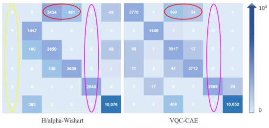
Figure 11.
Confusion matrix of H/alpha-Wishart method and the VQC-CAE model. The categories from the first row to the sixth row are peas, Lucerne, beet, potatoes, soil and wheat. The blue gradient arrow on the right represents the difference of confusion matrix element values from 0 to ; the larger the matrix element value, the darker the color. The larger the value of the non-diagonal element in the confusion matrix, the easier it is to classify pixels from other categories into this category. The larger the diagonal element, the smaller the misclassification of the category.
In addition, we performed a statistical analysis on the classification accuracy of each object based on all the labeled pixels on the ground truth of images in this experiment. According to the confusion matrix, the classification accuracy of each type of object was calculated, and the three indicators of , and are shown in Table 4. This shows that the method proposed in this paper performed better than the comparison method in the classification of all the objects. The classification accuracy of our method for peas was 98.20%, but that of H/alpha-Wishart was 0 because the category peas was misclassified as beet, which also caused the accuracy of beet to be only 44.59%. The accuracy for beet with the proposed method was 82.66%. In addition, from a holistic perspective, the values of , and were much higher than the comparison method, and the OA was 96.93%, which was higher than the comparison method by 15%; the coefficient of the proposed method also reached 95.95%, and the comparison method was less than 80%.
Table 4.
Comparison of classification accuracy with other methods.
3.2.4. Analysis of Classification Maps with Post-Processing
Due to the poor robustness of the basic H/alpha-Wisahrt classification method to noise, speckle noise exists on the three classification maps shown in Figure 12a,c,e. Therefore, the post-processing operation of the classification map needed to be performed. Inspired by the smoothing filtering in [33], we used a mean filter with a window size of to perform sliding window filtering on the classification map. We conducted experiments on the values of window sizes w from 3 to 25 and found that the best filtering effect could be obtained when w was 15. Thus, we give the post-processing results of the classification map when w was 15 in Figure 12b,d,f. Comparing the left and right classification maps of the three data sets, respectively, it can be found that many noise points have been eliminated. In addition, we show the classification accuracy after post-processing in Table 2, Table 3 and Table 4. It can be found that the mean filter improved the classification accuracy of San Francisco and Flevoland data sets. The OAs of the two data sets increased from 85.01% and 81.79% to 90.10% and 83.02%, respectively, but these were still lower than the scores of 91.8% and 96.93% for the proposed VQC-CAE method. For Oberpfaffenhofen data, the large amount of misclassification led to more category confusion and reduced the classification accuracy after filtering, and the OA decreased from 77.40% to 77.07%.
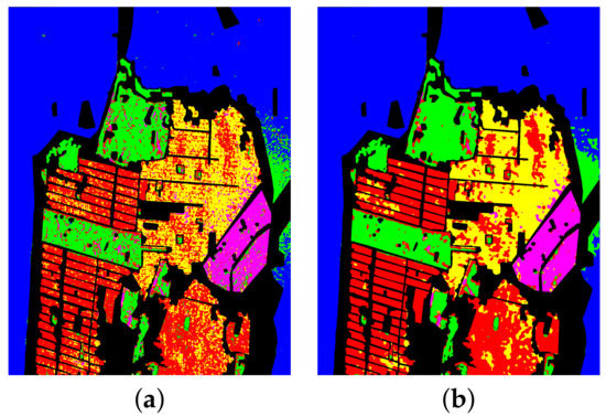
Figure 12.
Comparison of basic H/alpha-Wishart classification map and post-processed classificationmap with mean filter. (a) The classification result of H/alpha-Wishart (basic) for San Francisco.(b) The classification result of the basic approach with a mean filter for San Francisco. (c) Theclassification result of H/alpha-Wishart (basic) for Oberpfaffenhofen. (d) The classification result ofthe basic approach with a mean filter for Oberpfaffenhofen. (e) The classification result of H/alpha-Wishart (basic) for Flevoland. (f) The classification result of the basic approach with a mean filterfor Flevoland.
4. Discussion
In this paper, we first analyzed the classical unsupervised classification algorithms for SAR images. These methods use polarization decomposition and feature decomposition to extract the features of an image and then use clustering methods such as K-means or Wishart to implement clustering. Because the correlation between neighboring pixels is not considered in the feature extraction, the classification result is imprecise, with salt and pepper noise, and the classification accuracy is not high. Then, we considered the CNN model for classification; it extracts semantic information of images and can capture the non-linear dependency between adjacent pixels. The classification accuracy is much higher, but it requires labeled data during training, and the model has high complexity. Thus, we introduced the VQ into the feature stage on the basis of CNN so that the whole model could be trained in a fully unsupervised way. This approach can train the process of feature extraction and clustering simultaneously. In addition, the Gaussian smoothing filter was added after the VQ to further eliminate the influence of image noise and obtain better classification results. The three experiments proved that the classification accuracy of our model was much higher than the H/alpha-Wishart algorithm. It can also be seen from the visualized classification map that the classification of each object area was relatively continuous without salt and pepper noise. However, as shown in the yellow oval box of the classification confusion matrix in Figure 7, there were many misclassified pixels between category 3 and category 4; that is, the classifications of high-density urban and low-density urban building still showed shortcomings, which is also an important impacting factor on the overall classification accuracy of this method. We consider that the reason for this result is that the similarity between these two types of objects is very high. In addition, using only Pauli pseudo-color images as an input may lead to a lack of sufficient object information. Therefore, the classification of image features that incorporate polarization decomposition, feature decomposition and grayscale texture as the input of the VQC-CAE model may improve the classification accuracy. More importantly, comparing (d) and (e) in Figure 6 and Figure 8, respectively, it can be found that if Gaussian smoothing loss is not used for auxiliary training after using VQ for feature embedding, there will be a large amount of noise in the classification result, and targets with similar features such as high-density urban and low-density urban areas will therefore be difficult to distinguish.
5. Conclusions
This paper proposes a novel unsupervised classification network model named VQC-CAE for fully PolSAR images. The proposed method has creative significance for unsupervised classification applications. Compared with the H/alpha-Wisahrt algorithm, it not only considers the correlation of the neighborhood but also has good robustness to speckle noise. We have performed experiments on three real PolSAR data sets to verify the performance of the model. The results show that the proposed method can obtain a more continuous classification map and the classification accuracy and coefficient are both much higher than that of the comparison method. In addition, although the post-processing of mean filtering was performed for the comparison method, the classification accuracy of the proposed method was better, which also shows that the VQC-CAE method has better noise suppression ability.
Future work can be carried out in the following directions: on one hand, we can use only single-polarization or dual-polarization data to verify the applicability of this deep vector quantization clustering model; on the other hand, we can try to use K-means or other clustering methods instead of the EMA algorithm as a vector table update strategy when performing VQ clustering to verify classification accuracy.
Author Contributions
Conceptualization, Y.Z. (Yixin Zuo); Formal analysis, Y.Z. (Yixin Zuo); Funding acquisition, Y.H.; Investigation, Y.Z. (Yueting Zhang); Project administration, Y.Z. (Yixin Zuo) and M.W.; Resources, J.G.; Supervision, B.L.; Writing—original draft, Y.Z. (Yixin Zuo); Writing—review & editing, Y.Z. (Yixin Zuo). All authors have read and agreed to the published version of the manuscript.
Funding
This research was funded by the National Key Research and Development Program with grant number 2018YFC1407201.
Conflicts of Interest
The authors declare no conflict of interest.
References
- Cloude, S. Polarisation: Applications in Remote Sensing; Oxford University Press: Oxford, UK, 2009. [Google Scholar]
- Van Zyl, J.J. Unsupervised classification of scattering behavior using radar polarimetry data. IEEE Trans. Geosci. Remote Sens. 1989, 27, 36–45. [Google Scholar] [CrossRef]
- Cloude, S.R.; Pottier, E. An entropy based classification scheme for land applications of polarimetric SAR. IEEE Trans. Geosci. Remote Sens. 1997, 35, 68–78. [Google Scholar] [CrossRef]
- Lee, J.S.; Grunes, M.R.; Ainsworth, T.L.; Du, L.; Schuler, D.L.; Cloude, S.R. Unsupervised classification using polarimetric decomposition and complex Wishart classifier. In Proceedings of the IGARSS ’98, Sensing and Managing the Environment 1998 IEEE International Geoscience and Remote Sensing. Symposium Proceedings (Cat. No.98CH36174), Seattle, WA, USA, 6–10 July 1998. [Google Scholar]
- Goodman, N.R. Statistical Analysis Based on a Certain Multivariate Complex Gaussian Distribution (an Introduction). Ann. Math. Stat. 1963, 34, 152–177. [Google Scholar] [CrossRef]
- Lee, J.S.; Grunes, M.R.; Pottier, E.; Ferro-Famil, L. Unsupervised terrain classification preserving polarimetric scattering characteristics. IEEE Trans. Geosci. Remote Sens. 2004, 42, 722–731. [Google Scholar]
- Guo, S.; Tian, Y.; Yang, L.; Chen, S.; Wen, H. Unsupervised classification based on H/alpha decomposition and Wishart classifier for compact polarimetric SAR. In Proceedings of the 2015 IEEE International Geoscience and Remote Sensing Symposium (IGARSS), Milan, Italy, 26–31 July 2015. [Google Scholar]
- Shi, Y.; Lei, M.; Ma, R.; Niu, L. Learning Robust Auto-Encoders with Regularizer for Linearity and Sparsity. IEEE Access 2019, 7, 17195–17206. [Google Scholar] [CrossRef]
- Long, J.; Shelhamer, E.; Darrell, T. Fully Convolutional Networks for Semantic Segmentation. IEEE Trans. Pattern Anal. Mach. Intell. 2015, 39, 640–651. [Google Scholar]
- Ronneberger, O.; Fischer, P.; Brox, T. U-Net: Convolutional Networks for Biomedical Image Segmentation. In Proceedings of the International Conference on Medical Image Computing and Computer-Assisted Intervention, Munich, Germany, 5–9 October 2015; Springer International Publishing: Cham, Switzerland, 2015. [Google Scholar]
- Zhao, H.; Shi, J.; Qi, X.; Wang, X.; Jia, J. Pyramid scene parsing network. In Proceedings of the 2017 IEEE Conference on Computer Vision and Pattern Recognition, Honolulu, HI, USA, 21–26 July 2017; pp. 2881–2890. [Google Scholar]
- Chen, L.C.; Papandreou, G.; Kokkinos, I.; Murphy, K.; Yuille, A.L. Semantic image segmentation with deep convolutional nets and fully connected crfs. Comput. Sci. 2014, 357–361. [Google Scholar]
- Chen, L.C.; Papandreou, G.; Kokkinos, I.; Murphy, K.; Yuille, A.L. Deeplab: Semantic image segmentation with deep convolutional nets, atrous convolution, and fully connected crfs. IEEE Trans. Pattern Anal. Mach. Intell. 2018, 40, 834–848. [Google Scholar] [CrossRef] [PubMed]
- Chen, L.C.; Papandreou, G.; Schroff, F.; Adam, H. Rethinking atrous convolution for semantic image segmentation. arXiv 2017, arXiv:1706.05587. [Google Scholar]
- Ding, A.; Zhou, X. Land-Use Classification with Remote Sensing Image Based on Stacked Autoencoder. In Proceedings of the International Conference on Industrial Informatics-Computing Technology, Wuhan, China, 3–4 December 2016. [Google Scholar]
- Sun, Z.; Li, J.; Liu, P.; Cao, W.; Gu, X. Sar image classification using greedy hierarchical learning with unsupervised stacked caes. IEEE Trans. Geosci. Remote Sens. 2020, 1–19. [Google Scholar] [CrossRef]
- Masci, J.; Meier, U.; Dan, C.; Schmidhuber, J. Stacked Convolutional Auto-Encoders for Hierarchical Feature Extraction. In Proceedings of the International Conference on Artificial Neural Networks, Espoo, Finland, 14–17 June 2011; Springer: Berlin/Heidelberg, Germany, 2011. [Google Scholar]
- Xu, C.; Sui, H.; Liu, J.; Sun, K.; Hua, L. Unsupervised Classification of High-Resolution SAR Images Using Multilayer Level Set Method. In Proceedings of the IGARSS 2019—2019 IEEE International Geoscience and Remote Sensing Symposium, Yokohama, Japan, 28 July–2 August 2019. [Google Scholar]
- Ferro-Famil, L.; Pottier, E.; Lee, J.S. Unsupervised classification of multifrequency and fully polarimetric sar images based on the h/a/alpha-wishart classifier. IEEE Trans. Geosci. Remote Sens. 2001, 39, 2332–2342. [Google Scholar] [CrossRef]
- Nogueira, F.; Marques, R.; Medeiros, F. Sar image segmentation based on unsupervised classification of log-cumulants estimates. IEEE Geosci. Remote Sens. Lett. 2020, 17, 1287–1289. [Google Scholar] [CrossRef]
- Yu, P. Unsupervised polarimetric sar image segmentation and classification using region growing with edge penalty. IEEE Trans. Geosci. Remote Sens. 2012, 50, 1302–1317. [Google Scholar] [CrossRef]
- Kayabol, K.; Gunsel, B. Unsupervised classification of sar images using normalized gamma process mixtures. Digit. Signal Process. 2013, 23, 1344–1352. [Google Scholar] [CrossRef]
- Liu, X.; Jiao, L.; Tang, X.; Sun, Q.; Zhang, D. Polarimetric convolutional network for polsar image classification. IEEE Trans. Geosci. Remote. Sens. 2019, 57, 3040–3054. [Google Scholar] [CrossRef]
- He, C.; He, B.; Tu, M.; Wang, Y.; Qu, T.; Wang, D. Fully convolutional networks and a manifold graph embedding-based algorithm for polsar image classification. Remote Sens. 2020, 12, 1467. [Google Scholar] [CrossRef]
- Wang, L.; Xu, X.; Hao, D.; Rong, G.; Pu, F. Multi-pixel simultaneous classification of polsar image using convolutional neural networks. Sensors 2018, 18, 769. [Google Scholar] [CrossRef]
- Chatterjee, A.; Saha, J.; Mukherjee, J.; Aikat, S.; Misra, A. Unsupervised land cover classification of hybrid and dual-polarized images using deep convolutional neural network. IEEE Geosci. Remote Sens. Lett. 2021, 18, 969–973. [Google Scholar] [CrossRef]
- Zhou, Y.; Wang, H.; Xu, F.; Jin, Y.Q. Polarimetric SAR Image Classification Using Deep Convolutional Neural Networks. IEEE Geosci. Remote Sens. Lett. 2017, 13, 1935–1939. [Google Scholar] [CrossRef]
- Ahishali, M.; Kiranyaz, S.; Ince, T.; Gabbouj, M. Multifrequency Polsar Image Classification Using Dual-Band 1D Convolutional Neural Networks. In Proceedings of the 2020 Mediterranean and Middle-East Geoscience and Remote Sensing Symposium (M2GARSS), Tunis, Tunisia, 9–11 March 2020. [Google Scholar]
- Zhang, Z.; Wang, H.; Xu, F.; Jin, Y.Q. Complex-Valued Convolutional Neural Network and Its Application in Polarimetric SAR Image Classification. IEEE Trans. Geosci. Remote Sens. 2017, 55, 7177–7188. [Google Scholar] [CrossRef]
- Chen, S.W.; Tao, C.S. PolSAR Image Classification Using Polarimetric-Feature-Driven Deep Convolutional Neural Network. IEEE Geosci. Remote Sens. Lett. 2018, 15, 627–631. [Google Scholar] [CrossRef]
- Łańcucki, A.; Chorowski, J.; Sanchez, G.; Marxer, R.; Chen, N.; Dolfing, H.J.G.A.; Khurana, S.; Alumäe, T. Antoine Laurent Robust Training of Vector Quantized Bottleneck Models. In Proceedings of the 2020 International Joint Conference on Neural Networks (IJCNN), Glasgow, UK, 19–24 July 2020. [Google Scholar]
- Geng, J.; Jiang, W.; Deng, X. Multi-scale deep feature learning network with bilateral filtering for sar image classification-sciencedirect. ISPRS J. Photogramm. Remote Sens. 2020, 167, 201–213. [Google Scholar] [CrossRef]
- Fernndez-Michelli, J. Unsupervised classification algorithm based on em method for polarimetric sar images. ISPRS J. Photogramm. Remote Sens. 2016, 117, 56–65. [Google Scholar] [CrossRef]


Publisher’s Note: MDPI stays neutral with regard to jurisdictional claims in published maps and institutional affiliations. |
© 2021 by the authors. Licensee MDPI, Basel, Switzerland. This article is an open access article distributed under the terms and conditions of the Creative Commons Attribution (CC BY) license (https://creativecommons.org/licenses/by/4.0/).