
Annually Urban Fractional Vegetation Cover Dynamic Mapping in Hefei, China (1999–2018)


Abstract

1. Introduction
2. Study Area and Datasets
2.1. Study Area
2.2. Datasets
3. Methods
3.1. An Improved Vegetation Index
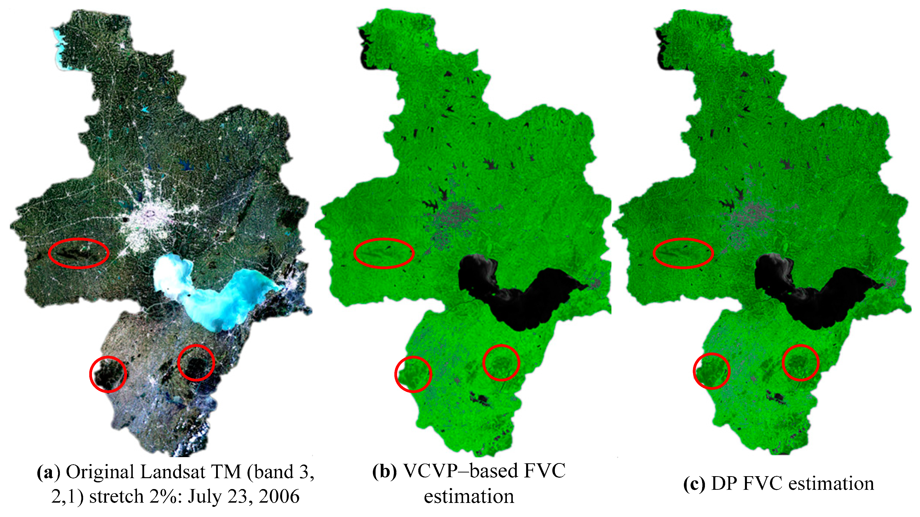
3.2. VCVP–Based FVC Estimation
3.3. Automatic Threshold Selection and ODRVI Model Validation
4. Results
4.1. Performance of the ODRVI Model
4.2. ODRVI Model Validation
4.3. FVC Verification and Estimation
4.4. FVC Dynamic Change Mapping in Hefei (1999–2018)
4.5. Results Analysis of FVC Changes in Hefei (1999–2018)
- (1)
- Continuously rapid decay (1999–2004). The total area of all FVC levels showed a rapid decline, with an average decline rate of 1.76% and a total area decrease of 1380.46 km2. The area of ELF, LF, and MF decreased by 1.06%, 5.63%, and 14.29%, respectively. The area of MHF and HF in the mountains of Hefei increased by 1.15% and 11.83 km2, respectively.
- (2)
- Rapid decline with fluctuations (2005–2008). The total area of all FVC levels decreased by 3883.28 km2 from 2005 to 2008, with an average decrease rate of 7.97%. From 2005 to 2008, the area of MF decreased by 45.03%, and those of LF, MHF, and HF decreased by 11.99%, 14.14%, and 0.19%, respectively.
- (3)
- Fluctuated attenuation (2009–2013). The average vegetation cover area decreased by 382.9 km2 per year, the total area of all FVC levels decreased by 5.45%, and the areas of ELF, LF, and MF decreased by 13.73%, 6.53%, and 1.61%, respectively. The area of HF increased by 0.54%. The changes in the areas of LF and MF occurred in areas surrounding the southwest, southeast, and south of downtown Hefei, and changes in the area of HF were observed in the eastern and southeastern areas.
- (4)
- Fluctuated increase (2014–2018). The overall area of all FVC levels showed an increasing trend (policy intervention factor), and the area increased by 1294.59 km2 in Hefei. The areas of MF, LF, MHF, and HF increased by 10.02%, 1.12%, 4.22%, and 0.19%, respectively. A rapid increase in the area of 1972 km2 occurred from 2015 to 2016. The areas of LF, MF, and MHF increased by 5.76%, 21.21%, and 3.39% in the north and center of downtown Hefei, respectively.
5. Discussion
5.1. Performance of the ODRVI Model
5.2. Influence Factors of the ODRVI Model
5.3. Performance of FVC Estimation
5.4. Influence of Urban Sprawl on FVC Change
- (1)
- Urban development reduced the total area of FVC and increased the fragmentation of vegetation cover areas. The urban area expanded annually, and the fragmentation degree of vegetated areas started to increase as areas surrounding the downtown region were developed, such as in 2010, 2013, and 2014. In addition to seasonal change and weather influences, the increased fragmentation of vegetated areas occurred due to the expansion of the city and human activities.
- (2)
- Urban sprawl changed the spatial distribution of all FVC levels. Urban expansion decreased vegetation cover and changed the area of FVC to different degrees. For example, the area of ELF, LF, and MF decreased by 13.39%, 6.35%, and 1.61%, respectively, in the southwest and southeast areas of Hefei from 2009 to 2013.
- (3)
- Urban sprawl changed the area of all grades of FVC. Urban greening and afforestation slowed down the rate of FVC change to a certain extent. The area increased in the ELF and LF levels. The government deepened its understanding of environmental changes caused by urban development and ensured the protection and conservation of original forests and green spaces. The proportion of MF and HF increased. The proportion of HF increased by 0.18% from 1999 to 2018, and that of MHF increased by 3.4%.
- (4)
- Urban sprawl accelerated urban water pollution and reduced the vegetation cover in the surrounding areas. An increase in the proportion of urban impervious surfaces caused a large amount of surface runoff. Sediment, rich nutrients, pesticides, and garbage entered the water, increasing water pollution and killing vegetation.
6. Conclusions
- (1)
- The ODRVI model was proposed to improve the sensitivity to the water content, roughness degree, and soil type by minimizing the influence of bare soil in areas of sparse vegetation cover. It improved the overall accuracy of vegetation extraction and the ability to distinguish vegetation from non-vegetation.
- (2)
- The ODRVI enhanced the stability of FVC estimation in the near-infrared (NIR) band in areas of dense and sparse vegetation cover. The ODRVI model was verified to have better performance in multi-temporal Landsat images, and obtain higher accuracy than the typical VI models by dynamic threshold adjusting.
- (3)
- An improved FVC estimation method based on the ODRVI model and VCVP-based model was proposed. The VCVP-based FVC estimation had a more stable performance than the DP-based FVC estimation in both high and low density vegetation cover areas, and the classification error was relatively low.
- (4)
- Annual dynamic change mapping of FVC using the VCVP-based FVC estimation model was applied in Hefei over 20 years. The total FVC area had an overall decreasing trend, and the fluctuation change of all FVC grades was observed. The process of the fluctuation FVC change was divided into four stages: Continuous rapid decay (1999–2004), rapid decline with fluctuations (2005–2008), fluctuation attenuation (2009–2013), and fluctuated increase (2014–2018). Urban sprawl played a crucial role in the change of all FVC grades.
Author Contributions
Funding
Institutional Review Board Statement
Informed Consent Statement
Data Availability Statement
Acknowledgments
Conflicts of Interest
References
- Kumar, D.; Scheiter, S. Biome diversity in South Asia-How can we improve vegetation models to understand global change impact at regional level? Sci. Total Environ. 2019, 671, 1001–1016. [Google Scholar] [CrossRef]
- Walker, B.; Steffen, W. An Overview of the Implications of Global Change for Natural and Managed Terrestrial Ecosystems. Conserv. Ecol. 1997, 1, 2. [Google Scholar] [CrossRef]
- Smirnova, O.V.; Toropova, N.A. Potential vegetation and potential ecosystem cover. Biol. Bull. Rev. 2017, 7, 139–149. [Google Scholar] [CrossRef]
- Gao, L.; Wang, X.; Johnson, B.A.; Tian, Q.; Wang, Y.; Verrelst, J.; Mu, X.; Gu, X. Remote sensing algorithms for estima-tion of fractional vegetation cover using pure vegetation index values: A review. ISPRS J. Photogramm. Remote Sens. 2020, 159, 364–377. [Google Scholar] [CrossRef]
- Wang, J.D.; Liang, S.L. Chapter 12—Fractional Vegetation Cover: Advanced Remote Sensing, 2nd ed.; Academic Press: Cambridge, MA, USA, 2020; pp. 477–510. [Google Scholar] [CrossRef]
- Younes, N.; Joyce, K.E.; Northfield, T.D.; Maier, S.W. The effects of water depth on estimating Fractional Vegetation Cover in mangrove forests. Int. J. Appl. Earth Obs. Geoinf. 2019, 83, 101924. [Google Scholar] [CrossRef]
- Tu, Y.; Jia, K.; Wei, X.; Yao, Y.; Xia, M.; Zhang, X.; Jiang, B. A Time-Efficient Fractional Vegetation Cover Estimation Method Using the Dynamic Vegetation Growth Information from Time Series GLASS FVC Product. IEEE Geosci. Remote Sens. Lett. 2020, 17, 1672–1676. [Google Scholar] [CrossRef]
- Liu, Q.; Zhang, T.; Li, Y.; Li, Y.; Bu, C.; Zhang, Q. Comparative Analysis of Fractional Vegetation Cover Estimation Based on Multi-sensor Data in a Semi-arid Sandy Area. Chin. Geogr. Sci. 2018, 29, 166–180. [Google Scholar] [CrossRef]
- Hishe, S.; Lyimo, J.; Bewket, W. Effects of soil and water conservation on vegetation cover: A remote sensing based study in the Middle Suluh River Basin, northern Ethiopia. Environ. Syst. Res. 2017, 6, 26. [Google Scholar] [CrossRef]
- Chen, J.; Yi, S.; Qin, Y.; Wang, X. Improving estimates of fractional vegetation cover based on UAV in alpine grassland on the Qinghai–Tibetan Plateau. Int. J. Remote Sens. 2016, 37, 1922–1936. [Google Scholar] [CrossRef]
- Mu, X.; Song, W.; Gao, Z.; McVicar, T.R.; Donohue, R.J.; Yan, G. Fractional vegetation cover estimation by using mul-ti-angle vegetation index. Remote Sens. Environ. 2018, 216, 44–56. [Google Scholar] [CrossRef]
- Feng, L.; Jia, Z.; Li, Q.; Xu, K. Fractional Vegetation Cover Estimation Based on MODIS Satellite Data from 2000 to 2013: A Case Study of Qinghai Province. J. Indian Soc. Remote Sens. 2016, 44, 269–275. [Google Scholar] [CrossRef]
- Jia, K.; Yang, L.; Liang, S.; Xiao, Z.; Zhao, X.; Yao, Y.; Zhang, X.; Jiang, B.; Liu, D. Long-Term Global Land Surface Satellite (GLASS) Fractional Vegetation Cover Product Derived from MODIS and AVHRR Data. IEEE J. Sel. Top. Appl. Earth Obs. Remote Sens. 2018, 12, 508–518. [Google Scholar] [CrossRef]
- Nguyen, T.T. Fractional Vegetation Cover Change Detection in Megacities Using Landsat Time-Series Images: A Case Study of Hanoi City (Vietnam) During 1986–2019. Geogr. Environ. Sustain. 2019, 12, 175–187. [Google Scholar] [CrossRef]
- Jänicke, C.; Okujeni, A.; Cooper, S.; Clark, M.; Hostert, P.; van der Linden, S. Brightness gradient-corrected hyper-spectral image mosaics for fractional vegetation cover mapping in northern California. Remote Sens. Lett. 2020, 11, 1–10. [Google Scholar] [CrossRef]
- Scanlon, T.M.; Albertson, J.D.; Caylor, K.K.; Williams, C. Determining land surface fractional cover from NDVI and rainfall time series for a savanna ecosystem. Remote Sens. Environ. 2002, 82, 376–388. [Google Scholar] [CrossRef]
- Roberts, D.A.; Dennison, P.E.; Roth, K.L.; Dudley, K.; Hulley, G. Relationships between dominant plant species, frac-tional cover and land surface temperature in a Mediterranean ecosystem. Remote Sens. Environ. 2015, 167, 152–167. [Google Scholar] [CrossRef]
- Coy, A.; Rankine, D.; Taylor, M.; Nielsen, D.C.; Cohen, J. Increasing the accuracy and automation of fractional vegetation cover estimation from digital photographs. Remote Sens. 2016, 8, 474. [Google Scholar] [CrossRef]
- Wang, X.; Jia, K.; Liang, S.; Li, Q.; Wei, X.; Yao, Y.; Zhang, X.; Tu, Y. Estimating Fractional Vegetation Cover from Landsat-7 ETM+ Reflectance Data Based on a Coupled Radiative Transfer and Crop Growth Model. IEEE Trans. Geosci. Remote Sens. 2017, 55, 5539–5546. [Google Scholar] [CrossRef]
- Broxton, P.D.; Zeng, X.; Scheftic, W.; Troch, P.A. A MODIS-Based Global 1-km Maximum Green Vegetation Fraction Dataset. J. Appl. Meteorol. Clim. 2014, 53, 1996–2004. [Google Scholar] [CrossRef]
- Guerschman, J.P.; Hill, M.J.; Renzullo, L.J.; Barrett, D.J.; Marks, A.S.; Botha, E.J. Estimating fractional cover of photosynthetic vegetation, non-photosynthetic vegetation and bare soil in the Australian tropical savanna region upscaling the EO-1 Hyperion and MODIS sensors. Remote Sens. Environ. 2009, 113, 928–945. [Google Scholar] [CrossRef]
- Li, F.; Chen, W.; Zeng, Y.; Zhao, Q.; Wu, B. Improving Estimates of Grassland Fractional Vegetation Cover Based on a Pixel Dichotomy Model: A Case Study in Inner Mongolia, China. Remote Sens. 2014, 6, 4705–4722. [Google Scholar] [CrossRef]
- Tuia, D.; Verrelst, J.; Alonso, L.; Perez-Cruz, F.; Camps-Valls, G. Multioutput Support Vector Regression for Remote Sensing Biophysical Parameter Estimation. IEEE Geosci. Remote Sens. Lett. 2011, 8, 804–808. [Google Scholar] [CrossRef]
- Gessner, U.; Machwitz, M.; Conrad, C.; Dech, S. Estimating the fractional cover of growth forms and bare surface in savannas. A multi-resolution approach based on regression tree ensembles. Remote Sens. Environ. 2013, 129, 90–102. [Google Scholar] [CrossRef]
- Schwieder, M.; Leitão, P.J.; Suess, S.; Senf, C.; Hostert, P. Estimating Fractional Shrub Cover Using Simulated EnMAP Data: A Comparison of Three Machine Learning Regression Techniques. Remote Sens. 2014, 6, 3427–3445. [Google Scholar] [CrossRef]
- Goetz, S.J.; Wright, R.K.; Smith, A.J.; Zinecker, E.; Schaub, E. IKONOS imagery for resource management: Tree cover, impervious surfaces, and riparian buffer analyses in the mid-Atlantic region. Remote Sens. Environ. 2003, 88, 195–208. [Google Scholar] [CrossRef]
- Baret, F.; Guyot, G. Potentials and limits of vegetation indices for LAI and APAR assessment. Remote Sens. Environ. 1991, 35, 161–173. [Google Scholar] [CrossRef]
- Franklin, S.E.; Ahmed, O.S. Object-based Wetland Characterization Using Radarsat-2 Quad-Polarimetric SAR Data, Landsat-8 OLI Imagery, and Airborne Lidar-Derived Geomorphometric Variables. Photogramm. Eng. Remote Sens. 2017, 83, 27–36. [Google Scholar] [CrossRef]
- Li, H.; Wu, J. Use and misuse of landscape indices. Landsc. Ecol. 2004, 19, 389–399. [Google Scholar] [CrossRef]
- Johnson, B.; Tateishi, R.; Kobayashi, T. Remote sensing of fractional green vegetation cover using spatial-ly-interpolated endmembers. Remote Sens. 2012, 4, 2619–2634. [Google Scholar] [CrossRef]
- Gutman, G.; Ignatov, A. The derivation of the green vegetation fraction from NOAA/AVHRR data for use in numerical weather prediction models. Int. J. Remote Sens. 1998, 19, 1533–1543. [Google Scholar] [CrossRef]
- Richardson, A.J.; Wiegand, C.L.; Wanjura, D.F.; Dusek, D.; Steiner, J.L. Multisite analyses of spectral biophysical data for sorghum. Remote Sens. Environ. 1992, 41, 71–82. [Google Scholar] [CrossRef]
- Zhu, J.J.; Matsuzaki, T.; Gonda, Y. Optical stratification porosity as a measure of vertical canopy structure in a Japa-nese coastal forest. For. Ecol. Manag. 2003, 173, 89–104. [Google Scholar] [CrossRef]
- Liu, J.; Pattey, E.; Jégo, G. Assessment of vegetation indices for regional crop green LAI estimation from Landsat im-ages over multiple growing seasons. Remote Sens. Environ. 2012, 123, 347–358. [Google Scholar] [CrossRef]
- Kun, J.; Yunjun, Y.; Xiangqin, W.; Shuai, G.; Bo, J.; Xiang, Z. A review on fractional vegetation cover estimation using remote sensing. Adv. Earth Sci. 2013, 28, 774–782. [Google Scholar]
- Yuan, F.; Bauer, M.E. Comparison of impervious surface area and normalized difference vegetation index as indicators of surface urban heat island effects in Landsat imagery. Remote Sens. Environ. 2007, 106, 375–386. [Google Scholar] [CrossRef]
- Ovakoglou, G.; Alexandridis, T.K.; Clevers, J.G.; Cherif, I.; Kasampalis, D.A.; Navrozidis, I.; Iordanidis, C.; Moshou, D.; Laneve, G.; Beltran, J.S. Spatial enhancement of Modis leaf area index using regression analysis with landsat vegetation index. In Proceedings of the IGARSS 2018—2018 IEEE International Geoscience and Remote Sensing Symposium, Valencia, Spain, 22–27 July 2018; pp. 8232–8235. [Google Scholar]
- Roy, D.; Kovalskyy, V.; Zhang, H.; Vermote, E.; Yan, L.; Kumar, S.; Egorov, A. Characterization of Landsat-7 to Landsat-8 reflective wavelength and normalized difference vegetation index continuity. Remote Sens. Environ. 2016, 185, 57–70. [Google Scholar] [CrossRef]
- Shafri, H.Z.; Hamdan, N. Hyperspectral imagery for mapping disease infection in oil palm plantation using vegetation indices and red edge techniques. Am. J. Appl. Sci. 2009, 6, 1031. [Google Scholar]
- Huete, A.R. A soil-adjusted vegetation index (SAVI). Remote Sens. Environ. 1988, 25, 295–309. [Google Scholar] [CrossRef]
- Ren, H.; Zhou, G.; Zhang, F. Using negative soil adjustment factor in soil-adjusted vegetation index (SAVI) for aboveground living biomass estimation in arid grasslands. Remote Sens. Environ. 2018, 209, 439–445. [Google Scholar] [CrossRef]
- Qi, J.; Chehbouni, A.; Huete, A.R.; Kerr, Y.H.; Sorooshian, S. A modified soil adjusted vegetation index. Remote Sens. Environ. 1994, 48, 119–126. [Google Scholar] [CrossRef]
- Roberts, D.A.; Dennison, P.E.; Roth, K.L.; Dudley, K.; Hulley, G. Optimization of soil-adjusted vegetation indices. Remote Sens. Environ. 1996, 55, 95–107. [Google Scholar]
- Gitelson, A.A. Wide Dynamic Range Vegetation Index for Remote Quantification of Biophysical Characteristics of Vegetation. J. Plant Physiol. 2004, 161, 165–173. [Google Scholar] [CrossRef]
- Carlson, T.N.; Ripley, D.A. On the relation between NDVI, fractional vegetation cover, and leaf area index. Remote Sens. Environ. 1997, 62, 241–252. [Google Scholar] [CrossRef]
- Liao, J.H.; Li, D.X.; Yan, Y.X. The spatial-temporal distribution of seasonal vegetation changes and their driving forces in the upper reaches of the Yangtze River. Acta Sci. Circum. 2009, 29, 1103–1112. [Google Scholar]
- Zhu, Z.; Woodcock, C.E. Object-based cloud and cloud shadow detection in Landsat imagery. Remote Sens. Environ. 2012, 118, 83–94. [Google Scholar] [CrossRef]
- Wang, Y.L.; Li, M.S. An Automatic Threshold Model for Urban Impervious Surface Detection Derived from Multi-Spatiotemporal Landsat images. IEEE Trans. Geosci. Remote Sens. 2021. under reviewing. [Google Scholar]
- Li, K.; Chen, Y. A Genetic Algorithm-Based Urban Cluster Automatic Threshold Method by Combining VIIRS DNB, NDVI, and NDBI to Monitor Urbanization. Remote Sens. 2018, 10, 277. [Google Scholar] [CrossRef]
- Zhao, M.-D.; Fan, Z.-L. Emergent vegetation flow with varying vertical porosity. J. Hydrodyn. 2019, 31, 1043–1051. [Google Scholar] [CrossRef]
- Li, H.; Lei, J.; Yang, L. Extraction of vegetation coverage and analysis of landscape pattern in rare earth mining area based on Landsat image. Trans. Chin. Soc. Agric. Eng. 2016, 32, 267–276. [Google Scholar]
- Pham, T.X.; Siarry, P.; Oulhadj, H. Integrating fuzzy entropy clustering with an improved PSO for MRI brain image segmentation. Appl. Soft Comput. 2018, 65, 230–242. [Google Scholar] [CrossRef]
- Mozny, M.; Trnka, M.; Brázdil, R. Climate change driven changes of vegetation fires in the Czech Republic. Theor. Appl. Clim. 2021, 143, 691–699. [Google Scholar] [CrossRef]
- Ding, Y.; Zhang, H.; Zhao, K.; Zheng, X. Investigating the accuracy of vegetation index-based models for estimating the fractional vegetation cover and the effects of varying soil backgrounds using in situ measurements and the PROSAIL model. Int. J. Remote Sens. 2017, 38, 4206–4223. [Google Scholar] [CrossRef]
- Liang, S.; Wang, J. (Eds.) Advanced Remote Sensing: Terrestrial Information Extraction and Applications; Academic Press: Cambridge, MA, USA, 2019. [Google Scholar]
- Kuang, W.; Zhang, S.; Li, X.; Lu, D. A 30 m resolution dataset of China’s urban impervious surface area and green space, 2000–2018. Earth Sys. Sci. Data 2021, 13, 63–82. [Google Scholar] [CrossRef]


| Ground Object | IS | Bare Soil | Water | LVC | HVC |
|---|---|---|---|---|---|
| Range (±0.05) | 0.04–0.15 | 0.21–0.35 | −0.56–−0.18 | 0.98–1.32 | 1.89–2.21 |
| Verification Regions | CNNs | ODRVI | ||
|---|---|---|---|---|
| Number of Vegetation Pixels | Accuracy of Vegetation Extraction | Number of Vegetation Pixels | Relative Accuracy of Vegetation Extraction | |
| Beijing | 14,981,044 | 97.21% | 13,984,601 | 93.35% |
| Hefei | 9,490,172 | 96.54% | 9,185,964 | 96.79% |
| Guangzhou | 6,100,657 | 97.32% | 5,849,127 | 95.88% |
| Compared Regions | Beijing | Hefei | Guangzhou | |||
|---|---|---|---|---|---|---|
| CNNs | Number of vegetation pixels | Accuracy | Number of vegetation pixels | Accuracy | Number of vegetation pixels | Accuracy |
| 14,981,044 | 97.21% | 9,490,172 | 98.75% | 6,100,657 | 97.32% | |
| Vegetation indices | Number of vegetation pixels | Relative Accuracy | Number of vegetation pixels | Relative Accuracy | Number of vegetation pixels | Relative Accuracy |
| OSAVI | 13,749,602 | 91.78% | 9,183,707 | 96.77% | 5,779,152 | 94.73% |
| WDRVI | 13,020,025 | 86.91% | 8,499,710 | 89.56% | 5,346,006 | 87.63% |
| MSAVI | 11,899,443 | 79.43% | 7,708,087 | 81.22% | 4,911,639 | 80.51% |
| VARI | 12,931,637 | 86.32% | 8,536,484 | 89.95% | 5,274,018 | 86.45% |
| ODRVI | 13,984.601 | 93.35% | 9,185,964 | 96.79% | 5,849,127 | 95.88% |
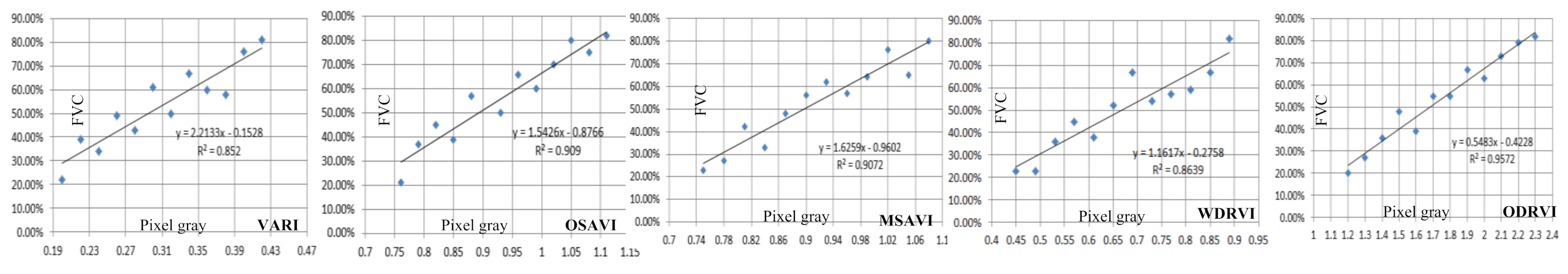
| Cities | OSAVI | WDRVI | MSAVI | VARI | ODRVI |
|---|---|---|---|---|---|
| Beijing | 0.418 | 0.447 | 0.414 | 0.255 | 0.866 |
| Hefei | 0.501 | 0.501 | 0.767 | 0.251 | 0.931 |
| Guangzhou | 0.597 | 0.559 | 0.866 | 0.226 | 0.998 |
| Sample Sites | Accuracy (%) | ||||
|---|---|---|---|---|---|
| ELF | LF | MF | MHF | HF | |
| Dashu Mountain Forest Park | 93.2 | 91.5 | 92.4 | 93.1 | 94.3 |
| Zepeng Mountain Forest Park | 92.7 | 92.3 | 92.8 | 93.3 | 94.1 |
| Parameters | ||||
|---|---|---|---|---|
| Winter: OLI 15 January 2016 | Spring: TM 30 May 2009 | Summer: ETM + 22 July 2012 | Autumn: OLI 11 October 2015 | |
| 2.13 | 2.29 | 2.57 | 2.38 | |
| 0.839 | 0.906 | 1.275 | 0.891 | |
| Year | Year | ||||
|---|---|---|---|---|---|
| 1999 | 0.465 | 1.67 | 2009 | 0.906 | 2.35 |
| 2000 | 0.681 | 2.36 | 2010 | 0.836 | 2.08 |
| 2001 | 0.411 | 1.88 | 2011 | 0.811 | 2.31 |
| 2002 | 1.297 | 2.63 | 2012 | 1.275 | 2.69 |
| 2003 | 0.763 | 2.29 | 2013 | 1.153 | 2.55 |
| 2004 | 0.823 | 2.41 | 2014 | 1.052 | 2.66 |
| 2005 | 1.057 | 2.56 | 2015 | 0.891 | 2.43 |
| 2006 | 1.103 | 2.59 | 2016 | 1.117 | 2.75 |
| 2007 | 0.947 | 2.51 | 2017 | 0.897 | 2.29 |
| 2008 | 0.864 | 2.28 | 2018 | 0.963 | 2.44 |
Publisher’s Note: MDPI stays neutral with regard to jurisdictional claims in published maps and institutional affiliations. |
© 2021 by the authors. Licensee MDPI, Basel, Switzerland. This article is an open access article distributed under the terms and conditions of the Creative Commons Attribution (CC BY) license (https://creativecommons.org/licenses/by/4.0/).
Share and Cite
Wang, Y.; Li, M. Annually Urban Fractional Vegetation Cover Dynamic Mapping in Hefei, China (1999–2018). Remote Sens. 2021, 13, 2126. https://doi.org/10.3390/rs13112126
Wang Y, Li M. Annually Urban Fractional Vegetation Cover Dynamic Mapping in Hefei, China (1999–2018). Remote Sensing. 2021; 13(11):2126. https://doi.org/10.3390/rs13112126
Chicago/Turabian StyleWang, Yuliang, and Mingshi Li. 2021. "Annually Urban Fractional Vegetation Cover Dynamic Mapping in Hefei, China (1999–2018)" Remote Sensing 13, no. 11: 2126. https://doi.org/10.3390/rs13112126
APA StyleWang, Y., & Li, M. (2021). Annually Urban Fractional Vegetation Cover Dynamic Mapping in Hefei, China (1999–2018). Remote Sensing, 13(11), 2126. https://doi.org/10.3390/rs13112126