Phytoplankton Biomass and the Hydrodynamic Regime in NEOM, Red Sea

Abstract

NEOM (short for Neo-Mustaqbal) is a $500 billion coastal city megaproject, currently under construction in the northwestern part of the Red Sea, off the coast of Tabuk province in Saudi Arabia, and its success will rely on the preservation of biodiverse marine ecosystems. Monitoring the variability of ecological indicators, such as phytoplankton, in relation to regional environmental conditions, is the foundation for such a goal. We provide a detailed description of the phytoplankton seasonal cycle of surface waters surrounding NEOM using satellite-derived chlorophyll-a (Chl-a) observations, based on a regionally-tuned product of the European Space Agency’s Ocean Colour Climate Change Initiative, at 1 km resolution, from 1997 to 2018. The analysis is also supported with in situ cruise datasets and outputs of a state-of-the-art high-resolution hydrodynamic model. The open waters of NEOM follow the oligotrophic character of the Northern Red Sea (NRS), with a peak during late winter and a minimum during late summer. Coral reef-bound regions, such as Sindala and Sharma, are characterised by higher Chl-a concentrations that peak during late summer. Most of the open waters around NEOM are influenced by the general cyclonic circulation of the NRS and local circulation features, while shallow reef-bound regions are more isolated. Our analysis provides the first description of the phytoplankton seasonality and the oceanographic conditions in NEOM, which may support the development of a regional marine conservation strategy.

1. Introduction

The Red Sea is a large marine ecosystem (LME) that lies between the African and Asian continental shelves, covering a distance of 2250 km. It is of vast economic importance, providing food to coastal communities as well as being a global trade route for goods from the Asian market and hydrocarbons to the Western world [1,2]. The northern part of the Red Sea is connected to the Mediterranean Sea via the Suez Canal, whilst the southern part is naturally connected to the Indian Ocean (Gulf of Aden) through the shallow strait of Bab-el-Mandeb. The Red Sea is considered a biodiversity hotspot [3], and hosts over 16,000 km² of coral reef ecosystems [4]. The Red Sea is also one of the warmest and most saline LMEs in the world [5,6,7], and as a result, has developed unique eurythermal coral reef ecosystems in its northern regions [8,9].

The Red Sea, and especially the Northern Red Sea (NRS), is one of the fastest warming tropical marine ecosystems in the world [6,7,10,11]. An alarming increase in regional warming (including marine heatwaves) has also been recorded over the past decades in the NRS [9,12,13,14]. Consequently, considering that coral bleaching events have already been reported in other areas of the Red Sea [9,15,16], even the heat-tolerant coral refuge that is present in the NRS may be threatened if its bleaching threshold is reached [8,9,13]. The NRS phytoplankton seasonal cycle follows a typical tropical regime; a bloom occurs during winter when more nutrients become available, while heavy stratification during summer contributes to lower Chl-a concentrations [12,17,18,19,20]. Phytoplankton phenology (bloom timing) is an important ecological indicator, as it drives the feeding and reproduction strategies of native species, and is, therefore, vital for sustaining current levels of biodiversity [21,22].

NEOM, which is short for the Ancient Greek-Arabic term Neo-Mustaqbal (“new future”), is a $500 bn megaproject that aims to build a fully automated city, operating as an independent economic zone in the NRS (Figure 1). The project will cover an area of 26,500 km², along a 468 km coastline characterised by coral-rich islets and bays. The region also hosts mangroves in some bays, narrow channels, and inland faces of offshore islands [23], and their density appears to be steadily increasing in the absence of coastal development [24]. The success of NEOM will rely on the preservation of its marine biodiversity hot spots, which hold significant economic value [25,26,27,28] and ultimately translate into food security and societal support through fisheries, recreation, and tourism. However, a project of this scale may pose risks to the local environment if not planned and managed according to a thorough knowledge of the surrounding ecosystems. For instance, it is estimated that around 70% of Saudi Arabia’s drinking water demands are met by desalinated water [29], and NEOM will likely rely on desalination plants for freshwater. The process of desalination releases brine as a by-product and can produce harmful pollutants, such as chlorine and copper [30], and could potentially have detrimental impacts on shallow coastal areas. Another potential hazard for the ecosystems is eutrophication (excessive inflow of nutrients, i.e., from fertilisers, aquaculture and wastewaters), which has been linked to harmful algal blooms [31] and coral bleaching [32] in the NRS. Thus, monitoring and understanding changes in ecological indicators are needed in order to support decision-making during the project.

Ecological indicators are metrics that quantify ecosystem properties such as health, vigour or resilience, and allow ecosystem changes to be monitored [33]. There are numerous indicators based on species abundance and diversity [34,35,36], but their estimation can be difficult, time-consuming and costly [36]. Ideally, ecological indicators should be easily understood, quantified in standard units, have an immediate response to changes, measured at adequate frequencies and low costs, and applicable to many locations to allow comparisons [22,33,37]. Phytoplankton biomass and phenology are important ecological indicators that can be used to assess the state of marine ecosystems [33,38]. Since phytoplankton constitute the base of the marine food web [22,39], alterations to their seasonal cycles may impact the recruitment of higher trophic levels (including commercially important species) that are dependent on the temporal synchrony of food availability [40,41,42,43]—an effect known as the match–mismatch hypothesis [44]. Satellite remote sensing of ocean colour can be used as a proxy for estimating phytoplankton abundance in large areas, at adequate temporal frequencies that enable seasonal cycles to be described in detail [38].

Daily ocean colour observations have been available at ~1 km resolution since 1997 and enable large-scale analysis of the interannual and decadal variability of phytoplankton phenology [45]. Although studies have been conducted in the broader NRS, detailed information assessing the seasonal variability of ecological indicators (i.e., phytoplankton abundance and phenology) and environmental conditions (physical regime) in the NEOM region are limited.

The goal of this study is to provide a comprehensive description of the satellite-derived phytoplankton seasonal cycle for the NRS waters surrounding NEOM, in relation to the physicochemical regime based on in situ datasets and outputs of a state-of-the-art hydrodynamic model. This multi-disciplinary approach aims to create a solid baseline for all future research on NEOM’s aquatic environment, and will ultimately be a useful tool for conservation managers to support their efforts to minimise detrimental impacts on the regional environment.

2. Materials and Methods

2.1. Satellite Remote Sensing Data and Study Area

Version 3.1 of the European Space Agency’s Ocean Colour Climate Change Initiative (ESA OC-CCI) was used in this study with additional data processing through the United Kingdom Natural Environment Research Council—Earth Observation Data Acquisition and Analysis Service (NEODAAS). This product consists of merged and bias-corrected Chl-a data from the Sea-Viewing Wide Field-of-View Sensor (SeaWiFS), Moderate Resolution Imaging Spectroradiometer (MODIS), Medium Resolution Imaging Spectrometer (MERIS) and Visible Infrared Imaging Radiometer Suite (VIIRS) satellite sensors [46]. The ESA OC-CCI is one of the most consistent, stable, and error-characterised time-series of global ocean-colour products based on several satellite sensors [47]. Level 3, mapped data were acquired at a 1 km spatial resolution, and a daily temporal resolution, for the period 1997–2018. The Chl-a data were averaged into monthly means to estimate the climatological phytoplankton biomass cycle. For seasonal analyses, quarterly periods were defined according to the seasonal variation in Chl-a concentrations (Winter: mid-December to mid-March, Spring: mid-March to mid-May, Summer: mid-May to mid-September, Autumn: mid-September to mid-December) [18]. To reduce estimation bias, pixels associated with shallow (<20 m) areas and/or coral reefs were removed.

The sea surrounding NEOM, similarly to the wider Red Sea, is optically complex, attributed to greater coloured dissolved organic matter absorption per unit Chl-a concentration [48]. As a result, standard algorithms systematically overestimate Chl-a when compared with in situ observations and region-specific algorithms may provide better results [49,50]. Therefore, our Chl-a dataset was regionally-tuned for the Red Sea by using the OC4-RG algorithm. This algorithm is based on the standard National Aeronautics and Space Administration (NASA) Ocean Colour 4 (OC4) algorithm, with a set of coefficients specifically tuned for the Red Sea (see Table 3 of Brewin et al. [51]). It performed significantly better (according to a point classification based on multiple statistical tests, see Figure 5 of Brewin et al. [51]) when compared with the standard NASA ocean colour algorithms, and other semi-analytical algorithms [51]. To our knowledge, this dataset comprises the highest quality satellite Chl-a product available in the study area.

Several areas of interest are presented in this study: the Gulf of Aqaba, Sindala, Sharma, the Port of Duba and the open sea of NEOM (Figure 1). These areas were chosen after visual analyses of monthly composite images, as well as their geographical and ecological importance. The Gulf of Aqaba has been a major shipping route for Israel (Eilat) and Jordan (Aqaba) for decades, and hosts popular diving destinations for tourists, due to the healthy coral reefs present there. Sindala is a shallow area situated in the western end of the NEOM region and is unique with regard to its extensive coral reefs and complex topography. In accordance with NEOM’s marine conservation project [52], Sindala (final name may differ) will be a designated nature reserve, due to its ecological importance. Sharma is a shallow lagoon enclosed by coral reefs and islets, located in the center of NEOM’s coastline. The Port of Duba is one of the most important ports in Northern Saudi Arabia due to its proximity to the Suez Canal. Unlike the aforementioned coastal areas, the port is surrounded by deeper waters (>100 m) and fewer coral reefs. Finally, the open sea is designated as the southwestern quarter of the NEOM region, where the depth is >200 m and is characterised by the absence of coral reefs. This open water region is a reference area that represents the broader biophysical conditions of the NRS.

A large part of NEOM’s coastal areas, especially the areas of interest in this study, are shallow (<30 m), optically complex waters (Figure 1). Remotely sensed Chl-a observations in such waters may have limitations due to suspended sediments, particulate matter, and/or dissolved organic matter, which does not covary in a predictable manner with Chl-a [53]. Scattering by sediments and underwater reflectance in shallow coastal waters (or coral reefs) may result in relatively high water-leaving radiance in the near-infrared wavelengths, which could overestimate the atmospheric correction [18]. Despite ESA OC-CCI using an optical water type approach to select amongst a number of chlorophyll algorithms [54], our observations in the shallow areas of interest may be influenced by the aforementioned factors, therefore, resulting in overestimated Chl-a concentrations [55]. However, high Chl-a values in shallow areas cannot be completely ignored, since these areas are covered by coral reefs that have been shown to enhance phytoplankton production [17,47,56,57]. In addition, Chl-a observations in areas with a similar shallow topography in the Red Sea have been validated with in situ measurements [47,57]. Higher resolution (300 m), regionally-tuned (OC4ME_RG algorithm, derived from the standard NASA OC4 algorithm, the MERIS ocean-colour sensor wavelength, and Red Sea regional tuning, as shown in Table 3 of Brewin et al. [51]) Chl-a datasets from Sentinel-3 Ocean and Land Colour Instrument (OLCI) were used to investigate whether our observations in such areas were trustworthy. These datasets were found to be in agreement with the ESA OC-CCI 1 km dataset for all areas of interest except Sindala (Figure S1). Therefore, the Sentinel-3 OLCI dataset was used to describe the seasonal cycle in Sindala, where deeper areas, with more accurate observations, were identifiable (Figure S2). The reason that the Sentinel-3 OLCI dataset was not used for every area is that it consists of only 4 years of observations (May 2016 to May 2020) in comparison to the 21 years of data that the ESA OC-CCI dataset provides. We note that the scope of this study is to assess the general phytoplankton seasonal variability in the sea surrounding NEOM, regardless of absolute concentrations.

2.2. Hydrodynamic Model

A high-resolution (1 km) state-of-the-art general circulation model (MITgcm [58]) was implemented for the Red Sea based on the latest available topographic data [59]. The model has 50 vertical, nonuniformly spaced vertical layers (z-coordinates), with an exponentially increasing thickness ranging from 4 m near the surface to 250 m in the deepest layer. There are a total of 18 layers in the first 150 m of depth. The simulation covers the period from January 2001 to December 2015 and was forced by a downscaled regional atmospheric product [60], with a spatial resolution of about 5 km. The model output has been shown to successfully describe the circulation dynamics, from the large-scale overturning circulation to the mesoscale vigorous eddy activity [12,59,61,62,63,64]. The current version of the model setup has been successfully validated against 469 independent CTD observations across the Red Sea, 76 independent CTD profiles available over the NEOM region, as well as satellite sea surface height and sea surface temperature data [59]. Daily data were averaged into the same quarterly periods as previously described for the Chl-a observations to create similar spatial plots and provide meaningful comparisons.

2.3. In Situ Data of Chl-a, Nutrients, Temperature and Salinity

In situ datasets were obtained from the first detailed oceanographic survey conducted in the NEOM region during 2017–2018 (R/V Dream Island). Three sampling cruises took place, during November 2017, February 2018 and April 2018. Seawater samples were acquired from four different depths (1, 20, 50 and 75 m) or from the surface (1 m) and near-bottom (1 m above max depth) if the depth was shallower than 20 m. Measurements were taken from multiple sampling stations across the NEOM region. Water samples were collected using NISKIN 5 L bottles. For determining Chl-a concentrations, 300 mL seawater samples were filtered on board using Whatman GF/F filters. The filters were kept in a dark, dry environment at approximately −20 °C. Chl-a concentration was subsequently determined in the Analytical Core Lab (ACL) of King Abdullah University of Science and Technology (KAUST) using a fluorometer according to an established protocol [65]. For the nutrient analysis, water samples were taken from the same water depths as for Chl-a, filtered through 0.45 μm membrane Millipore filters and collected in 100 mL polyethylene bottles, pretreated with 10% HCl. The samples were kept frozen (−20 °C) until their analysis in the KAUST ACL, using a nutrient autoanalyser following standard methods (e.g., for nitrite-nitrate [66]). Temperature and salinity were measured by means of a CTD probe (portable autographic instrument model SBE19 plus—data not shown) at multiple locations in the region and were used to further validate the hydrodynamic model outputs in this region.

In order to create seasonal vertical profiles for the open waters of NEOM, the in situ data from the deep sampling stations (>75 m) for the 3 cruises were plotted. The values of Chl-a and nitrate were averaged for each depth and month and then plotted vertically. All of the in situ Chl-a measurements were used to validate our satellite data (Figure S3) and support our area descriptions (seasonal cycles).

2.4. Sea Floor Morphology and Coral Reef Data

High-quality isobaths (isobath depths: 0, 1, 3, 10, 20, 50, 100, 200, 500, 1000 m) were provided by the Saudi Ports Authority and were linearly interpolated onto a grid, with a spatial resolution of 10 m, using a triangulation method in MATLAB R2019b. Coral reef locations were identified visually from nautical maps, habitat maps [67] and Google Earth satellite imagery. The outlines were created manually using Google Earth’s polygon tool (version 7.3) and were validated with the Global Distribution of Coral Reefs dataset (version 2018) produced by the UN Environment Programme—World Conservation Monitoring Centre (UNEP-WCMC). It should be noted that not all coral reefs can be captured with this method, as some potential coral reef locations (shallow areas, <30 m depth, in Figure 1) are not covered by the images. The purpose of highlighting coral reefs was to demonstrate the ecological importance and complexity of the region.

3. Results

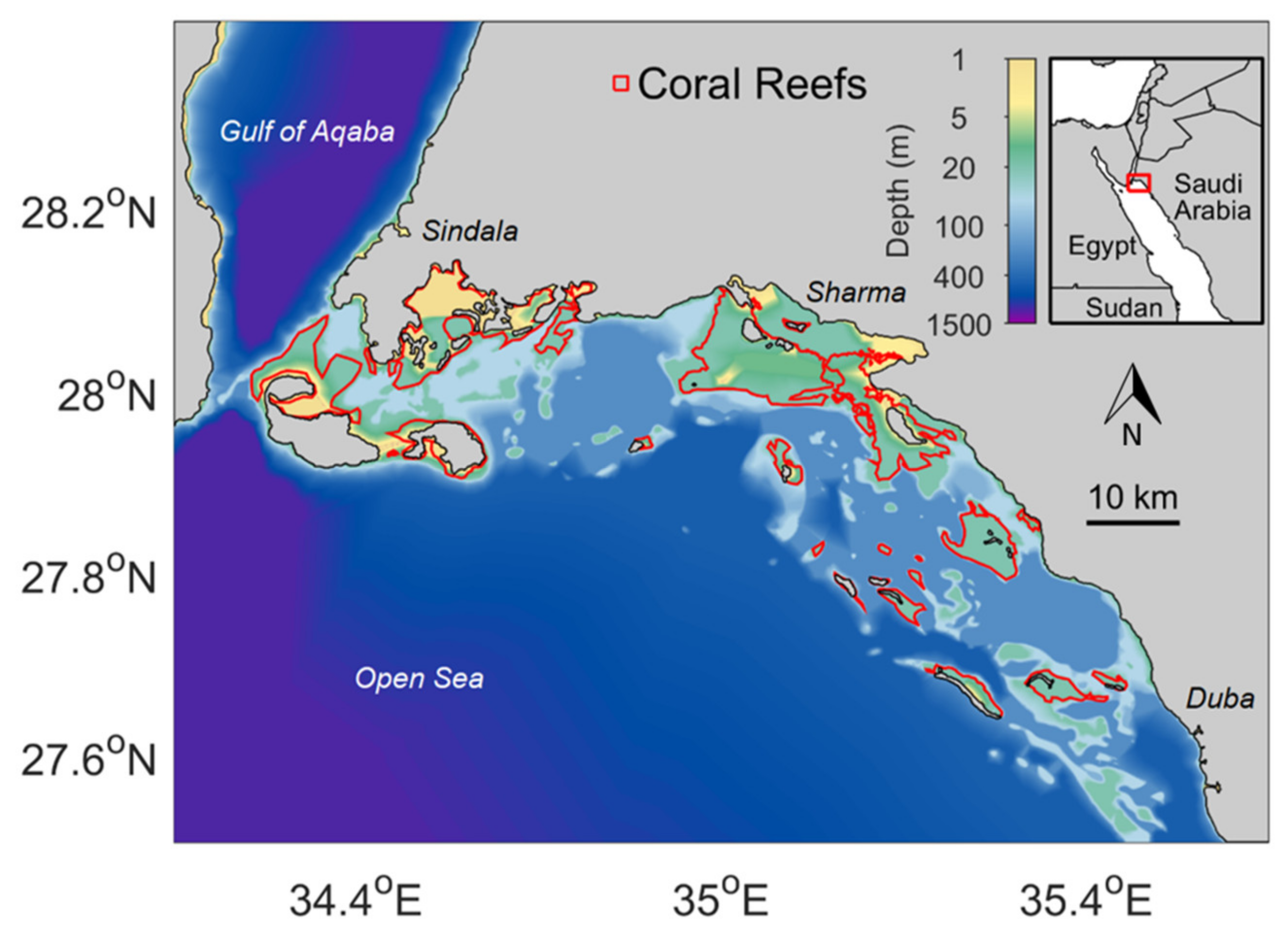
3.1. Area Description

The sea surrounding NEOM can be split into two main areas according to the bathymetry (Figure 1): shallow coastal waters and deeper open waters. The shallow coastal waters are characterised by coral reefs, shallow shelves and platforms that commonly extend up to 30 km towards the open sea. The northern part of this region (southern Gulf of Aqaba) is an exception since it lacks the large coral reef formations that are observed in the southern part, which are limited up until the Straits of Tiran. The shallow areas examined in this study (Sharma and Sindala) share a similar topography; vast areas covered by coral reefs. Sharma appears to have slightly deeper waters (~20 m) that are encircled by coral reefs, and thus can be classified as a coastal lagoon [68]. Sindala consists of smaller pools that are formed by coral reefs, making difficult its classification as a whole (Figure S2). The Port of Duba, although surrounded by large shallow areas, is directly connected to the open waters and reaches depths of 200 m in regions relatively close to the coast. Thus, the region can be considered as open water rather than coastal. The open waters in NEOM are characterised by a steep bottom slope, starting from the end of the shallow banks. Depths of more than 1000 m are observed in the central parts of the NRS and the Gulf of Aqaba. The Gulf of Aqaba is connected to the NRS through the Straits of Tiran, which consists of two main passages: the wider and deeper Enterprise Passage on the western end (sill depth ~260 m), and the narrower and shallower Grafton Passage closer to the island of Tiran (sill depth ~75 m). Another passage extends between the eastern side of Tiran and the coast of Saudi Arabia, through the coral reefs and banks, with a sill depth of ~16 m.

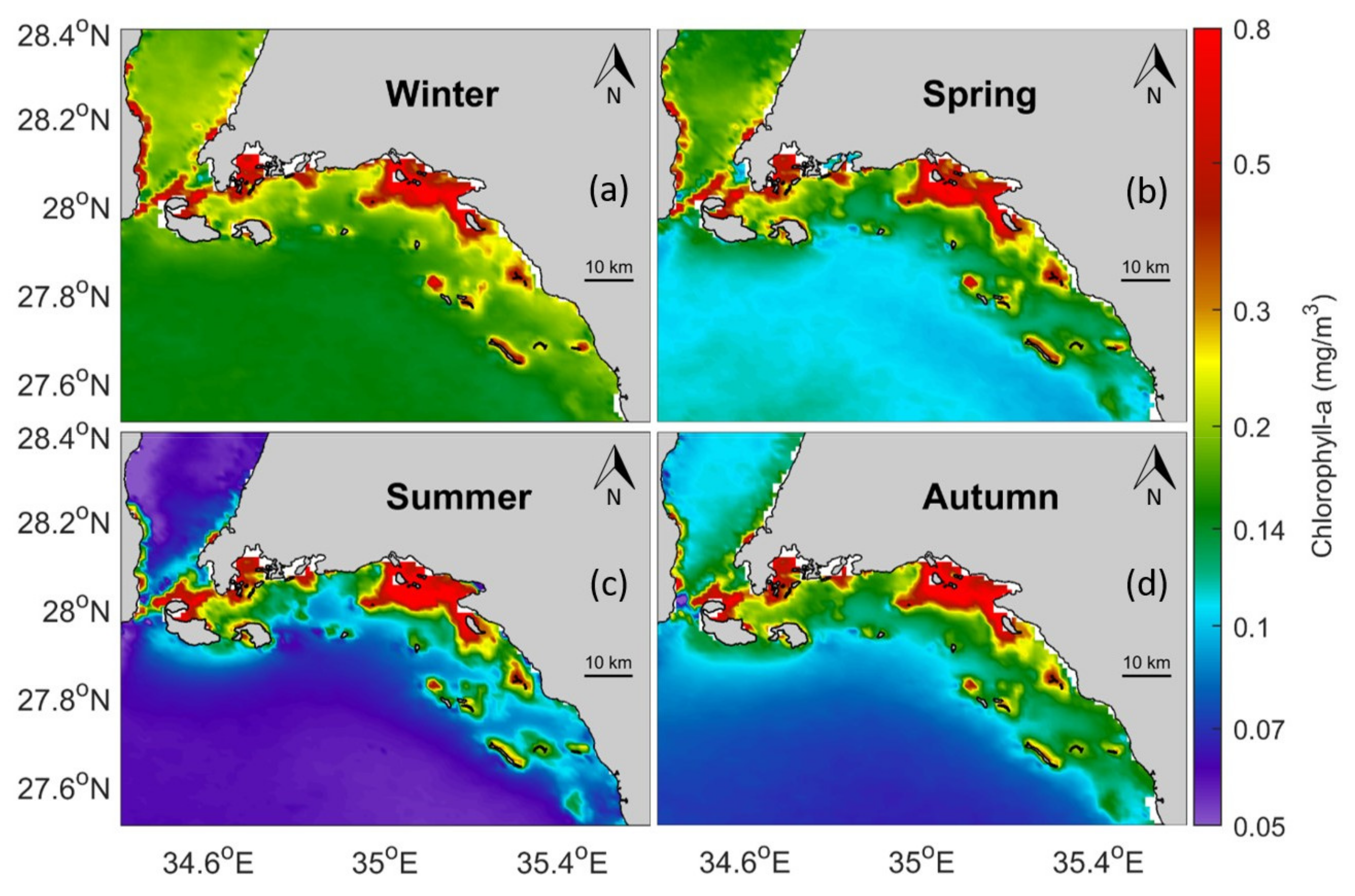
3.2. Remotely-Sensed Chl-a Observations

In this section, 21-years of Chl-a observations in the NEOM region are presented and their variability is analysed both spatially and temporally. The Chl-a seasonal climatology (Figure 2) splits the region into the same two main regions as the bathymetry. In general, the shallow coastal waters reveal consistently higher average Chl-a concentrations (e.g., 0.91 mg m⁻³ in Sharma and 0.52 mg m⁻³ in Sindala) than the open waters (0.11 mg m⁻³) throughout the year. The zone extending for up to 20 km between the coast and the open waters is characterised by Chl-a concentrations decreasing with distance from the coast. In the open waters, the main growth period of phytoplankton occurs during winter (Figure 2a), when average surface Chl-a concentrations exceed 0.15 mg m⁻³. In spring (Figure 2b), the Chl-a concentrations decline in the southern part of the NEOM region to 0.11 mg m⁻³, but remain relatively high in the Gulf of Aqaba (>0.19 mg m⁻³). During summer (Figure 2c), surface Chl-a concentrations drop to <0.07 mg m⁻³, and begin to increase again in autumn (Figure 2d) reaching 0.09 mg m⁻³ in the southern part and >0.1 mg m⁻³ in the Gulf of Aqaba.

The seasonal climatologies of surface Chl-a concentration in several areas of NEOM are presented in Figure 3. The open sea in NEOM (Figure 3b) is characterised by a peak in Chl-a during winter (February: 0.16 mg m⁻³), and a decrease in late summer (August: 0.06 mg m⁻³). Similarly, but with a larger seasonal difference than the open sea, Chl-a concentrations in the Gulf of Aqaba (Figure 3c) peak in winter, reaching 0.22 mg m⁻³ in February, while the lowest concentrations are observed in August (0.05 mg m⁻³. In Sindala (Figure 3e), the highest Chl-a concentrations occur during the summer, between July and September (0.58 mg m⁻³), and subsequently decline until February when the lowest values are observed (0.43 mg m⁻³). After February, Chl-a increases steadily until summer, with a transitional phase in spring (April-May) that completes this unique seasonal Chl-a cycle. Sharma (Figure 3f) is characterised by a similar Chl-a seasonal cycle, peaking in September (1.2 mg m⁻³) and reaching minimum concentrations in early spring (March: 0.65 mg m⁻³). The Port of Duba (Figure 3d) has a similar seasonal Chl-a cycle to the open sea, although is characterised by slightly higher Chl-a concentrations. Maximum Chl-a values of 0.18 mg m⁻³ occur in February, whilst minimum values (0.09 mg m⁻³) are reached in August.

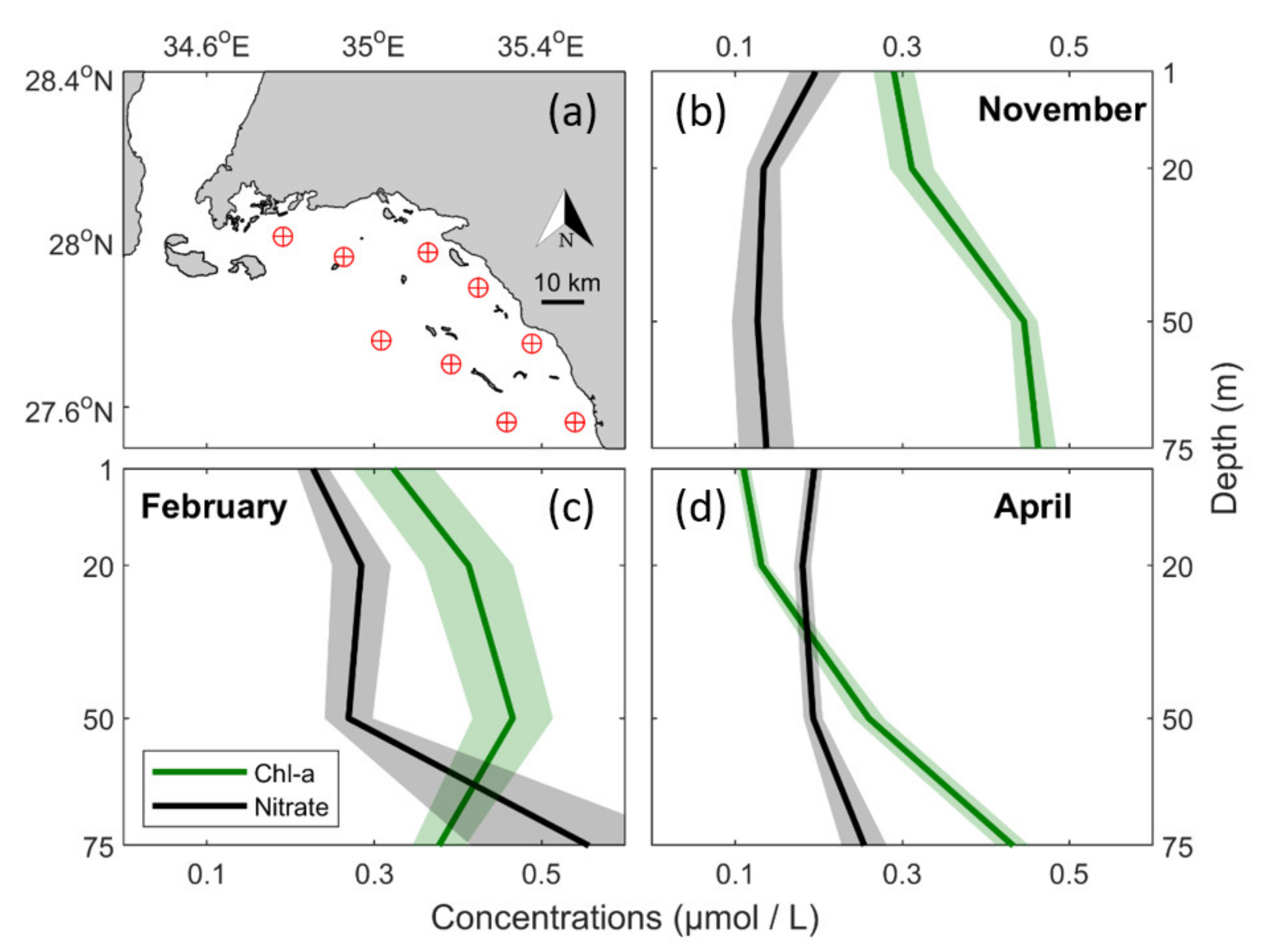
3.3. In Situ Observations

Monthly-averaged vertical profiles of Chl-a and nitrate concentration are presented for November 2017, February 2018 and April 2018 (Figure 4). In November (Figure 4b), higher Chl-a concentrations (bloom initiation) can be observed throughout the water column (0.30–0.48 mg m⁻³, from surface to 75 m depth), co-occurring with low nitrate concentrations (0.20 μmol L⁻¹ at the surface layer, and 0.12 μmol L⁻¹ from 20 m until 75 m depth). In February (Figure 4c), Chl-a concentrations remain equally high (main growing season) gradually increasing until 50 m depth (from 0.30 to 0.45 mg m⁻³), and then decline (0.37 mg m⁻³). Nitrate levels increase with depth starting from 0.24 μmol L⁻¹ at the surface and reach a maximum of 0.53 μmol L⁻¹ at 75 m. In April (Figure 4d), Chl-a concentrations are low at the surface (0.1 mg m⁻³) and increase with depth (up to 0.42 mg m⁻³), while nitrate concentrations remain relatively stable in the water column (between 0.22 and 0.26 μmol L⁻¹).

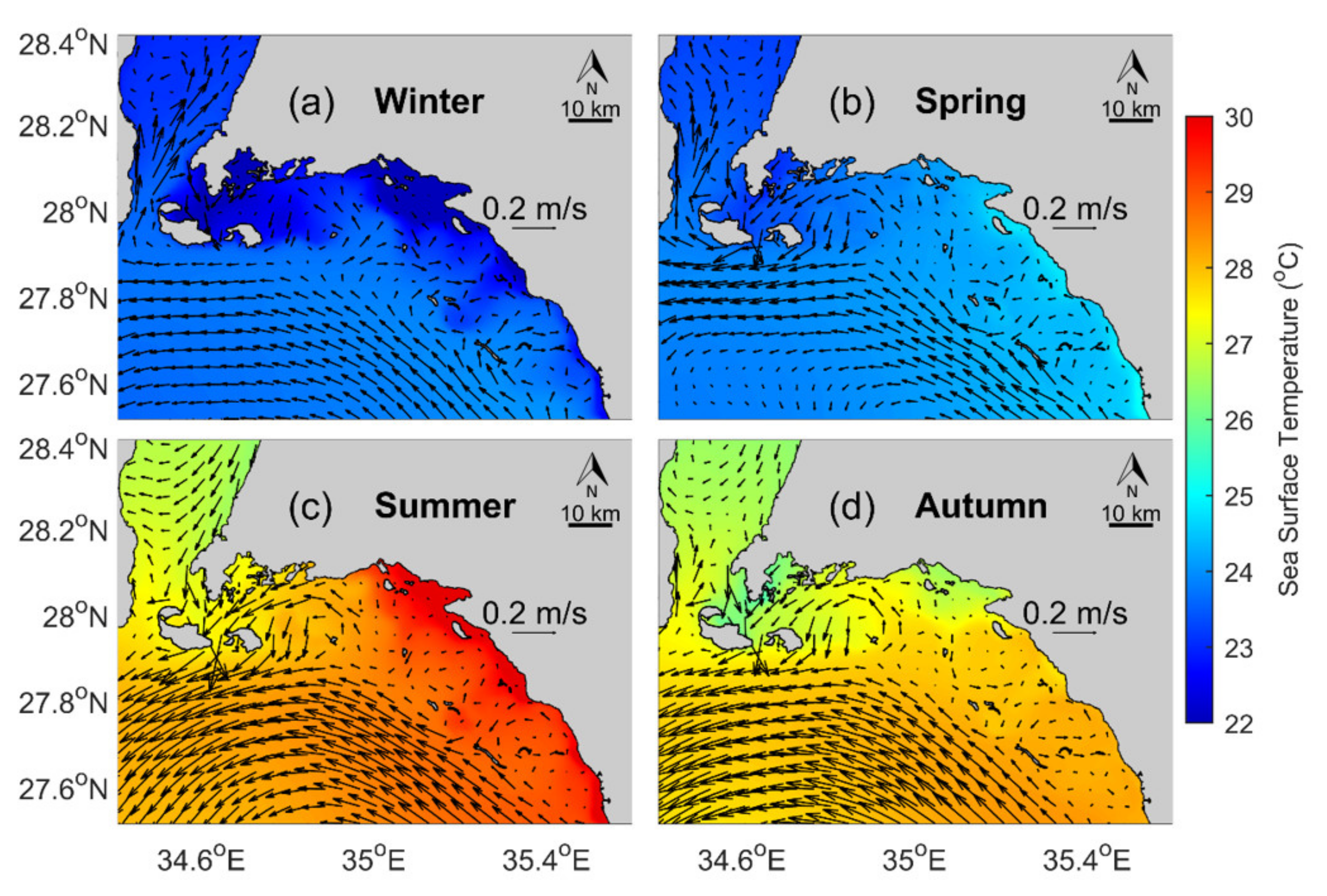
3.4. Oceanographic Setting

Several observations can be made from the climatological values derived from the physical outputs of the hydrodynamic model (Figure 5). Sea Surface Temperature (SST) in the open sea varies on average from 23 °C (winter) to 29 °C (summer), with increasing temperatures (decreasing in winter) apparent closer to the coast, especially inside the lagoons. Permanent northwestern surface currents flow in the open sea and become stronger in winter, creating small eddies at the shallow regions near the coasts. Average SST in the Gulf of Aqaba has a range of 22.5–27 °C. At the Straits of Tiran, the surface flow is towards the north during all seasons except for summer, when the average water transport shifts towards the south. In Sindala, the average SST varies from 22 to 27.5 °C, and a cyclonic eddy located just south of the area persists during all seasons. Sharma has an average SST range of 22 to 30 °C, while the average water transport is very low both inside and outside the lagoon. On average, SST at the Port of Duba varies from 23 to 29.5 °C and appears to be slightly lower near the coast in winter but slightly higher during the other seasons. The mean water transport near the coast is very low while the adjacent open waters follow the general open sea pattern of northwestern currents.

4. Discussion

The seasonal and spatial variability of phytoplankton biomass is examined for the first time in the NEOM region and is supported by in situ observations and a description of the oceanographic setting, based on a high-resolution regional model simulation. Distinct differences in the seasonality of Chl-a concentration can be observed between the separate study regions. Shallow coastal areas and lagoons, such as Sharma and Sindala, experience higher surface Chl-a concentrations in comparison to the open sea, the Gulf of Aqaba and the Port of Duba. The Chl-a seasonal cycle in the Port of Duba and the Gulf of Aqaba is similar to the NRS open waters, whereas significant differences in the seasonality and overall abundance of phytoplankton are observed in Sharma and Sindala.

The main phytoplankton growth period in the open waters of NEOM, including the Gulf of Aqaba and the Port of Duba, begins in autumn (early November) and lasts until spring (late April), resembling the distinct seasonality that has been previously observed over the broader NRS [12,18,20,47]. Average surface Chl-a concentrations remain low throughout the year, compared to other nearby environments such as the southern Red Sea, the Gulf of Aden or the Arabian Gulf [18,69,70,71]. Chl-a values in the Port of Duba are slightly higher than the open sea, which coincides with the fact that productivity and phytoplankton biomass in the Red Sea increases with proximity to the coast and the coral reefs [17,56,72]. The Gulf of Aqaba appears to reach slightly higher values during the winter peak and slightly lower values during summer, compared to the open waters of the NRS. Although our study area covers only the southern part of the Gulf of Aqaba, its seasonal cycle is in agreement with previous studies that reported a peak during late winter or early spring [72,73,74,75].

The in situ Chl-a measurements currently available from the NEOM region (Figure 4) are in agreement with the satellite-derived Chl-a seasonal cycle (Figure 3); higher surface (1 and 20 m—Figure 4) Chl-a concentrations occur during November and February, whilst concentrations are lower in April. The bloom initiation in November, the peak of the main phytoplankton growth period in February and the bloom termination in April can also be identified from these measurements. In November, higher Chl-a concentrations (bloom initiation) and lower nitrate concentrations are observed, as a result of their consumption by phytoplankton. There is also an increase in Chl-a concentration at 50 and 75 m, which indicates sufficient light penetration at those depths despite the high surface Chl-a concentration. In February, Chl-a concentrations remain high (bloom peak) and gradually increase until 50 m and then decline. The abrupt increase in nitrate at 75 m in February (Figure 4c), probably indicates limited light penetration for phytoplankton to utilise all of the nutrients available at that depth. In April, waters begin to stratify as SST increases and nutrients become limited in the surface layer [32]. Consequently, surface Chl-a concentrations are lower than in the other seasons but increase with depth, suggesting the presence of a subsurface chlorophyll maxima, which is common in tropical seas where nutrients are limiting primary production [18,20,76]. Since we were limited to a depth of 75 m in this study, we cannot estimate the exact depth of the subsurface chlorophyll maxima in April, nor ascertain their existence during November. Additional in situ sampling is required in the region in order to identify these features and to further validate our remotely-sensed observations.

Sharma and Sindala are distinct cases in our study region since their seasonal Chl-a cycles differ substantially from the general picture of the NRS (Figure 3) [12,17,18,20]. Their seasonal cycles appear to exhibit opposite patterns to those of the NEOM open waters. During summer, when the open waters in the region appear to be low in nutrients, the shallow coastal areas have access to nutrients, as indicated by the Chl-a concentrations. Although the underlying mechanism of this enhanced nutrient availability is not understood yet, it drives a Chl-a peak in late August and September. Chl-a concentrations in the coastal lagoons, Sharma and Sindala, are found to be higher than those in the open waters, possibly as a result of higher nutrient concentrations associated with the presence of coral reefs [17,56]. With depths <30 m, the absolute values observed within the lagoons are prone to bias, although the overall seasonality is stable and consistently observed every year. This unique seasonality may be a characteristic shared among the coastal lagoons of the Red Sea [47], since high Chl-a values have been previously observed in Al Wajh, Saudi Arabia, a region in the Central Red Sea with similar topography, during summer [77].

Consistent with most tropical mid-latitude marine environments, phytoplankton biomass in the Red Sea is limited by nutrient availability [17,18,51,72,78]. SST and mean water transport can provide insights on the processes that affect nutrient availability in the Red Sea, such as vertical mixing [12,20,32] and upwelling/downwelling [79]. Several observations can be made regarding the spatiotemporal variability of surface Chl-a concentrations in the NEOM region with regards to its oceanographic conditions, as described by the outputs of an extensively validated model of the general circulation of the Red Sea.

Surface Chl-a in the open waters of NEOM follows the seasonal succession previously reported in the NRS, where the highest concentrations occur during winter [12,18]. Since there is no significant runoff in the area, these winter blooms can be predominantly attributed to vertical mixing, as the deepening of the mixed layer redistributes nutrients in the water column [80]. When SST becomes lower, surface waters sink and are replaced by deep nutrient-rich waters, whilst strong stratification during summer prevents nutrients from reaching the surface, leading to the isolation of the deeper layer and the accumulation of organic material and nutrients in the near-bottom waters [12,17,18,19,20,32,47,75]. As previously mentioned, surface Chl-a concentrations in the Gulf of Aqaba remain higher than in the open waters of the NRS during winter. Both regions receive nutrients from mixing with deeper waters that take place mainly during winter. Mixed layers in the Gulf of Aqaba are generally deeper than the NRS, thus strong mixing may sustain higher nutrient availability [59,81]. The open waters in the Gulf of Aqaba and the NRS exhibit lower concentrations during summer, due to increased stratification, especially in the Gulf where Chl-a concentrations are even lower than in the NRS. This coincides with a change in direction of the average surface water transport from northward (entering the Gulf during winter), to southward (exiting the Gulf during the summer) (Figure 5). It is likely that the combination of increased stratification [12,17,18,19,20,32,47] and lack of surface inflow through the Straits of Tiran possibly causes this drop in surface Chl-a in the Gulf of Aqaba.

The permanent northwestern surface circulation in the open sea, which intensifies during winter, drives northward currents that flow near the coast and have been described previously as the Eastern Boundary Current [79,82]. This current affects all coastal regions (excluding lagoons) and thus they generally show common characteristics in terms of their physical properties, nutrient concentrations and seasonal variability. For example, the seasonality of Chl-a in the Port of Duba is very similar to the open sea. The boundary current [62,79,82] also creates several small eddies and bifurcating currents along natural barriers in the shallow regions near the coasts. Among them, a cyclonic eddy persists during all seasons to the south of Sindala (Figure 5) and could be a source of colder waters and nutrients for the region via upwelling. As highlighted in [57], such eddies may also enable the horizontal transfer of nutrients between different coral reef systems [17], contributing to higher Chl-a concentrations. Evidence of increased phytoplankton biomass can be detected many kilometers offshore of the coral reefs surrounding Sindala, where surface Chl-a concentrations are considerably higher than in the open sea (Figure 2).

As the seasonal Chl-a cycle in Sindala displays an opposite trend to that of the open sea, it is probable that the pools within Sindala (Figure S2) are enclosed with lower water exchange with the open sea. Additionally, due to the shallow bathymetry of the area, it is expected that the SST would be more susceptible to atmospheric forcing [83], with faster cooling (heating) occurring in the winter (summer). However, this is not the case here, as Sindala remains ~1 °C cooler on average during summer (Figure 5c) in comparison to the open sea. Furthermore, in situ measurements of temperature taken in November suggest that Sindala is indeed colder than every other area examined in marine areas of NEOM, including Sharma (Table S1).

Sharma is characterised by weak currents and appears to experience weaker water circulation than the other areas due to natural barriers. As a result, SST within the lagoon is driven mostly by atmospheric forcing, and changes rapidly, reaching temperatures >30 °C in the summer and <20 °C during winter. The mechanism behind the notably higher Chl-a concentrations in Sharma, combined with its unique seasonal cycle, cannot be fully described with the currently available data. High evaporation rates during summer may lead to water inflow from the open sea, which in turn, could provide nutrients and result in higher Chl-a concentrations in comparison to winter. Coastal lagoons rarely feature opposite Chl-a seasonal cycles to the surrounding open waters, making both Sharma and Sindala unique cases that require further investigation. Targeted in situ observations throughout the year are needed inside these lagoons to confirm our results, and to describe further the mechanism(s) driving these phenomena.

5. Conclusions

The synergistic use of satellite-derived Chl-a observations, high-resolution hydrodynamic model outputs and in situ datasets, facilitates the description of the seasonal and spatial patterns of phytoplankton, in relation to the oceanographic setting of the NEOM region, for the first time. Open waters in the region (including the Gulf of Aqaba and the Port of Duba sea area) are classified as oligotrophic and their conditions follow a similar pattern to what has been previously reported in the NRS. A distinct phytoplankton bloom occurs during winter, peaking in February, while minimum concentrations are observed during summer, especially in August. A northward-flowing boundary current is present throughout the year, creating smaller eddies near the coasts. Nutrient concentrations increase during winter as cooler surface waters sink and mix with nutrient-rich deep waters via convection.

The coastal lagoons examined (Sindala and Sharma) are unique, since their physical characteristics show an opposite surface Chl-a seasonal cycle (summer bloom) compared to the open waters, demonstrating the importance of localised studies in order to describe them more accurately. These lagoons should be the focal point of future ecological studies in the NEOM region, since they depict opposite seasonal trends to the previous reports on the open waters of the NRS, and may be indispensable in preserving the region’s biodiversity. Our first observation of this phenomenon is a significant step towards understanding its ecological importance.

There are many factors, such as sewage disposal, desalination pollutants, solid waste (e.g., plastic pollution), construction of infrastructure and dredging that could potentially disrupt the ecological balance in the vulnerable areas of NEOM (Sharma and Sindala). Therefore, the need for well-planned management from an ecological perspective is very important at the early stages of the megaproject. Stakeholders are aware of the importance of NEOM’s marine ecosystems and are planning to minimise potential damage during the construction phases, as well as any environmental impacts from the city’s operation. In this study, we provide a baseline for further research in the region, which can ultimately support conservation efforts, by providing clear and useful information for planning and decision-making.

Several recommendations can be made based on the results of this study, which may help to preserve one of the most important natural resources of the area, its marine biodiversity. Preserving healthy habitats and restoring any damaged ones should be a priority in NEOM, which in turn could become a vital economic asset for the region. The NEOM megaproject is a rare opportunity to demonstrate effective sustainable development and inspire future projects to follow similar environmentally responsible strategies.

Recommendations to NEOM Stakeholders

The natural characteristics and the restriction in the water exchange with the open sea are prohibitive factors for any large construction projects (such as ports and/or desalination plants) in both Sharma and Sindala. New infrastructures may alter the physical characteristics of these lagoons, which dictate their ecosystem functioning. Consequently, any disturbance can jeopardize the ecological balance (stable Chl-a seasonality) that currently exists, which may be vital in the preservation of the wider area’s biodiversity.

Anthropogenic pressure (i.e., waste from large hotels, golf courses, agriculture or aquaculture) in the coastal zone between the two lagoons (Sharma and Sindala), which is about 20 km long, should be kept to a minimum and within the marine conservation guidelines set by NEOM. This is because the water advection is always (all year round) towards Sindala and could potentially increase the levels of eutrophying pollutants (i.e., from sewage or fertilisers/pesticides) in the area. An excessive inflow of nutrients into an oligotrophic environment such as the NRS could have substantial impacts on marine biodiversity.

The coastline of the Gulf of Aqaba should be preferred instead of the coral-dense areas for any additional sea routes, ports and other infrastructures if needed. The combination of deep waters and steady surface water advection, predominantly towards the north, make it more resilient to any potential pollutants from anthropogenic activities that might otherwise end up in the vulnerable coral reefs of the NRS.

Clearly marked shipping routes should be enforced in the marine areas of NEOM, based on our best knowledge of the area’s ecology, such as the maps provided in this study. This would exclude traffic near the pristine coral reefs, and minimise potential sources of disturbance to aquatic organisms (i.e., underwater noise and anchor damage) that may alter the biodiversity balance.

References

1. Gladstone, W.; Tawfiq, N.; Nasr, D.; Andersen, I.; Cheung, C.; Drammeh, H.; Krupp, F.; Lintner, S. Sustainable use of renewable resources and conservation in the Red Sea and Gulf of Aden: Issues, needs and strategic actions. Ocean Coast. Manag. 1999, 42, 671–697. [Google Scholar] [CrossRef]
2. Gerges, M.A. The red sea and gulf of aden action plan—Facing the challenges of an ocean gateway. Ocean Coast. Manag. 2002, 45, 885–903. [Google Scholar] [CrossRef]
3. Hughes, T.P.; Bellwood, D.R.; Connolly, S.R. Biodiversity hotspots, centres of endemicity, and the conservation of coral reefs. Ecol. Lett. 2002, 5, 775–784. [Google Scholar] [CrossRef]
4. Roberts, C.M. Marine Biodiversity hotspots and conservation priorities for tropical reefs. Science 2002, 295, 1280–1284. [Google Scholar] [CrossRef] [Green Version]
5. Belkin, I.M. Rapid warming of Large Marine Ecosystems. Prog. Oceanogr. 2009, 81, 207–213. [Google Scholar] [CrossRef]
6. Raitsos, D.E.; Hoteit, I.; Prihartato, P.K.; Chronis, T.; Triantafyllou, G.; Abualnaja, Y. Abrupt warming of the Red Sea. Geophys. Res. Lett. 2011, 38. [Google Scholar] [CrossRef] [Green Version]
7. Carvalho, S.; Kürten, B.; Krokos, G.; Hoteit, I.; Ellis, J. The Red Sea. In World Seas: An Environmental Evaluation; Elsevier: Amsterdam, The Netherlands, 2019; pp. 49–74. [Google Scholar]
8. Fine, M.; Gildor, H.; Genin, A. A coral reef refuge in the Red Sea. Glob. Chang. Biol. 2013, 19, 3640–3647. [Google Scholar] [CrossRef] [PubMed]
9. Osman, E.O.; Smith, D.J.; Ziegler, M.; Kürten, B.; Conrad, C.; El-Haddad, K.M.; Voolstra, C.R.; Suggett, D.J. Thermal refugia against coral bleaching throughout the northern Red Sea. Glob. Chang. Biol. 2018, 24, e474–e484. [Google Scholar] [CrossRef]
10. Chaidez, V.; Dreano, D.; Agusti, S.; Duarte, C.M.; Hoteit, I. Decadal trends in Red Sea maximum surface temperature. Sci. Rep. 2017, 7, 8144. [Google Scholar] [CrossRef] [Green Version]
11. Krokos, G.; Papadopoulos, V.P.; Sofianos, S.; Hoteit, I. Assessing the long-term SST response of the Red Sea to natural climate variability. In Proceedings of the 2018 Ocean Sciences Meeting, Portland, OR, USA, 11–16 February 2018. [Google Scholar]
12. Gittings, J.A.; Raitsos, D.E.; Krokos, G.; Hoteit, I. Impacts of warming on phytoplankton abundance and phenology in a typical tropical marine ecosystem. Sci. Rep. 2018, 8. [Google Scholar] [CrossRef]
13. Genevier, L.G.C.; Jamil, T.; Raitsos, D.E.; Krokos, G.; Hoteit, I. Marine heatwaves reveal coral reef zones susceptible to bleaching in the Red Sea. Glob. Chang. Biol. 2019, 25, 2338–2351. [Google Scholar] [CrossRef] [PubMed] [Green Version]
14. Krokos, G.; Papadopoulos, V.P.; Sofianos, S.S.; Ombao, H.; Dybczak, P.; Hoteit, I. Natural Climate Oscillations may Counteract Red Sea Warming Over the Coming Decades. Geophys. Res. Lett. 2019, 46, 3454–3461. [Google Scholar] [CrossRef] [Green Version]
15. Furby, K.A.; Bouwmeester, J.; Berumen, M.L. Susceptibility of central Red Sea corals during a major bleaching event. Coral Reefs 2013, 32, 505–513. [Google Scholar] [CrossRef]
16. Pineda, J.; Starczak, V.; Tarrant, A.; Blythe, J.; Davis, K.; Farrar, T.; Berumen, M.; Da Silva, J.C.B. Two spatial scales in a bleaching event: Corals from the mildest and the most extreme thermal environments escape mortality. Limnol. Oceanogr. 2013, 58, 1531–1545. [Google Scholar] [CrossRef] [Green Version]
17. Acker, J.; Leptoukh, G.; Shen, S.; Zhu, T.; Kempler, S. Remotely-sensed chlorophyll a observations of the northern Red Sea indicate seasonal variability and influence of coastal reefs. J. Mar. Syst. 2008, 69, 191–204. [Google Scholar] [CrossRef]
18. Raitsos, D.E.; Pradhan, Y.; Brewin, R.J.W.; Stenchikov, G.; Hoteit, I. Remote sensing the phytoplankton seasonal succession of the Red Sea. PLoS ONE 2013, 8, e64909. [Google Scholar] [CrossRef] [PubMed] [Green Version]
19. Raitsos, D.E.; Yi, X.; Platt, T.; Racault, M.F.; Brewin, R.J.W.; Pradhan, Y.; Papadopoulos, V.P.; Sathyendranath, S.; Hoteit, I. Monsoon oscillations regulate fertility of the Red Sea. Geophys. Res. Lett. 2015, 42, 855–862. [Google Scholar] [CrossRef] [Green Version]
20. Gittings, J.A.; Raitsos, D.E.; Kheireddine, M.; Racault, M.-F.; Claustre, H.; Hoteit, I. Evaluating tropical phytoplankton phenology metrics using contemporary tools. Sci. Rep. 2019, 9. [Google Scholar] [CrossRef]
21. Kosobokova, K.N. The reproductive cycle and life history of the Arctic copepod Calanus glacialis in the White Sea. Polar Biol. 1999, 22, 254–263. [Google Scholar] [CrossRef]
22. Hays, G.; Richardson, A.; Robinson, C. Climate change and marine plankton. Trends Ecol. Evol. 2005, 20, 337–344. [Google Scholar] [CrossRef] [PubMed]
23. Kumar, A.; Khan, M.A.; Muqtadir, A. Distribution of mangroves along the Red Sea coast of the Arabian Peninsula: Part-I: The northern coast of western Saudi Arabia. Earth Sci. India 2010, 3, 28–42. [Google Scholar]
24. Almahasheer, H.; Aljowair, A.; Duarte, C.M.; Irigoien, X. Decadal stability of Red Sea mangroves. Estuar. Coast. Shelf Sci. 2016, 169, 164–172. [Google Scholar] [CrossRef] [Green Version]
25. Pearce, D.W. The value of biodiversity. Microb. Divers. Bioprospecting 2003, 469–475. [Google Scholar] [CrossRef]
26. Turpie, J.K.; Heydenrych, B.J.; Lamberth, S.J. Economic value of terrestrial and marine biodiversity in the Cape Floristic Region: Implications for defining effective and socially optimal conservation strategies. Biol. Conserv. 2003, 112, 233–251. [Google Scholar] [CrossRef]
27. Beaumont, N.J.; Austen, M.C.; Mangi, S.C.; Townsend, M. Economic valuation for the conservation of marine biodiversity. Mar. Pollut. Bull. 2008, 56, 386–396. [Google Scholar] [CrossRef]
28. Rees, S.E.; Rodwell, L.D.; Attrill, M.J.; Austen, M.C.; Mangi, S.C. The value of marine biodiversity to the leisure and recreation industry and its application to marine spatial planning. Mar. Policy 2010, 34, 868–875. [Google Scholar] [CrossRef]
29. Alsarhan, A.; Zatari, T.; Al-Asaly, M.; Mirza, K.; Harthi, A.; Othman, M.; Babiker, M.; Khan, A.; Aljabr, A.; Albuqami, F. Third National Communication of the Kingdom of Saudi Arabia; Designated National Authority (DNA) of Saudi Arabia: Riyadh, Saudi Arabia, 2016. [Google Scholar]
30. Hoepner, T.; Lattemann, S. Chemical impacts from seawater desalination plants—A case study of the northern Red Sea. Desalination 2003, 152, 133–140. [Google Scholar] [CrossRef]
31. Gokul, E.A.; Raitsos, D.E.; Gittings, J.A.; Hoteit, I. Developing an Atlas of harmful algal blooms in the Red Sea: Linkages to local aquaculture. Remote Sens. 2020, 12, 3695. [Google Scholar] [CrossRef]
32. Genin, A.; Lazar, B.; Brenner, S. Vertical mixing and coral death in the Red Sea following the eruption of Mount Pinatubo. Nature 1995, 377, 507–510. [Google Scholar] [CrossRef]
33. Platt, T.; Sathyendranath, S. Ecological indicators for the pelagic zone of the ocean from remote sensing. Remote Sens. Environ. 2008, 112, 3426–3436. [Google Scholar] [CrossRef]
34. Ludwig, J.A.; QUARTET, L.; Reynolds, J.F.; Reynolds, J. Statistical Ecology: A Primer in Methods and Computing; John Wiley & Sons: Hoboken, NJ, USA, 1988; Volume 1. [Google Scholar]
35. Legendre, P.; Legendre, L. Numerical Ecology; Elsevier: Amsterdam, The Netherlands, 2012. [Google Scholar]
36. Heink, U.; Kowarik, I. What criteria should be used to select biodiversity indicators? Biodivers. Conserv. 2010, 19, 3769–3797. [Google Scholar] [CrossRef]
37. McQuatters-Gollop, A.; Raitsos, D.E.; Edwards, M.; Pradhan, Y.; Mee, L.D.; Lavender, S.J.; Attrill, M.J. A long-term chlorophyll dataset reveals regime shift in North Sea phytoplankton biomass unconnected to nutrient levels. Limnol. Oceanogr. 2007, 52, 635–648. [Google Scholar] [CrossRef]
38. Racault, M.-F.; Platt, T.; Sathyendranath, S.; Irba, A.E.; Martinez Vicente, V.; Brewin, R.J.W. Plankton indicators and ocean observing systems: Support to the marine ecosystem state assessment. J. Plankton Res. 2014, 36, 621–629. [Google Scholar] [CrossRef] [Green Version]
39. Falkowski, P.G.; Raven, J.A. Aquatic Photosynthesis; Princeton University Press: Princeton, NJ, USA, 2013. [Google Scholar]
40. Beaugrand, G.; Brander, K.M.; Alistair Lindley, J.; Souissi, S.; Reid, P.C. Plankton effect on cod recruitment in the North Sea. Nature 2003, 426, 661–664. [Google Scholar] [CrossRef] [PubMed]
41. Edwards, M.; Richardson, A.J. Impact of climate change on marine pelagic phenology and trophic mismatch. Nature 2004, 430, 881–884. [Google Scholar] [CrossRef]
42. Platt, T.; Fuentes-Yaco, C.; Frank, K.T. Spring algal bloom and larval fish survival. Nature 2003, 423, 398–399. [Google Scholar] [CrossRef]
43. Koeller, P.; Fuentes-Yaco, C.; Platt, T.; Sathyendranath, S.; Richards, A.; Ouellet, P.; Orr, D.; Skuladottir, U.; Wieland, K.; Savard, L.; et al. Basin-scale coherence in phenology of shrimps and phytoplankton in the North Atlantic Ocean. Science 2009, 324, 791–793. [Google Scholar] [CrossRef]
44. Cushing, D.H. Plankton production and year-class strength in fish populations: An update of the match/mismatch hypothesis. Adv. Mar. Biol. 1990, 26, 249–293. [Google Scholar] [CrossRef]
45. Racault, M.-F.; Sathyendranath, S.; Brewin, R.J.W.; Raitsos, D.E.; Jackson, T.; Platt, T. Impact of El Niño Variability on Oceanic Phytoplankton. Front. Mar. Sci. 2017, 4. [Google Scholar] [CrossRef] [Green Version]
46. Sathyendranath, S.; Brewin, R.J.W.; Brockmann, C.; Brotas, V.; Calton, B.; Chuprin, A.; Cipollini, P.; Couto, A.; Dingle, J.; Doerffer, R.; et al. An Ocean-colour time series for use in climate studies: The Experience of the Ocean-Colour Climate Change Initiative (OC-CCI). Sensors 2019, 19, 4285. [Google Scholar] [CrossRef] [Green Version]
47. Racault, M.-F.; Raitsos, D.E.; Berumen, M.L.; Brewin, R.J.W.; Platt, T.; Sathyendranath, S.; Hoteit, I. Phytoplankton phenology indices in coral reef ecosystems: Application to ocean-color observations in the Red Sea. Remote Sens. Environ. 2015, 160, 222–234. [Google Scholar] [CrossRef] [Green Version]
48. Kheireddine, M.; Ouhssain, M.; Calleja, M.L.; Morán, X.A.G.; Sarma, Y.V.B.; Tiwari, S.P.; Jones, B.H. Characterization of light absorption by chromophoric dissolved organic matter (CDOM) in the upper layer of the Red Sea. Deep Sea Res. Part I Oceanogr. Res. Pap. 2018, 133, 72–84. [Google Scholar] [CrossRef] [Green Version]
49. Brewin, R.J.W.; Raitsos, D.E.; Pradhan, Y.; Hoteit, I. Comparison of chlorophyll in the Red Sea derived from MODIS-Aqua and in vivo fluorescence. Remote Sens. Environ. 2013, 136, 218–224. [Google Scholar] [CrossRef]
50. Brewin, R.J.W.; Morán, X.A.G.; Raitsos, D.E.; Gittings, J.A.; Calleja, M.L.; Viegas, M.; Ansari, M.I.; Al-Otaibi, N.; Huete-Stauffer, T.M.; Hoteit, I. Factors regulating the relationship between total and size-fractionated chlorophyll-a in coastal waters of the Red Sea. Front. Microbiol. 2019, 10. [Google Scholar] [CrossRef] [PubMed]
51. Brewin, R.J.W.; Raitsos, D.E.; Dall’Olmo, G.; Zarokanellos, N.; Jackson, T.; Racault, M.-F.; Boss, E.S.; Sathyendranath, S.; Jones, B.H.; Hoteit, I. Regional ocean-colour chlorophyll algorithms for the Red Sea. Remote Sens. Environ. 2015, 165, 64–85. [Google Scholar] [CrossRef] [Green Version]
52. Ameer, A.E. NEOM: Introducing a new era of sustainable development. In Proceedings of the Red Sea Research Center Open Science Conference, Thuwal, Saudi Arabia, 29–30 October 2019. [Google Scholar]
53. Sathyendranath, S. Remote Sensing of Ocean Colour in Coastal, and Other Optically-Complex, Waters; International Ocean Colour Coordinating Group (IOCCG): Dartmouth, NS, Canada, 2000. [Google Scholar]
54. Jackson, T.; Sathyendranath, S.; Mélin, F. An improved optical classification scheme for the Ocean Colour Essential Climate Variable and its applications. Remote Sens. Environ. 2017, 203, 152–161. [Google Scholar] [CrossRef]
55. Jacobs, Z.L.; Jebri, F.; Raitsos, D.E.; Popova, E.; Srokosz, M.; Painter, S.C.; Nencioli, F.; Roberts, M.; Kamau, J.; Palmer, M.; et al. Shelf-Break Upwelling and Productivity Over the North Kenya Banks: The Importance of Large-Scale Ocean Dynamics. J. Geophys. Res. Ocean. 2020, 125. [Google Scholar] [CrossRef] [Green Version]
56. Rasheed, M.; Badran, M.; Richter, C.; Huettel, M. Effect of reef framework and bottom sediment on nutrient enrichment in a coral reef of the Gulf of Aqaba, Red Sea. Mar. Ecol. Prog. Ser. 2002, 239, 277–285. [Google Scholar] [CrossRef]
57. Raitsos, D.E.; Brewin, R.J.W.; Zhan, P.; Dreano, D.; Pradhan, Y.; Nanninga, G.B.; Hoteit, I. Sensing coral reef connectivity pathways from space. Sci. Rep. 2017, 7. [Google Scholar] [CrossRef] [Green Version]
58. Marshall, J.; Adcroft, A.; Hill, C.; Perelman, L.; Heisey, C. A finite-volume, incompressible Navier Stokes model for studies of the ocean on parallel computers. J. Geophys. Res. Oceans 1997, 102, 5753–5766. [Google Scholar] [CrossRef] [Green Version]
59. Krokos, G.; Cerovecki, I.; Zhan, P.; Hoteit, I.; Hendershott, M.C. Processes controlling the seasonal evolution of Mixed Layers in the Red Sea. In Proceedings of the Ocean Sciences Meeting 2020, San Diego, CA, USA, 16–21 February 2020. [Google Scholar]
60. Viswanadhapalli, Y.; Dasari, H.P.; Langodan, S.; Challa, V.S.; Hoteit, I. Climatic features of the Red Sea from a regional assimilative model. Int. J. Clim. 2017, 37, 2563–2581. [Google Scholar] [CrossRef]
61. Yao, F.; Hoteit, I.; Pratt, L.J.; Bower, A.S.; Zhai, P.; Köhl, A.; Gopalakrishnan, G. Seasonal overturning circulation in the Red Sea: 1. Model validation and summer circulation. J. Geophys. Res. Ocean. 2014, 119, 2238–2262. [Google Scholar] [CrossRef] [Green Version]
62. Yao, F.; Hoteit, I.; Pratt, L.J.; Bower, A.S.; Köhl, A.; Gopalakrishnan, G.; Rivas, D. Seasonal overturning circulation in the Red Sea: 2. Winter circulation. J. Geophys. Res. Ocean. 2014, 119, 2263–2289. [Google Scholar] [CrossRef] [Green Version]
63. Zhan, P.; Subramanian, A.C.; Yao, F.; Hoteit, I. Eddies in the Red Sea: A statistical and dynamical study. J. Geophys. Res. Ocean. 2014, 119, 3909–3925. [Google Scholar] [CrossRef] [Green Version]
64. Zhan, P.; Krokos, G.; Guo, D.; Hoteit, I. Three-dimensional signature of the Red Sea Eddies and eddy-induced transport. Geophys. Res. Lett. 2019, 46, 2167–2177. [Google Scholar] [CrossRef] [Green Version]
65. Holm-Hansen, O.; Lorenzen, C.J.; Holmes, R.W.; Strickland, J.D.H. Fluorometric Determination of Chlorophyll. ICES J. Mar. Sci. 1965, 30, 3–15. [Google Scholar] [CrossRef]
66. Strickland, J.D.H.; Parsons, T.R. A Practical Handbook of Seawater Analysis; Fisheries Research Board of Canada: Ottawa, QC, Canada, 1972. [Google Scholar]
67. Bruckner, A.; Rowlands, G.; Riegl, B.; Purkis, S.J.; Williams, A.; Renaud, P. Khaled bin Sultan Living Oceans Foundation Atlas of Saudi Arabian Red Sea Marine Habitats; Panoramic Press: Phoenix, AZ, USA, 2013; p. 262. [Google Scholar]
68. Kjerfve, B. Coastal lagoons. In Elsevier Oceanography Series; Elsevier: Amsterdam, The Netherlands, 1994; Volume 60, pp. 1–8. [Google Scholar]
69. Dreano, D.; Raitsos, D.E.; Gittings, J.A.; Krokos, G.; Hoteit, I. The Gulf of Aden Intermediate Water Intrusion Regulates the Southern Red Sea Summer Phytoplankton Blooms. PLoS ONE 2016, 11, e0168440. [Google Scholar] [CrossRef] [Green Version]
70. Gittings, J.A.; Raitsos, D.E.; Racault, M.-F.; Brewin, R.J.W.; Pradhan, Y.; Sathyendranath, S.; Platt, T. Seasonal phytoplankton blooms in the Gulf of Aden revealed by remote sensing. Remote Sens. Env. 2017, 189, 56–66. [Google Scholar] [CrossRef] [Green Version]
71. Al-Naimi, N.; Raitsos, D.E.; Ben-Hamadou, R.; Soliman, Y. Evaluation of Satellite retrievals of chlorophyll-a in the Arabian Gulf. Remote Sens. 2017, 9, 301. [Google Scholar] [CrossRef] [Green Version]
72. Levanon-Spanier, I.; Padan, E.; Reiss, Z. Primary production in a desert-enclosed sea—The Gulf of Elat (Aqaba), Red Sea. Deep Sea Res. Part A Oceanogr. Res. Pap. 1979, 26, 673–685. [Google Scholar] [CrossRef]
73. Labiosa, R.G.; Arrigo, K.R.; Genin, A.; Monismith, S.G.; Van Dijken, G. The interplay between upwelling and deep convective mixing in determining the seasonal phytoplankton dynamics in the Gulf of Aqaba: Evidence from SeaWiFS and MODIS. Limnol. Oceanogr. 2003, 48, 2355–2368. [Google Scholar] [CrossRef] [Green Version]
74. Al-Najjar, T.; Badran, M.I.; Richter, C.; Meyerhoefer, M.; Sommer, U. Seasonal dynamics of phytoplankton in the Gulf of Aqaba, Red Sea. Hydrobiologia 2007, 579, 69–83. [Google Scholar] [CrossRef]
75. Tilstra, A.; Van Hoytema, N.; Cardini, U.; Bednarz, V.N.; Rix, L.; Naumann, M.S.; Al-Horani, F.A.; Wild, C. Effects of Water Column Mixing and Stratification on Planktonic Primary Production and Dinitrogen Fixation on a Northern Red Sea Coral Reef. Front. Microbiol. 2018, 9. [Google Scholar] [CrossRef]
76. Weikert, H. Plankton and the pelagic environment. Red Sea 1987, 90–111. [Google Scholar] [CrossRef]
77. Devassy, R.P.; El-Sherbiny, M.M.; Al-Sofyani, A.M.; Al-Aidaroos, A.M. Spatial variation in the phytoplankton standing stock and diversity in relation to the prevailing environmental conditions along the Saudi Arabian coast of the northern Red Sea. Mar. Biodivers. 2017, 47, 995–1008. [Google Scholar] [CrossRef]
78. Doney, S.C. Plankton in a warmer world. Nature 2006, 444, 695–696. [Google Scholar] [CrossRef] [PubMed] [Green Version]
79. Sofianos, S.S. An Oceanic General Circulation Model (OGCM) investigation of the Red Sea circulation: 2. Three-dimensional circulation in the Red Sea. J. Geophys. Res. 2003, 108. [Google Scholar] [CrossRef] [Green Version]
80. Polovina, J.J.; Mitchum, G.T.; Evans, G.T. Decadal and basin-scale variation in mixed layer depth and the impact on biological production in the Central and North Pacific, 1960–1988. Deep Sea Res. Part I Oceanogr. Res. Pap. 1995, 42, 1701–1716. [Google Scholar] [CrossRef]
81. Papadopoulos, V.P.; Zhan, P.; Sofianos, S.S.; Raitsos, D.E.; Qurban, M.; Abualnaja, Y.; Bower, A.; Kontoyiannis, H.; Pavlidou, A.; Asharaf, T.T.M.; et al. Factors governing the deep ventilation of the Red Sea. J. Geophys. Res. Ocean. 2015, 120, 7493–7505. [Google Scholar] [CrossRef] [Green Version]
82. Asfahani, K.; Krokos, G.; Papadopoulos, V.P.; Jones, B.H.; Sofianos, S.; Kheireddine, M.; Hoteit, I. Capturing a Mode of Intermediate Water Formation in the Red Sea. J. Geophys. Res. Ocean. 2020, 125, e2019JC015803. [Google Scholar] [CrossRef]
83. Moeller, C.C.; Huh, O.K.; Roberts, H.H.; Gumley, L.E.; Menzel, W.P. Response of Louisiana coastal environments to a cold front passage. J. Coast. Res. 1993, 9, 434–447. [Google Scholar]
Figure 1. Bathymetry of the Northern Red Sea surrounding NEOM. The areas examined in this paper, the Gulf of Aqaba, Sindala, Sharma, the Port of Duba and the open sea, are marked on the map. The red lines represent the peripheries of the main coral reef formations.
Remotesensing 13 02082 g001
Figure 2. Seasonal climatological maps (21 years) of satellite-derived Chlorophyll-a (mg/m3) over the NEOM region in the Northern Red Sea during: (a) Winter: mid-December to mid-March, (b) Spring: mid-March to mid-May, (c) Summer: mid-May to mid-September, (d) Autumn: mid-September to mid-December).
Remotesensing 13 02082 g002
Figure 3. Climatology of Chl-a in the NEOM region based on 21 years of satellite observations (1997–2018). In panel (a) the overall climatology of the region is plotted spatially along with the areas examined in this study. The bounding box for each area is also highlighted on the map. The seasonal climatology of Chl-a concentration (mg/m3) is presented for: (b) the open sea, (c) the Gulf of Aqaba, (d), the Port of Duba, (e) Sindala and (f) Sharma Bay. Note that the time-series plots for Sindala and Sharma have different y-axis scales, to account for the higher Chl-a concentrations observed there, and highlight their seasonal oscillations.
Remotesensing 13 02082 g003
Figure 4. In situ measurements of Chl-a and nitrate taken during three research cruises in the NEOM region in 2017–2018. The locations of the sampling stations are shown in panel (a). Vertical profiles for Chl-a and nitrate are presented during: (b) November, (c) February and (d) April. Samples were collected at depths of 1, 20, 50 and 75 m.
Remotesensing 13 02082 g004
Figure 5. Mean water circulation velocity and SST of the study area, calculated from a hydrodynamic model running through 1980–2018, for seasons: (a) Winter: mid-December to mid-March, (b) Spring: mid-March to mid-May, (c) Summer: mid-May to mid-September, (d) Autumn: mid-September to mid-December.
Remotesensing 13 02082 g005
Publisher’s Note: MDPI stays neutral with regard to jurisdictional claims in published maps and institutional affiliations.