Abstract
Digital terrain models (DTMs) are important for a variety of applications in geosciences as a valuable information source in forest management planning, forest inventory, hydrology, etc. Despite their value, a DTM in a forest area is typically lower quality due to inaccessibility and limited data sources that can be used in the forest environment. In this paper, we assessed the accuracy of close-range remote sensing techniques for DTM data collection. In total, four data sources were examined, i.e., handheld personal laser scanning (PLShh, GeoSLAM Horizon), terrestrial laser scanning (TLS, FARO S70), unmanned aerial vehicle (UAV) photogrammetry (UAVimage), and UAV laser scanning (ULS, LS Nano M8). Data were collected within six sample plots located in a lowland pedunculate oak forest. The reference data were of the highest quality available, i.e., total station measurements. After normality and outliers testing, both robust and non-robust statistics were calculated for all close-range remote sensing data sources. The results indicate that close-range remote sensing techniques are capable of achieving higher accuracy (root mean square error < 15 cm; normalized median absolute deviation < 10 cm) than airborne laser scanning (ALS) and digital aerial photogrammetry (DAP) data that are generally understood to be the best data sources for DTM on a large scale.
1. Introduction
A digital terrain model (DTM) is a generalization of the Earth’s surface that does not contain vegetation and manmade objects. It is a valuable source of information for a variety of environmental disciplines such as hydrology, geology, agronomy, archaeology and forestry. In hydrology and geology, it provides crucial information for water management [1], hydro-geomorphological modelling and landslide monitoring [2]. It is used as supplementary data for soil property assessment in agriculture [3], whereas in archaeology it is used for detailed landscape investigation [4]. Furthermore, DTM finds many applications in the forestry practice [5], e.g., for forest management and planning, forest inventory, planning cuts and transport, etc. In forest science, it is often used in forest structural attributes estimation [6,7], where it serves as a base for the estimation of various forest and tree attributes. Accurate DTM is crucial for reliable tree-, plot- or stand-level height estimation from Light Detection and Ranging (LiDAR) [8] and especially from image-based data. Recent advances in the miniaturization of remote sensing technology are creating potential applications for high-resolution remote sensing such as post-harvest skid trail identification and assessment of land displacement [9].
The most accurate and reliable method for DTM data collection is a topographic survey [10]. Topographic surveys utilize classic indirect geodetic measurements, i.e., Global Navigation Satellite System (GNSS) and total station measurements, to acquire reliable geospatial data. However, topographic surveys are time-consuming and provide data only for a limited number of discrete points. Additionally, topographic surveys in forest areas are cumbersome and time-consuming since trees and low vegetation obstruct the line-of-sight and tree crowns obstruct GNSS signals and may cause numerous errors. In addition, low coverage of the global system for mobile communication signal in forest areas hinders the use of continuously operating reference stations for real-time kinematic (RTK) positioning. Thus, GNSS positioning in forest areas is, in general, difficult [11].
Currently, a precise DTM derived for large areas relies primarily on remote sensing methods, in the first place on airborne laser scanning (ALS) based on LiDAR technology or, secondarily, on digital aerial photogrammetry (DAP). They all perform well in open areas; however, ALS outperforms DAP in areas covered with vegetation [12]. ALS is an active technology that can penetrate vegetation, record multiple returns and reach the ground. In contrast, DAP requires an intersection of rays from multiple views to generate a 3D point, which is difficult to meet under the forest canopy. Thus, reconstructing the ground in a forest area using DAP is, in general, very challenging.
The accuracy of a DTM in a forest area is largely dependent on the used technology and the vegetation type [13,14]. A DTM produced by both ALS and DAP has been assessed in different forest areas [15,16,17,18]; the results varied significantly and primarily depended on the forest structure (species, stem density, understory, etc.). For example, Balenović et al. [19] compared ALS and the official national DTM in a lowland mixed deciduous forest and detected a relatively large number of gross errors in the official national DTM ground points dataset derived by the means of manual stereophotogrammetry (dataset contained 91 erroneous points, which is 3.2% of the whole dataset), highlighting the issues related to DAP in vegetated areas. Stereńczak and Kozak [16] evaluated spring and summer season ALS based DTM and found that summer DTM has a significantly higher variation than spring DTM, as well as that seasonal influence primarily depended on stand structure complexity, i.e., errors were more stable in even-aged single layer stands than in multi-layer stands.
While remote sensing data sources based on an aerial platform have been widely studied, close-range remote sensing data sources are still being developed and require research. The development of unmanned aerial vehicles (UAVs) brought UAV aerial photogrammetry (UAVimage) and UAV laser scanning (ULS) close to Earth’s surface, allowing for the acquisition of highly detailed and accurate data [1]. Algorithm development and sensor miniaturization potentiated a transition from terrestrial laser scanning (TLS) to mobile laser scanning (MLS) [20,21,22,23] and handheld personal laser scanning (PLShh) [22]. These technologies allow for precise data collection on a relatively small scale compared to conventional DAP and ALS data collection, albeit still on a significantly larger scale than what is feasible with a topographic survey. Until recently, only a few studies discussed the evaluation of a DTM derived using close-range remote sensing data in a forest area [1,24,25,26,27]. However, most of them have compared only two close-range remote sensing datasets, e.g., UAVimage and ULS. The typical accuracy achieved with ULS and UAVimage without the presence of vegetation is <15 cm [1,24]. In an international TLS benchmark study, Liang et al. [27] reported that TLS multi-scan achieved high accuracy in easy forest conditions (5 cm < RMSE < 20 cm), slightly lower accuracy in medium-difficult forest conditions (5 cm < RMSE < 25 cm) and low accuracy in difficult forest conditions (5 cm < RMSE < 40 cm). The single-scan approach, in general, had twice the range of errors as compared with the multi-scan approach.
This paper aims to benchmark the accuracy and reliability of the DTM produced from various close-range remote sensing data in lowland deciduous forest. In total, four different state-of-the-art close-remote sensing data sources (UAVimage, ULS, PLShh, and TLS) were evaluated in reference to a large number of high-quality topographic checkpoints collected using total station measurements.
2. Materials and Methods
2.1. Study Area
The study was conducted in the Pokupsko basin forest complex (lowland deciduous forest, 45°38′ N, 15°43′ E, 110 m above sea level) located in Central Croatia, near the city of Jastrebarsko and 35 km southwest of Zagreb. A total of six circular sample plots were set up in an 87-year-old pedunculate oak (Quercus robur L.) forest stand. The pedunculate oak forest is mixed with common hornbeam (Carpinus betulus L.) and black alder (Alnus glutinosa (L.) Gaertn.), present in a suppressed [8] crown class. The presence of the understory vegetation (Corylus avellana L. and Crataegus monogyna Jacq.) was moderate. The stem density at the plots, for trees with a diameter at breast height (dbh) greater than 10 cm, was 305 stems∙ha−1 (σ = 41). The terrain of the study area was mostly flat with small variations. The last cut was made in 2018, and no further management actions were conducted afterwards; hence, the terrain surface had not been influenced by heavy machinery since 2018. The orthophoto of the study area in the leaf-off and leaf-on condition with the location of the forest plots and data collection schemes for the remote sensing data sources is shown in Figure 1.
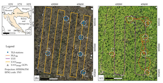
Figure 1.
The study area. (a) The location of the study area in Croatia; (b) leaf-off condition orthophoto from UAVimage dataset, unmanned aerial vehicle photogrammetry (UAVimage) trajectory and terrestrial laser scanning (TLS) stations; (c) unmanned aerial vehicle laser scanning (ULS) and handheld personal laser scanning (PLShh) trajectory on the leaf-on orthophoto produced from ULS onboard camera. Plot boundaries are represented by white circles in figure (b,c).
2.2. Remote Sensing Data Collection
Four different close-range remote sensing data sources were examined in this study; UAVimage, ULS, TLS and PLShh. The detailed information on the data collection is summarized in Table 1. The PLShh data collection included placing georeferencing spheres on previously surveyed and stabilized points, TLS included in situ planning of multi-scan positions and placing registration/georeferencing spheres, UAVimage included placing the ground control point (GCP) markers (it did not include a GCP survey) and ULS included inertial navigation system (INS) initialization.

Table 1.
Summary of used datasets.
2.2.1. Reference Data
A total station survey was conducted to obtain coordinates of topographic checkpoints that would be used as topographic reference for the DTM evaluation, and also to obtain coordinates of stabilized wooden stakes which were further used to georeference close-range remote sensing data (UAVimage, TLS and PLShh). Two total station surveys were conducted in total, first in February 2019 and, second, in January 2021. A Topcon es65 total station (Topcon Positioning Systems Inc., Tokyo, Japan), with 5” angle measurement accuracy, was used for both surveys. A permanent geodetic reference was established within the forest area during the first campaign, and polygons were stabilized in the cut tree stumps using metal bolts. A number of ground points on the plot were recorded within the same campaign; as well, wooden stakes (5 × 5 × 40 cm) were stabilized within the plot area. In total, 167 randomly chosen checkpoints and 18 stakes were recorded in six plots. The previously established geodetic reference was used in the second survey. The goal of the second survey was to determine coordinates of newly stabilized wooden stakes (5 × 5 × 40 cm) used as UAVimage control points and a TLS reference. The geodetic reference established in the first survey was used for the resection in the second survey, and the average resection positioning root mean square error (RMSE) value was 0.5 cm in the horizontal direction and 0.3 cm in the vertical direction. The small resection error indicated that the geodetic reference displacement between two epochs was small and could be neglected considering the values observed in this study.
2.2.2. UAVimage Data
The UAVimage acquisition was conducted on 19 March 2020, at the end of the leaf-off season, with the presence of some young leaves on hornbeams and also low vegetation. The UAV data were collected using a DJI Matrice 600 Pro (SZ DJI Technology Co. Ltd., Shenzhen, China) equipped with a stabilized Sony A7RII camera (Sony Corporation, Tokyo, Japan) and a Samyang 24 mm AF lens (Samyang Optics, Masan, South Korea). The timestamp of each exposure moment was recorded in a Receiver Independent Exchange Format (RINEX) file generated using an onboard Emlid Reach M+ GNSS receiver (Emlid, St. Petersburg, Russia), which was further used to calculate the exterior orientation (EO) position of images in the post-processing.
The flight was planned with 90% endlap and 80% sidelap, with a flying speed of 5 m∙s−1 at an altitude of 120 m, resulting in an approximately 2 cm ground sampling distance. During a single 10 min flight, a total of 269 images with 7952 × 5304 pixels resolution were taken. Five ground control points (GCPs) were stabilized using wooden stakes (5 × 5 × 40 cm) and signalized using A4 format paper checkerboard targets. The coordinates of the GCPs were determined in the second total station survey.
The EO positions of each exposure station were calculated in post-processing with RTKLib QT open-source software, relative to virtual reference station (VRS) data obtained via Geodetic Precise Positioning Service (GPPS) of Croatian Positioning System (CROPOS). Photogrammetric processing was carried out in Agisoft Metashape Version 1.6.5 (Agisoft LLC, St. Petersburg, Russia). Images were aligned using ground (GCPs) and aerial (EO positions) control and image tie points. The image tie points were generated at full resolution (parameter accuracy set to high), and the camera interior parameters were optimized within the bundle adjustment. Images were downsized by a factor of two (parameter quality set to high) and used to generate the dense point cloud, which resulted in point clouds with an average of ~2700 points∙m−2, and ~4 million points per plot.
2.2.3. Unmanned Aerial Vehicle Laser Scanning (ULS) Data
The ULS data were collected on 26 April 2019, during the early leaf-on period using a custom-made Y6 copter based on Arducopter open-source software. The UAV was equipped with a triple return LS Nano M8 LiDAR sensor (LIDAR SWISS, city, Switzerland), whose primary components are OxTS xNAV250 INS (Oxford Technical Solutions Ltd., Oxfordshire, UK), Quanergy M8 (Quanergy Systems Inc., Sunnyvale, CA, USA) and an onboard camera. Quanergy M8 operates at a 905 nm wavelength, has a 360° × 20° field of view with eight separate scan lines and a maximum range of 150 m with ±3 cm accuracy at 50 m distance. The angular resolution of 3 mrad results in a 10 cm radius footprint in the nadir direction and ellipses with 0.5 m lateral axes on the far end of the scan line.
Data were collected within a single 15 min flight at an altitude of 70 m and a flying speed of 5 m∙s−1. The LiDAR sensor unit was set to operate at 420 Hz pulse and 20 Hz frame rate, with ±50° off-nadir scan angles, and it resulted in an average of 285 points∙m−2. The resulting point cloud consisted of 84.14% of first, 15.59% of second and 0.27% of third returns. The angle step size of the LiDAR sensor was not specified by the manufacturer, therefore, after manual assessment, it was determined that the distances between the subsequent in-line points and scan lines at ground level were 18 and 6 cm and, based on the footprint size, provided full coverage at the ground level, given that there were no obstructions on the laser beam path. The ULS trajectory was obtained by post-processing INS/GNSS data using NAVsolve software (Oxford Technical Solutions Ltd., Oxfordshire, UK) and CROPOS VRS, followed by georeferencing point cloud using LS GEO-LAS software. Plot point clouds resulted in an average of 0.5 million points per plot (~400 points∙m−2).
2.2.4. Terrestrial Laser Scanning (TLS) Data
The TLS data were collected on 20 March 2020, a day after the UAVimage data collection; therefore, with the same phenological conditions. For the TLS data acquisition, a Faro FOCUS S70 (FARO Technologies Inc., Lake Marry, FL, USA) scanner with a multi-scan approach was used. The Faro FOCUS S70 scanner has 0.3 mrad beam divergence, ±1 mm ranging accuracy and a maximum ranging distance of 70 m. Six reference spheres with a 14.5 cm radius were set-up on wooden stakes whose coordinates were determined in the 2nd survey, and six scans per plot were collected (one central and five radial). The scan resolution was set to 1/4 and quality to 4×. Each scan lasted 5 min and the total time to scan the entire plot was approximately 30 min. The geometry of the multi-scan setup was primarily designed to record trees, not the terrain, which was intended to be a secondary product.
The collected scans were preprocessed in FARO SCENE (version 2020.0.5.5516) software. Reference spheres were marked manually and correspondences were found automatically, achieving a mean registration error of 1.1 mm. Scans were georeferenced in the software CloudCompare (version 2.11.3) using six parameter transformations (three rotations and three translations, average RMSE = 1.5 cm) based on the total station survey (second survey) of the sphere placement stakes. Five to six points were used for georeferencing each TLS point cloud, depending on the stake data availability. Each TLS point cloud consisted of more than 120 million points and was subsampled to 2 cm spacing to ease data manipulation and further processing, which resulted in fewer than 35 million points per plot (~28,000 points∙m−2).
2.2.5. Handheld Personal Laser Scanning (PLShh) Data
The PLShh data were collected using a GeoSLAM Horizon (GeoSlam Ltd, Nottinghamshire, UK) on 8 February 2019, during the leaf-off season, without any presence of low vegetation. GeoSLAM Horizon is an inertial measurement unit (IMU)-aided handheld laser scanning system based on the SLAM algorithm. The system consists of a rotating VLP-16 (Velodyne Lidar, San Jose, CA, USA) LiDAR sensor, IMU, data storage, and power supply. It does not have a GNSS sensor and all scans are recorded in the local coordinate system. The VLP-16 operates at a 903 nm wavelength, the angular step size is 0.1°–0.4° and it has 3 mrad beam divergence. Data collection across six plots was divided into three sessions. During the first session, only one plot was recorded (Plot 139), during the second session two plots were recorded (Plots 134 and 135) and during the third session, three plots (Plots 143, 141 and 140) were recorded (Figure 1). On average, data collection lasted 4 min per plot, including the time to walk in between the plots. The system operator was unfamiliar with the terrain and did not follow any predetermined path. The trajectory of the scanner can be seen in Figure 1.
The collected data were processed using the GeoSLAM HUB software, which generated the point cloud. The point cloud was georeferenced in a HTRS96/TM coordinate system using the software CloudCompare (version 2.11.3). Point clouds were georeferenced based on a six-parameter transformation (3 translations and 3 rotations) using spheres placed on the stakes whose coordinates were determined in the 1st survey. The point cloud from the first session was georeferenced using 3 spheres located on Plot 139 (RMSE = 0.7 cm); the point cloud from the second session was georeferenced using two spheres located on Plot 143 and another two spheres on Plot 140 (RMSE = 2.4 cm); the point cloud from the third session was georeferenced using two spheres on Plot 135 and two on Plot 134 (RMSE = 1.6 cm). The PLShh plot point cloud on average consisted of 36 million points (~ 28,500 points∙m−2).
2.3. Methods
Point clouds obtained using various close-range remote sensing methods were further processed to generate the regular 2D grid DTM. A morphological filtering algorithm and linear interpolation were used to produce the DTM, as presented in Liang et al. 2015 [28]. The lowest three-dimensional (3D) points in the regular grid were chosen as ground seed points. The seed points were grouped based on the connectivity of neighboring points. The largest group was classified as ground, and the ground was expanded based on the maximal expected slope and occlusion gap in the area. The DTM was generated based on classified ground points and linear interpolation. The same parameters were set for all datasets, i.e., the slope was gentle and maximal gap was set to 2 m. No manual editing was conducted on the point cloud, classification results or DTM. On average, 28.6%, 36.2%, 3.4% and 47.9% of the points were classified as a ground for TLS, PLShh, ULS and UAVimage data, respectively. A DTM grid at a resolution of 0.3 m was created from all datasets.
The DTMs estimated using different close-range remote sensing data sources were compared to checkpoints to evaluate the capacity of each system to produce high accuracy DTMs. Total station measurements are generally understood as the best ones available for DTM evaluation [10]. In total, 167 measurements were available within a 20 m distance from the plot center; there were 23, 27, 28, 27, 29 and 33 checkpoints at 6 plots, respectively.
Data normality and outliers were inspected, and accuracy measures for both normal and robust assessments were given, according to Höhle and Höhle [29]. The outliers were filtered out using three times the RMSE value, i.e., if the absolute value of discrepancy was greater than three times the RMSE, the measurement was removed from the dataset. Although non-robust statistics are frequently used to evaluate DTM [1,30], previous studies [26,29] have indicated that ALS and DAP errors rarely follow a normal distribution and can contain outliers; hence, the normality of the data was examined. Both graphical and numerical assessment were applied to test the data normality. For graphical assessment, Q-Q plots [19] (Appendix A, Figure A1), discrepancy histograms and theoretical normal distribution (Appendix A, Figure A2) were applied. Numerical data normality testing was based on the Shapiro–Wilk test p value. All tests indicated that neither dataset was normally distributed (p < 0.05) (Appendix A, Table A1). The non-robust and robust statistics were both calculated for the sake of comparison with other studies. The non-robust statistics were RMSE (Equation (1)), mean error (ME) (Equation (2)) and standard deviation (Equation (3)) as follows:
where is a discrepancy between the reference and estimated height, i is the checkpoint index, n is the total number of checkpoints and is an average discrepancy.
Robust statistics were median (Equation (4)), normalized median absolute deviation (NMAD) (Equation (5)), 68.3% quantile (Equation (6)) and 95% quantile (Equation (7)) as follows:
where Q denotes quantile and m denotes median.
The PLShh and TLS dataset results were analyzed to assess a relationship between achieved accuracy and the distance to the ground. The accuracy of the LiDAR devices depends on the distance to the object, and the object (reflecting properties, shape etc.) that laser beam reflects from. Therefore, it can be expected that distance to the ground might correlate with the achieved accuracy. The ranging accuracy decreases as distance to the ground increases, also, with increasing distance, the laser beam passes through more low vegetation before it hits the ground. The horizontal distance from each checkpoint to the nearest point of the PLShh trajectory and the TLS station was calculated using QGIS (version 3.16.2) software. In addition to the influence of the distance to the ground, i.e., checkpoint, we assessed the influence of interpolation in areas with no classified ground points on the accuracy of DTM reconstruction. Around each checkpoint, a 30 cm buffer had been created, and all checkpoints that did not have any classified ground point within 30 cm were labelled as interpolated based on nearby data. The analysis was conducted based on the statistics (Equations (1)–(7)) of all non-interpolated and interpolated points.
3. Results and Discussion
The height discrepancies of the close-range remote sensing data can be seen in Figure 2. It can be seen in Figure 2a,b that PLShh, TLS and UAVimage tend to overestimate ground, as well as that UAVimage and ULS have greater dispersion than PLShh and TLS. In addition, a few higher discrepancies indicate that outliers might be present in some datasets.
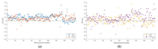
Figure 2.
Height discrepancies from reference data. (a) For PLShh and TLS; (b) For UAVimage and ULS.
After calculating non-robust and robust statistics, outliers were filtered out based on three times the RMSE value [29]. There were zero (0.00%%), one (0.00%), four (0.02%) and four (0.02%) detected outliers in PLShh, TLS, UAVimage and ULS data, respectively. After removing the detected outliers from the dataset, non-robust statistics were calculated once again.
In general, the accuracy measures are similar for all datasets (Table 2), especially for PLShh and TLS. Due to a small number of outliers, removal did not influence the statistics significantly. For outlier free datasets, the RMSE values range from 10 cm to 14 cm, and the ME values range from 0 cm to 8 cm. The PLShh and TLS have RMSE values of 10 and 11 cm, ME values of 7 and 8 cm and SD values of 6 and 7 cm, respectively; while the UAVimage and ULS have RMSE values of 14 and 9 cm, ME values of 8 and 0 cm and SD values of 12 and 9 cm, respectively. Concerning robust statistics, NMAD values of 5, 6, 9 and 10 cm, as well as median values of 7, 9, 7 and 0 cm were achieved for PLShh, TLS, UAVimage and ULS, respectively. The similar results obtained with PLShh and TLS are probably due to shared geometry, i.e., a terrestrial platform, whereas the slightly different results obtained with UAVimage and ULS, although both shared an airborne platform, are due to a different technology, i.e., photogrammetry and LiDAR.
Table 2.
Non-robust and robust statistics for close-range remote sensing datasets.
The difference in the performances of PLShh and TLS is negligible, which is unexpected considering that multi-scan TLS data is generally understood to be the best LiDAR data available and is typically used as reference data [25]. On the other hand, SLAM-based handheld laser scanners typically use low-cost sensors, resulting in data of a lower quality and increased noise. SLAM-based devices are also prone to drift due to a lack of features in sparse forests [21], but this did not occur in our case, which was confirmed by the high accuracy of the georeferencing data (RMSE ≤ 2.4 cm). The PLShh has an advantage in mobility, allowing it to record a larger area and reduce occlusions, which might have contributed to its accuracy. In contrast, TLS has high geometrical accuracy but visibility was hindered by low grass that was present during data acquisition, and it could be assumed that in the same conditions as in the PLShh dataset (February, no low vegetation), TLS would achieve slightly better results than those presented in this study.
The results of this study indicate that LiDAR technology, both terrestrial and UAV-based, performs better than UAV photogrammetry in forest areas. It is well known that LiDAR technology outperforms photogrammetry in dense forest areas, but it is still not clear how photogrammetry performs in leaf-off conditions. Only a few studies [24,25] have investigated the potential of UAV photogrammetry to provide a high accuracy DTM in leaf-off conditions. Photogrammetry is known to slightly overestimate terrain height in forest areas [1,19,24], and our results confirm such findings in deciduous forests. The presence of low grass in the study area during the time of acquisition certainly contributed to the overestimation, but similar results could be expected during most of the leaf-off period, namely, the ground is covered in a thick layer of dry leaves at the beginning of the leaf-off season, followed by snow. Snow compresses the leaves slightly and, after melting, the terrain surface is closest to the true ground and, soon, before the end of the leaf-off season, a low grass arises. Hence, the accuracy of the photogrammetric DTM in a broadleaved forest area can be improved only to a certain degree by aiming at a specific time period to collect the data, and further improvements have to be based on data collection and processing methodologies.
Moudrý et al. [24] assessed the accuracy of UAVimage- and ALS-derived DTM on 796 GNSS/RTK checkpoints in a steppe, aquatic vegetation area and forest area. In the forest area, RMSE values of 12 and 15 cm, NMAD values of 11 and 11 cm and ME values of 4 and 6 cm were reported for airborne LiDAR and UAVimage, respectively. Another study [1] assessed the accuracy of UAVimage and ULS derived DTM in a river levee. In total, 60 GNSS/RTK checkpoints were used to evaluate DTM in the area with the presence of low vegetation (below 20 cm), achieving ME values of 6 and 0 cm, and RMSE values of 14 and 11 cm, for UAVimage and ULS, respectively. The results of both studies are in agreement with our results, despite the use of different sensors and differences in the study areas. An international TLS benchmark study [27] investigated TLS based DTM estimation in different difficult conditions of the boreal forest. The DTM estimation method, which was also used in this study, achieved the best results (RMSE = 5 cm) for the plots with similar conditions.
Each evaluated data collection method has its advantages in forest area data collection; PLShh has great potential to deliver highly accurate DTM primarily due to its mobility, TLS provides highly accurate data with a narrow beam capable of penetrating dense vegetation during leaf-off conditions, UAVimage has a clear view of the ground from above and ULS has the capability of capturing both the crowns of the trees and ground below the trees.
One of the influences that might cause errors in PLShh and TLS data is the distance from an object, which translates to the return angle of the laser beam reflecting from the object, i.e., the more distant the object, the narrower the return angle. All checkpoints in our dataset were located within 20 m from the nearest TLS station and within 14 m from the nearest PLShh trajectory. Figure 3 displays the distance of checkpoints from the TLS station or PLShh trajectory with respect to deviations from the reference data. PLShh achieved consistent discrepancies through the whole dataset, with a slightly positive trend and with the majority lying in the range from 0 to 20 cm, with a few exceptions. A dense group of points in Figure 3a indicates that the mobility of PLShh is highly beneficial when DTM is produced from the data. Manual inspection of a few unexpected high discrepancies in the vicinity of the PLShh trajectory revealed that they were related to SLAM misregistration. TLS also displays a slightly positive trend and consistent dispersion. The trend is identical in both PLShh and TLS datasets and has a relatively low influence on terrain overestimation, i.e., overestimation starts at ~5 cm, and increases to 11 cm at a distance of 10 m, reaching 19 cm at a distance of 20 m. Manual examination of large discrepancies in the TLS data showed that the majority of checkpoints with large dispersion were occluded to most TLS stations and had a sparse point cloud nearby. Scan misregistration detected in PLShh data, which caused sporadic large discrepancies of the points near the trajectory, was not present in the TLS dataset, since TLS scans were registered with high accuracy using spheres.
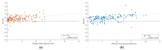
Figure 3.
Height discrepancies with respect to distance from (a) PLShh trajectory and (b) TLS stations.
These results indicate the equivalent performance of PLShh and TLS for DTM estimation. The lower geometrical accuracy of the PLShh is compensated for with mobility, thus the reduced ranging distance to the ground. In PLS, all the distances between trajectory and checkpoints were less than 14 m, where 90% of distances were less than 10 m and 50% were less than 3 m. In TLS, all distances were less than 20 m, where 90% of distances were less than 15 m and 50% of distances were less than 6 m. It is important to note that due to data acquisition in different time periods, TLS conditions were slightly more difficult than PLShh, thus TLS would probably achieve slightly better results if data were collected in the same period as PLShh.
Both TLS and PLS displayed good performances on the plot level. However, it can be assumed that PLShh would be more suitable for larger area scanning, especially when the trajectory is well planned in advance to sufficiently cover the area of interest.
TLS, PLShh and UAVimage are typically associated with high-density point clouds. It is important to note that a significant part of TLS, PLShh and ULS point clouds were not related to the ground, but vegetation as compared with UAVimage point clouds that lacked tree structure. All datasets, besides TLS, were collected from moving platforms, of which a typical benefit is the reduction of occlusions and gaps in the data, however, the significance of such a benefit is unclear. To make an assessment, we analyzed classified ground points of each dataset and observed how many checkpoints had classified ground points in the vicinity (<30 cm), i.e., if the DTM was interpolated at that specific point based on nearby data, or not. In total, 7, 3, 1 and 33 points with no classified ground points in the nearby area (<30 cm) were found in PLShh, TLS, UAVimage and ULS datasets, respectively. After excluding those points from the datasets, statistical results did show a slight improvement (Table 3) compared to statistics based on all points (Table 2), but the difference was negligible, which was expected for PLShh, TLS and UAVimage considering the small number of excluded points. However, ULS did not show a significant change after excluding ~20% of all checkpoints. These results indicate that linear interpolation is a safe technique for DTM interpolation in areas with no data, in a lowland deciduous forest, and it should also be noted that a high completeness of the data, for example, UAVimage, does not guarantee high accuracy.
Table 3.
Non-robust and robust statistics for close-range remote sensing datasets with excluded interpolated measurements.
The low number of excluded points for the PLShh and TLS dataset prove that despite the static platform, when planned correctly, multi-scan TLS data can provide high ground data completeness at the plot level.
4. Conclusions
This study assessed the capability of different close-range remote sensing techniques to estimate DTM in a lowland deciduous forest. In general, the studied close-range remote sensing data sources were capable of providing complete and reasonably accurate DTM in a lowland deciduous forest.
Four different data sources, PLShh, TLS, UAVimage and ULS, were investigated, and all of them achieved accuracy better than 15 cm for DTM estimation. All datasets, except ULS, systematically overestimated the terrain height at 7–9 cm level.
The TLS data are considered to be the highest quality LiDAR data, whereas compared to TLS, PLShh has low geometrical accuracy and high mobility. Yet, PLShh achieved results equivalent to TLS. Occlusions in TLS data can cause significant errors in DTM estimation, similar to SLAM misregistration effect in PLShh data. The distances from the scanner or trajectory were found to have a small influence on the DTM estimation accuracy.
The ULS and PLShh used the same grade of LiDAR sensor, but achieved different results. ULS had increased dispersion due to increased ranging distance and scanning geometry (direct view of the ground, minimal obstruction by the low grass), compared to PLShh.
UAVimage posed the lowest accuracy of all close-range remote sensing datasets, which is not surprising and can be primarily attributed to photogrammetry and the presence of low grass during the data acquisition. Nevertheless, UAVimage achieved relatively high accuracy and proved to be a suitable data source for DTM estimation in leaf-off forest conditions.
The completeness of the point cloud was found to be of low relevance on the lowland terrain. Studies with high-quality reference data have been rare until now but are important for establishing fundamental findings, thus, future studies should focus on evaluating close-range remote sensing technology for DTM estimation in different forest conditions, primarily the effects of the slope and vegetation type.
Author Contributions
Conceptualization, L.J., M.G., X.L. and I.B.; Funding acquisition, I.B.; Methodology, L.J.; Project administration, I.B.; Software, L.J. and X.L.; Supervision, X.L. and I.B.; Validation, L.J.; Writing—original draft, L.J.; Writing—review & editing, M.G., X.L. and I.B. All authors have read and agreed to the published version of the manuscript.
Funding
This research has been supported by projects “Retrieval of Information from Different Optical 3D Remote Sensing Sources for Use in Forest Inventory (3D-FORINVENT)” funded by the Croatian Science Foundation (HRZZ IP-2016-06-7686) and “Mogućnost primjene tehnologije ručnog laserskog skeniranja za procjenu drvne zalihe sastojina u glavnom prihodu” funded by the Scientific Research Program (ZIR) of Croatian Forests Ltd. The work of doctoral student Luka Jurjević has been supported in part by the “Young researchers’ career development project—training of doctoral students” of the Croatian Science Foundation funded by the European Union from the European Social Fund.
Institutional Review Board Statement
Not applicable.
Informed Consent Statement
Not applicable.
Acknowledgments
We would like to express our gratitude to the technicians of the Croatian Forest Research Institute who helped in setting-up and measurements of sampling plots, CADCOM d.o.o. for ULS data collection and GEOCENTAR d.o.o. for PLShh and TLS data collection.
Conflicts of Interest
The authors declare no conflict of interest.
Appendix A

Figure A1.
Q-Q plots for close-range remote sensing datasets. (a) PLShh; (b) TLS; (c) UAVimage; (d) ULS.
Figure A1.
Q-Q plots for close-range remote sensing datasets. (a) PLShh; (b) TLS; (c) UAVimage; (d) ULS.

Table A1.
Shapiro-Wilk normality test values.
Table A1.
Shapiro-Wilk normality test values.
| PLShh | TLS | UAVimage | ULS | |
|---|---|---|---|---|
| W | 0.95468 | 0.96050 | 0.91964 | 0.96847 |
| p | 0.00003 | 0.00011 | 0.00000 | 0.00075 |

Figure A2.
Histograms of height discrepancies from reference data for: (a) PLShh; (b) TLS; (c) UAVimage; (d) ULS. Red line represents the theoretical normal distribution.
Figure A2.
Histograms of height discrepancies from reference data for: (a) PLShh; (b) TLS; (c) UAVimage; (d) ULS. Red line represents the theoretical normal distribution.

References
- Salach, A.; Bakula, K.; Pilarska, M.; Ostrowski, W.; Górski, K.; Kurczynski, Z. Accuracy assessment of point clouds from LidaR and dense image matching acquired using the UAV platform for DTM creation. ISPRS Int. J. Geo Inf. 2018, 7, 342. [Google Scholar] [CrossRef]
- Niethammer, U.; James, M.R.; Rothmund, S.; Travelletti, J.; Joswig, M. UAV-based remote sensing of the Super-Sauze landslide: Evaluation and results. Eng. Geol. 2012. [Google Scholar] [CrossRef]
- Silva, B.M.; Silva, S.H.G.; de Oliveira, G.C.; Peters, P.H.C.R.; dos Santos, W.J.R.; Curi, N. Umidade do solo obtida por técnicas de mapeamento digital e sua validação de campo. Cienc. Agrotecnol. 2014, 38, 140–148. [Google Scholar] [CrossRef]
- Albrecht, C.M.; Fisher, C.; Freitag, M.; Hamann, H.F.; Pankanti, S.; Pezzutti, F.; Rossi, F. Learning and Recognizing Archeological Features from LiDAR Data. In Proceedings of the 2019 IEEE International Conference on Big Data (Big Data), Los Angeles, CA, USA, 9–12 December 2019; Institute of Electrical and Electronics Engineers Inc.: Piscataway, NJ, USA, 2019; pp. 5630–5636. [Google Scholar]
- Hyyppä, J.; Hyyppä, H.; Leckie, D.; Gougeon, F.; Yu, X.; Maltamo, M. Review of methods of small-footprint airborne laser scanning for extracting forest inventory data in boreal forests. Int. J. Remote Sens. 2008, 29, 1339–1366. [Google Scholar] [CrossRef]
- Balenović, I.; Jurjević, L.; Milas, A.S.; Gašparović, M. Testing the Applicability of the Official Croatian DTM for Normalization of UAV-based DSMs and Plot-level Tree Height Estimations in Lowland Forests. Croat. J. For. Eng. 2019, 40, 163–174. [Google Scholar]
- Maltamo, M.; Naesset, E.; Vauhkonen, J. Forestry applications of airborne laser scanning. Concepts Case Stud. Manag. For. Ecosyst. 2014, 27, 460. [Google Scholar]
- Jurjević, L.; Liang, X.; Gašparović, M.; Balenović, I. Is field-measured tree height as reliable as believed—Part II, A comparison study of tree height estimates from conventional field measurement and low-cost close-range remote sensing in a deciduous forest. ISPRS J. Photogramm. Remote Sens. 2020, 169, 227–241. [Google Scholar] [CrossRef]
- Pierzchała, M.; Talbot, B.; Astrup, R. Estimating soil displacement from timber extraction trails in steep terrain: Application of an unmanned aircraft for 3D modelling. Forests 2014, 5, 1212–1223. [Google Scholar] [CrossRef]
- Höhle, J.; Potuckova, M. Assessment of the quality of Digital Terrain Models. Off. Publ. EuroSDR 2011, 60, 85. [Google Scholar]
- Kaartinen, H.; Hyyppä, J.; Vastaranta, M.; Kukko, A.; Jaakkola, A.; Yu, X.; Pyörälä, J.; Liang, X.; Liu, J.; Wang, Y.; et al. Accuracy of Kinematic Positioning Using Global Satellite Navigation Systems under Forest Canopies. Forests 2015, 6, 3218–3236. [Google Scholar] [CrossRef]
- Baltsavias, E.P. A comparison between photogrammetry and laser scanning. ISPRS J. Photogramm. Remote Sens. 1999. [Google Scholar] [CrossRef]
- Baltsavias, E.; Gruen, A.; Eisenbeiss, H.; Zhang, L.; Waser, L.T. High-quality image matching and automated generation of 3D tree models. Int. J. Remote Sens. 2008. [Google Scholar] [CrossRef]
- Hyyppä, H.; Yu, X.; Hyyppä, J.; Kaartinen, H.; Kaasalainen, S.; Honkavaara, E.; Rönnholm, P. Factors affecting the quality of dtm generation in forested areas. Int. Arch. Photogramm. Remote Sens. Spat. Inf. Sci. 2005, 36, 85–90. [Google Scholar]
- Kraus, C.K.; Briese, M.; Attwenger, N.P. Quality measures for digital terrain models. Int. Arch. Photogramm. Remote Sens. Spat. Inf. Sci. 2004, XXXV-B2, 113–118. [Google Scholar]
- Stereńczak, K.; Kozak, J. Evaluation of digital terrain models generated in forest conditions from airborne laser scanning data acquired in two seasons. Scand. J. For. Res. 2011. [Google Scholar] [CrossRef]
- Debella-Gilo, M. Bare-earth extraction and DTM generation from photogrammetric point clouds including the use of an existing lower-resolution DTM. Int. J. Remote Sens. 2016, 37, 3104–3124. [Google Scholar] [CrossRef]
- White, J.C.; Coops, N.C.; Wulder, M.A.; Vastaranta, M.; Hilker, T.; Tompalski, P. Remote Sensing Technologies for Enhancing Forest Inventories: A Review. Can. J. Remote Sens. 2016, 42, 619–641. [Google Scholar] [CrossRef]
- Balenović, I.; Gašparović, M.; Milas, A.S.; Berta, A.; Seletković, A. Accuracy assessment of digital terrain models of lowland pedunculate oak forests derived from airborne laser scanning and photogrammetry. Croat. J. For. Eng. 2018, 39, 117–128. [Google Scholar]
- Liang, X.; Hyyppa, J.; Kukko, A.; Kaartinen, H.; Jaakkola, A.; Yu, X. The use of a mobile laser scanning system for mapping large forest plots. IEEE Geosci. Remote Sens. Lett. 2014, 11, 1504–1508. [Google Scholar] [CrossRef]
- Qian, C.; Liu, H.; Tang, J.; Chen, Y.; Kaartinen, H.; Kukko, A.; Zhu, L.; Liang, X.; Chen, L.; Hyyppä, J. An integrated GNSS/INS/LiDAR-SLAM positioning method for highly accurate forest stem mapping. Remote Sens. 2017, 9, 3. [Google Scholar] [CrossRef]
- Balenović, I.; Liang, X.; Jurjević, L.; Hyyppä, J.; Seletković, A.; Kukko, A. Hand-Held Personal Laser Scanning. Croat. J. For. Eng. 2021, 42. [Google Scholar] [CrossRef]
- Liang, X.; Kankare, V.; Hyyppä, J.; Wang, Y.; Kukko, A.; Haggrén, H.; Yu, X.; Kaartinen, H.; Jaakkola, A.; Guan, F.; et al. Terrestrial laser scanning in forest inventories. ISPRS J. Photogramm. Remote Sens. 2016. [Google Scholar] [CrossRef]
- Moudrý, V.; Gdulová, K.; Fogl, M.; Klápště, P.; Urban, R.; Komárek, J.; Moudrá, L.; Štroner, M.; Barták, V.; Solský, M. Comparison of leaf-off and leaf-on combined UAV imagery and airborne LiDAR for assessment of a post-mining site terrain and vegetation structure: Prospects for monitoring hazards and restoration success. Appl. Geogr. 2019, 104, 32–41. [Google Scholar] [CrossRef]
- Aguilar, F.J.; Rivas, J.R.; Nemmaoui, A.; Peñalver, A.; Aguilar, M.A. UAV-based digital terrain model generation under leaf-off conditions to support teak plantations inventories in tropical dry forests. A case of the coastal region of Ecuador. Sensors 2019, 19, 1934. [Google Scholar] [CrossRef]
- Debella-Gilo, M. Bare-earth extraction and dtm generation from photogrammetric point clouds with a partial use of an existing lower resolution DTM. In Proceedings of the International Archives of the Photogrammetry, Remote Sensing and Spatial Information Sciences—ISPRS Archives, Prague, Cezch Republic, 12–19 July 2016. [Google Scholar]
- Liang, X.; Hyyppä, J.; Kaartinen, H.; Lehtomäki, M.; Pyörälä, J.; Pfeifer, N.; Holopainen, M.; Brolly, G.; Francesco, P.; Hackenberg, J.; et al. International benchmarking of terrestrial laser scanning approaches for forest inventories. ISPRS J. Photogramm. Remote Sens. 2018, 144, 137–179. [Google Scholar] [CrossRef]
- Liang, X.; Kukko, A.; Hyyppä, J.; Lehtomäki, M.; Pyörälä, J.; Yu, X.; Kaartinen, H.; Jaakkola, A.; Wang, Y. In-situ measurements from mobile platforms: An emerging approach to address the old challenges associated with forest inventories. ISPRS J. Photogramm. Remote Sens. 2018, 143, 97–107. [Google Scholar] [CrossRef]
- Höhle, J.; Höhle, M. Accuracy assessment of digital elevation models by means of robust statistical methods. ISPRS J. Photogramm. Remote Sens. 2009, 64, 398–406. [Google Scholar] [CrossRef]
- Höhle, J.; Potuckova, M. The EuroSDR Test: Checking and Improving of Digital Terrain Models; Gopher: Utrecht, The Netherlands, 2006. [Google Scholar]


Publisher’s Note: MDPI stays neutral with regard to jurisdictional claims in published maps and institutional affiliations. |
© 2021 by the authors. Licensee MDPI, Basel, Switzerland. This article is an open access article distributed under the terms and conditions of the Creative Commons Attribution (CC BY) license (https://creativecommons.org/licenses/by/4.0/).