Abstract
Deep learning technology has achieved great success in the field of remote sensing processing. However, the lack of tools for making deep learning samples with remote sensing images is a problem, so researchers have to rely on a small amount of existing public data sets that may influence the learning effect. Therefore, we developed an add-in (LabelRS) based on ArcGIS to help researchers make their own deep learning samples in a simple way. In this work, we proposed a feature merging strategy that enables LabelRS to automatically adapt to both sparsely distributed and densely distributed scenarios. LabelRS solves the problem of size diversity of the targets in remote sensing images through sliding windows. We have designed and built in multiple band stretching, image resampling, and gray level transformation algorithms for LabelRS to deal with the high spectral remote sensing images. In addition, the attached geographic information helps to achieve seamless conversion between natural samples, and geographic samples. To evaluate the reliability of LabelRS, we used its three sub-tools to make semantic segmentation, object detection and image classification samples, respectively. The experimental results show that LabelRS can produce deep learning samples with remote sensing images automatically and efficiently.
1. Introduction
With the development of artificial intelligence, deep learning has achieved great success in image classification [1,2], object detection [3,4], and semantic segmentation [5,6] tasks in the field of computer vision. At the same time, more and more researchers use technologies similar to convolutional neural networks (CNNs) to process and analyze remote sensing images. Compared with traditional image processing methods, deep learning has achieved state-of-the-art success. For example, Rezaee et al. [7] used AlexNet [8] for complex wetland classification, and the results show that the CNN is better than the random forest. Chen et al. [9] built an end-to-end aircraft detection framework using VGG16 and transfer learning. Wei et al. [10] regarded road extraction from remote sensing images as a semantic segmentation task and used boosting segmentation based on D-LinkNet [11] to enhance the robustness of the model. In addition, deep learning is also used for remote sensing image fusion [12,13] and image registration [14,15].
Samples are the foundation of deep learning. The quality and quantity of samples directly affect the accuracy and generalization ability of the model. Due to the dependence of deep learning technology on massive samples, making samples is always an important task that consumes a lot of manpower and time and relies on expert knowledge. At present, more and more researchers and institutions begin to pay attention to how to design and implement high-efficiency annotation methods and tools for images [16,17], video [18,19], text [20,21], and speech [22,23]. In the field of computer vision, representative tools and platforms include Labelme [24], LabelImg [25], Computer Vision Annotation Tool (CVAT) [26], RectLabel [27] and Labelbox [28]. A brief comparison between these annotation tools is shown in Table 1. These tools are fully functional and support the use of boxes, lines, dots, polygons, and bitmap brushes to label images and videos. Advanced commercial annotation tools also integrate project management, task collaboration, and deep learning functions. However, none of them support labeling multispectral remote sensing images. The main reason is that the processing of remote sensing images is very complicated. As the data volume of a remote sensing image is huge generally compared to ordinary natural images, ordinary annotation tools cannot complete basic image loading and display functions, not to mention complex tasks such as pyramid building, spatial reference conversion, and vector annotation.

Table 1.
Comparison between different annotation tools.
Without an effective and universal annotation tool for remote sensing images, researchers can only rely on existing public data sets, such as the UC Merced Land Use Dataset [30], WHU-RS19 [31], RSSCN7 [32], AID [33], Vaihingen dataset [34] and the DeepGlobe Land Cover Classification Challenge dataset [35]. But these data sets have limited categories. For example, WHU-RS19 and RSSCN7 contain 19 categories and 7 categories, respectively. In addition, they have specific image sources and spatial-temporal resolutions, and the quality of annotations is also uneven. These reasons show it difficult for the existing remote sensing data sets to meet the actual needs in complex scenarios. Therefore, it is definitely necessary to develop a universal remote sensing image annotation tool.
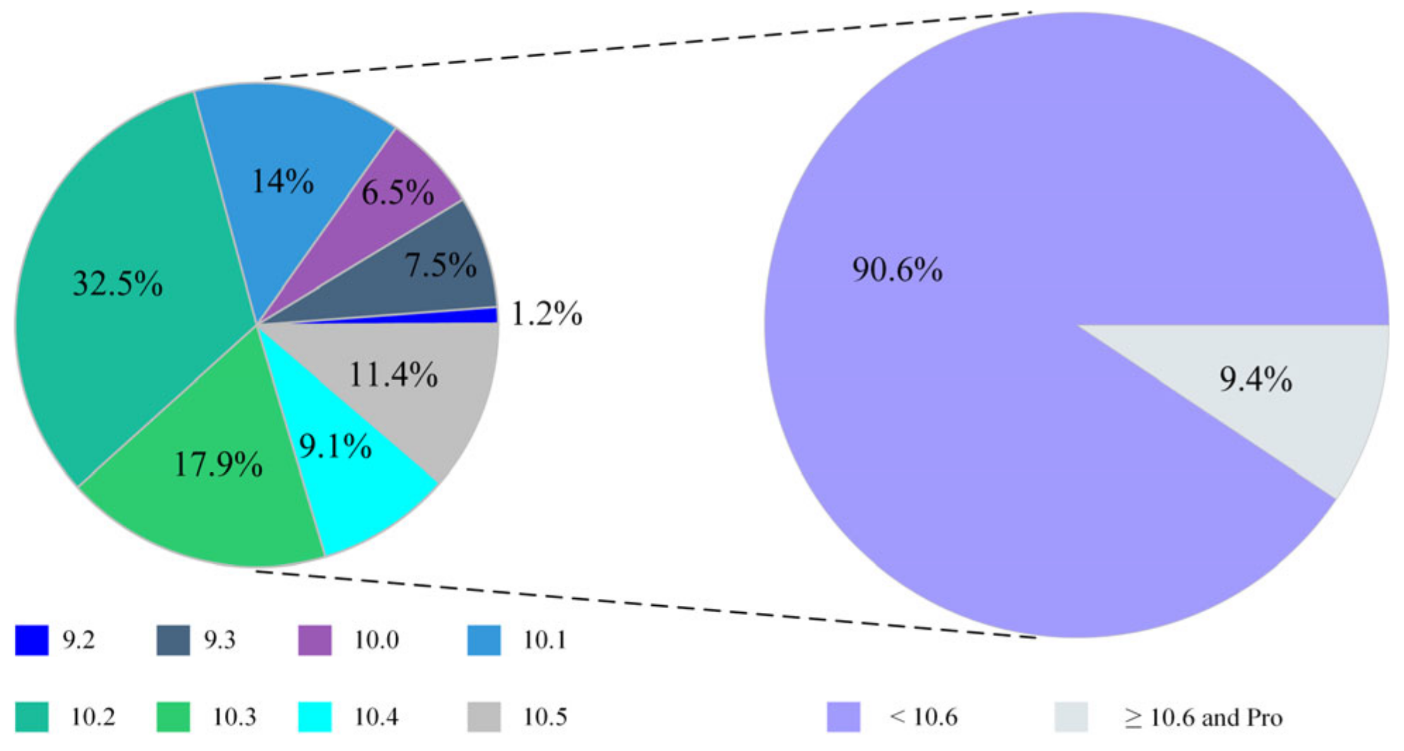
ArcGIS is one of the most representative software in geography, earth sciences, environment, and other related disciplines. It has diverse functions like huge image display, data processing, spatial analysis, and thematic mapping. Although the high version (ArcGIS 10.6) has added the function of making deep learning samples, there are still obvious limitations, such as (1) the tool cannot be used in lower versions of ArcGIS. We used “ArcGIS + version number” and “ArcMap + version number” as keywords and retrieved a total of 765 related papers in the past three years from the Web of Science (WoS). We counted the ArcGIS versions used in these papers, as shown in Figure 1. More than 90% of ArcGIS currently used does not have the function of making deep learning samples, and ArcGIS 10.2 and 10.3 are still the mainstream versions. (2) Output format restriction. The tool does not consider the high color depth and multiple bands of remote sensing images, which results in the format of the output sample must be consistent with the input. (3) The target size and distribution patterns are ignored. (4) Poor flexibility. The sample creation tool in ArcGIS requires that the input vector layers must follow a training sample format as generated by the ArcGIS image classification tool.

Figure 1.
Distribution of ArcGIS versions used by researchers.
According to the above analysis and considering both the development cost and the use cost, we developed the annotation tool LabelRS for remote sensing images based on ArcGIS 10.2. LabelRS enables researchers to easily and efficiently make remote sensing samples for computer vision tasks such as semantic segmentation, object detection, and image classification. Specifically, our tool supports inputting multispectral images with arbitrary bands and adapts to both sparse and densely distributed scenarios through a feature merging strategy. LabelRS solves the scaling problem of objects of different sizes through a sliding window. And a variety of band stretching, image resampling, and gray level transformation algorithms are used to enable the output samples to meet the actual needs of users and reduce the workload of postprocessing. In addition, we designed XML files to store metadata information to ensure the traceability of the samples. Each sample contains a spatial coordinate file to seamlessly realize the conversion between ordinary images and geographic images. More importantly, the sample production process we designed can also be potentially used to unravel many other problems of multispectral image classification, such as mineral recognition from X-ray maps [36,37] and breast cancer diagnosis from medical images [38]. All of them have a high spectral and spatial resolution, changing the reading and writing way of images according to the type of images can support the migration and reuse of LabelRS.
The main contributions of our work are summarized as follows.
- 1.
- An efficient framework is proposed to make deep learning samples using multispectral remote sensing images, which contains sub-tools as semantic segmentation, object detection, and image classification. To our knowledge, it is the first complete framework for image annotation with remote sensing images.
- 2.
- LabelRS is fully developed and implemented, and it is open-source and freely downloadable at https://github.com/junjieliwhu/LabelRS (accessed on 12 May 2021).
- 3.
- Three cases are implemented to evaluate the reliability of LabelRS, and the experimental results show that LabelRS can automatically and efficiently produce deep learning samples for remote sensing images.
2. Functionality and Implementation
The LabelRS toolbox we designed contains three sub-tools, namely Semantic Segmentation Tool, Object Detection Tool, and Image Classification Tool. Section 2.1 firstly introduces the design principles and functions of these three aspects, and then Section 2.2 introduces the specific implementation, including the interface design and input parameters of these tools.
2.1. Principle and Functionality
2.1.1. Semantic Segmentation
The left part of Figure 2 shows the processing flow of the semantic segmentation module. In addition to remote sensing images, the input of the tool also requires a vector file of the region of interests, and a field indicates the categories of different features. Such vector files can be drawn by users themselves in ArcGIS or other GIS tools, can be derived from NDVI [39] or NDWI [40], or can be derived from land survey data or other opensource geographic data, such as OpenStreetMap [41].
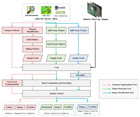
Figure 2.
Processing flow of LabelRS.
- (1)
- Feature Merging Strategy
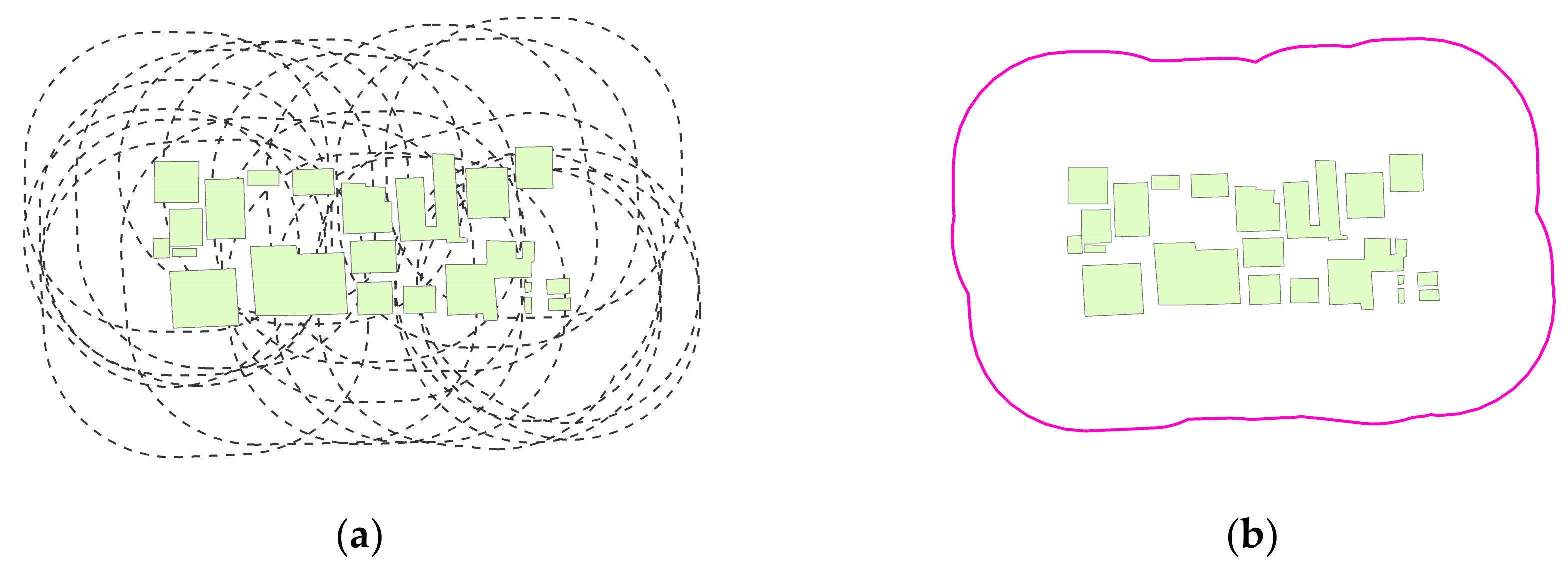
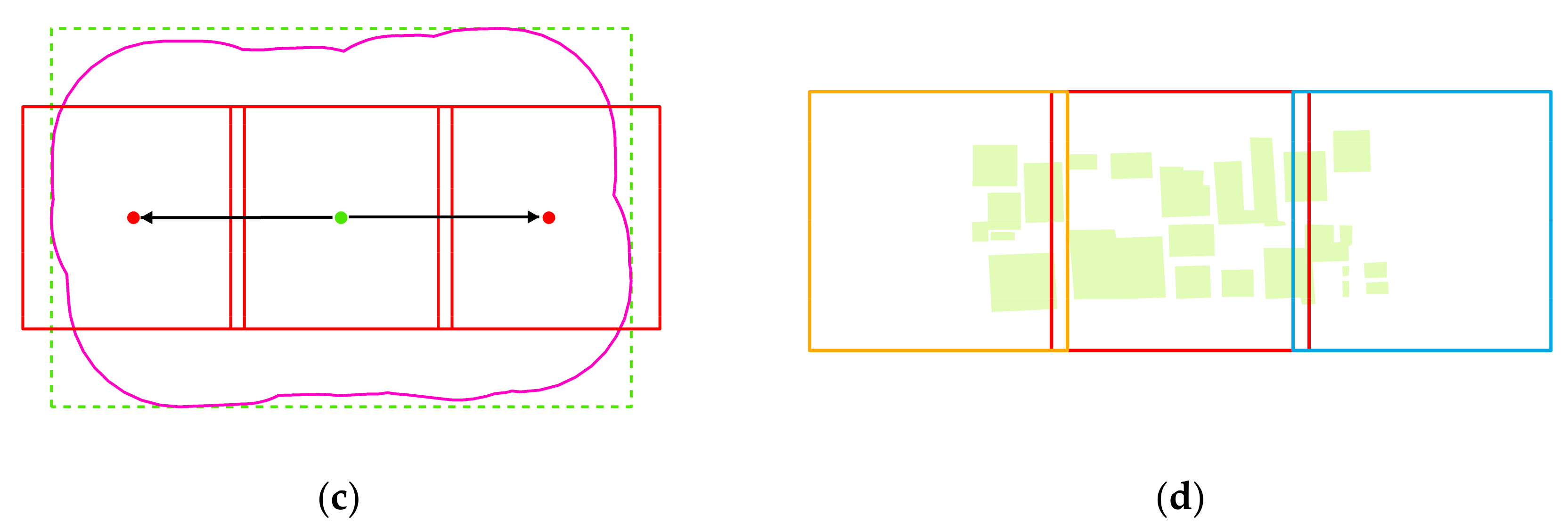
We divide the distribution patterns of objects into sparse distribution and dense distribution, as shown in Figure 3. Figure 3a shows dense buildings, and Figure 3b shows sparse ponds. For densely distributed objects, if each object is processed separately, a lot of computing resources will be consumed, and the generated samples have much redundancy and overlap. To solve this problem, we proposed a strategy of merging features, as shown in Figure 4. First, create a buffer on the outside of each object. The buffer of the building in Figure 3a is shown in Figure 4a. The radius of the buffer depends on the input sample size and the spatial resolution of the image. The calculation formula of the radius d is defined as:
where r is the spatial resolution of the image in the vertical or horizontal direction. It represents the spatial range represented by each pixel and can be obtained by reading the metadata of the image. t represents the sample size input by the user, and the unit of t is pixel. Then, the overlapping buffers are merged, and the obtained range is shown in Figure 4b. Finally, the densely distributed targets become independent objects.
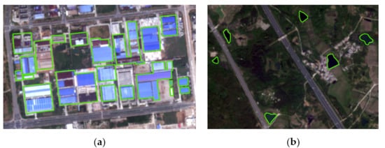
Figure 3.
Example of dense distribution and sparse distribution. (a) Dense distribution. (b) Sparse distribution.
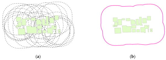
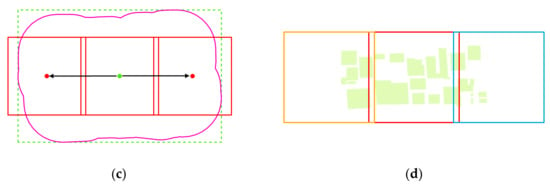
Figure 4.
Feature merging strategy. (a) Create buffers. (b) Merge buffers. (c) Sliding window. (d) Sample grids.
- (2)
- Split Large Targets
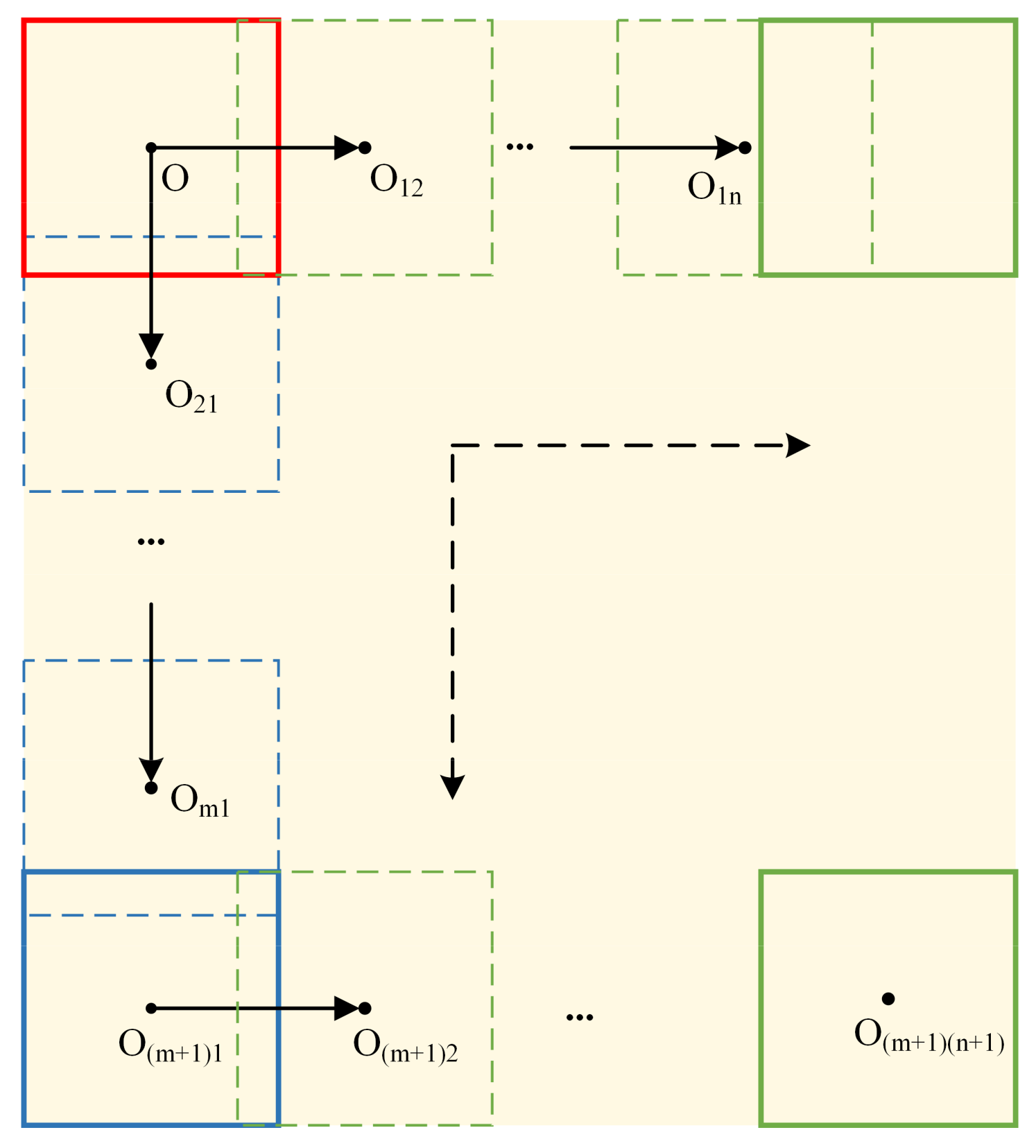
The independent objects are divided into three parts according to their size, as shown in Figure 5. We use the sliding window algorithm to split the target. First, determine the relationship between the height h, width w of the target envelop, and the sample size t. If h < 2t and w < 2t, take the center of the envelop as the sample center and r × t as the side length to construct a square as the range of the output sample. If h < 2t and w ≥ 2t, take the center of the envelop as the sample center O, and then slide left and right respectively. Set the center point after sliding as O’, then O’ can be calculated as follows:
where x and y represent the longitude and latitude of the sample center, respectively. m is the overlap size defined by the user. If h ≥ 2t and w < 2t, then slide up and down respectively, the principle is similar to the above. In the above two cases, we choose to start from the center of the envelop instead of starting from the upper left corner. This is really necessary because we found that when sliding from the upper left corner, the original complete object would be very fragmented. Starting from the center can guarantee its original distribution patterns to the greatest extent. Finally, if h > 2t and w > 2t, start from the upper left corner of the envelop and slide to the right and down, respectively, to generate the sample area. The detailed sliding window algorithm for semantic segmentation is also given in Algorithm 1. In addition, a potential problem with the above process is that when the boundaries of vector features are very complicated, creating buffers and fusing buffers will be very time-consuming. Therefore, another innovation of this paper is to use the Douglas-Peucker Algorithm [42] to simplify the polygons in the early stage. Our experiments show that for irregular objects with complex boundaries, the sample generation efficiency can be increased by more than 100 times after adding a simplified surface step.
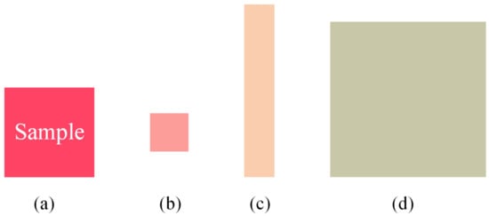
Figure 5.
Object categories. (a) Sample size. (b) Small objects. (c) Objects whose height or width is larger than the sample size. (d) Objects whose height and width are both larger than the sample size.
- (3)
- Band Combination and Stretching
The above steps create regular grids for making samples (we call them sample grids), and then these sample grids are used to crop the images and labels. Multispectral remote sensing images generally have more than three bands. Meanwhile, the pixel depth of remote sensing images is different from ordinary natural images and can usually reach 16BIT or 32BIT. But in the field of computer vision, natural images similar to JPEG and PNG are more common. Therefore, we allow users to choose the three bands mapped to RGB and set the image stretching method for multispectral images when users need to generate samples in JPEG or PNG formats. The image stretching algorithms we defined involves (1) Percentage Truncation Stretching (PTS). The algorithm needs to set the minimum percentage threshold minP and the maximum percentage threshold maxP. The two ends of the gray histogram of remote sensing images are usually noise. Assuming that the corresponding values of minP and maxP in the histogram are c and d, respectively. Then the stretched pixel can be calculated as follows:
where x is the pixel value before stretching. (2) Standard Deviation Stretching (SDS). It is similar to PTS, the difference is the calculation of c and d. The formula is as follows:
where m and s represent the mean and standard deviation of the band, respectively. k is a user-defined parameter, and the default value is 2.5. (3) Maximum and Minimum Stretching (MMS). The algorithm directly stretches the band linearly and maps the maximum and minimum values to 0 and 255, respectively.
- (4)
- Gray Level Transformation
Gray level transformation (GLT) is used to set the pixel value of the semantic segmentation label. We designed four GLT strategies to help users make the labels that they really need. (1) Default. The gray values of different types of features in the label are consistent with the attribute values of the input features. We default 0 as the background pixel. If the input shapefile uses 1 to represent the building, then the pixel value of the building area in the generated label is 1. This method requires that the field used to represent the category in the shapefile must be a short integer. (2) Maximum Contrast. Use gray values with maximum gaps to represent different categories. This method is suitable for visual display. For example, the input shapefile uses 1, 2, 3, and 4 to represent buildings, vegetation, water, and farmland, respectively. Then the pixel values of buildings, vegetation, water, and farmland areas in the output label are 63, 126, 189, and 252, respectively. (3) Positive Integer. It is suitable for non-numeric attribute values. For example, the input shapefile may use the string ‘water’ or the character ‘w’ to represent water bodies. In this case, the first two methods are invalid, and different types of features can be assigned from 1 in the order of positive integers. (4) Custom. Users customize the gray value of different types of features in the label. The above four different gray-level transformation methods will be recorded and saved in the output XML file.
- (5)
- Quality Control
The last step is quality control. Since we have created a buffer during the sliding and cropping process, part of the generated samples may not include any target or only a few pixels of the target, which will cause class imbalance and affect the training of the deep learning model. Therefore, we set a filter parameter f. If the ratio of foreground pixels to background pixels in the label is less than f, then the sample will be considered unqualified and discarded. Another problem is that the ‘no data’ area of the remote sensing images may be cropped, which will also be automatically identified and then eliminated.
In addition, different from the semantic segmentation samples in computer vision, spatial reference information is also an important component of remote sensing image samples. Therefore, we create jgw and pgw files for JPEG and PNG images, respectively, which are used to store the geographic coordinates of the upper left corner of the sample and the spatial resolution in the east-west and north-south directions. Finally, we use an XML file to record the metadata information of the sample to facilitate traceability and inspection.
| Algorithm 1. Sliding Window for Semantic Segmentation. |
| Input: polygon list PL, sample size t, image spatial resolution r, overlap size m output: sample grids SG 1 for each polygon Pi in PL 2 ex = Pi.GetExtent() 3 w, h, center = ex.width, ex.height,ex.center 4 if w < 2t and h <2t 5 grid = CreateSquare(center, t, r) 6 SG.append (grid) 7 elif w ≥ 2t and h < 2t 8 while center.x + t*r/2 > ex.Xmin 9 grid = CreateSquare(center, t, r) 10 SG.append (grid) 11 center.x = center.x − (t-m)*r 12 while center.x − t*r/2 < ex.Xmax 13 … 14 elif w < 2t and h ≥ 2t 15 … 16 else 17 center.x= ex.Xmin + t*r/2 18 center.y= ex.Ymax − t*r/2 19 while center.y + t*r/2 > ex.Ymin 20 while center.x − t*r/2 < ex.Xmax 21 grid = CreateSquare(center, t, r) 22 SG.append (grid) 23 center.x = center.x + (t-m)*r 24 center.y = center.y − (t-m)*r 25 center.x = ex.Xmin + t*r/2 26 return SG |
2.1.2. Object Detection
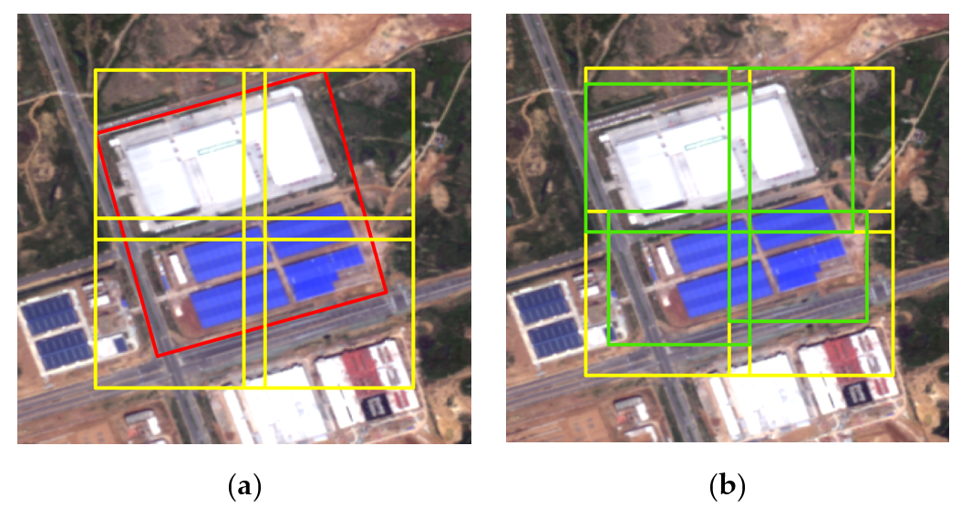
We first explain the related definitions. The entire image is regarded as a sample, and the coordinate range of the image is the sample range, as shown in the yellow box in Figure 6. The objects marked by the user in the sample are called targets or objects, as shown in the red box in Figure 6. The object detection tool is to separately record the sample range and target range of each labeled object. The processing flow of the object detection tool is shown in the middle of Figure 2. For the object detection samples, we are more concerned about the relationship between the sample size and the target size, and the position of the target in the sample. truncated is an important attribute of the sample in the object detection task. It represents the completeness of the target in the sample. If the target is completely within the image range, truncated = 0, indicating that no truncation has occurred. Suppose we want to generate samples with a size of 512 × 512, but the length and width of the target are greater than 512, then the target needs to be truncated, and each sample contains only a part of the target. Therefore, we first need to use the sliding window algorithm to segment large targets. Different from semantic segmentation, no buffer is created in the target detection tool, so the length and width of the object are compared with the size of the sample, rather than twice the size of the sample. Assuming that the red rectangle in Figure 7a is the target O marked by the user, and the grid obtained after segmentation using the sliding window is shown as the yellow rectangle in the figure, marked as G, then the calculation formula for truncated is as follow:
where Ti represents the truncation of the ith grid, S() is the function of calculating the area, and Gi is the ith grid. The actual labels of the targets after splitting are shown as the green rectangles in Figure 7b.
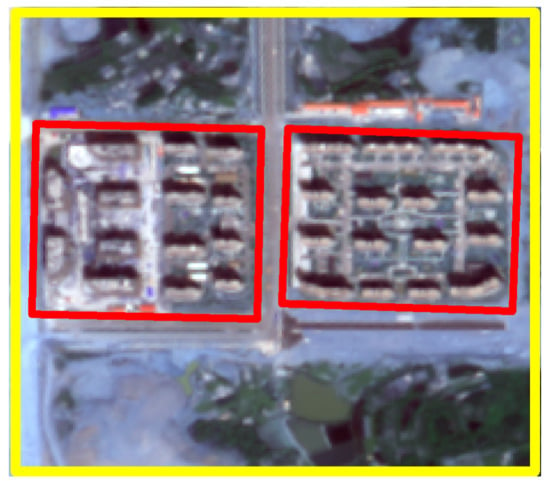
Figure 6.
The sample and object.
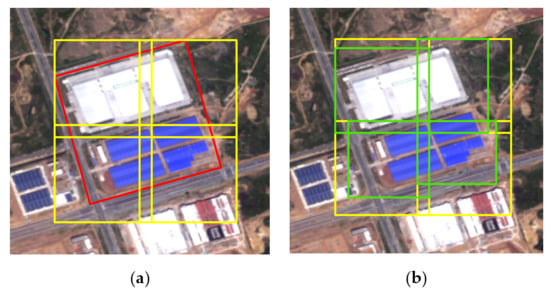
Figure 7.
Split the large target. (a) Split. (b) Labels of the targets after splitting.
Different from the pixel-level labeling of semantic segmentation, the object detection task needs to minimize the truncation of the target and ensure that the target is located in the center of the sample as much as possible. Therefore, a sample is made with each object as the center after segmenting the large target, and the sample may also contain other surrounding targets. In order to improve retrieval efficiency, we use t × r/2 as the radius for retrieval and only consider other targets within this radius. The calculated sample range is then used to crop the input image while recording the pixel position of the target in the sample. We have set up three currently popular metadata formats of object detection for users to choose from, namely PASCAL VOC [43], YOLO [4], and KITTI [44]. PASCAL VOC uses the xml file to store xmin, xmax, ymin, ymax, the category, and truncation value of each object. YOLO uses the txt file to store the category of each target, the normalized coordinates of the target center, and the normalized width and height of the target. KITTI is mainly used for autonomous driving and uses the txt file to store the category, truncation, and bounding box of each target. In addition, because the annotations are recorded in text, users cannot directly judge the quality of the annotations of the samples. We have designed a visualization function to superimpose the bounding box of the target onto the sample while creating samples and annotations so users can visually browse the annotation results.
2.1.3. Image Classification
In the image classification task, the entire image has only one value as a label, and there is no specific object position information. Therefore, the biggest difference between the above two tools is that other pixel information cannot be introduced during the splitting process. The processing flow of the image classification tool is shown in the right of Figure 2. First, segment the large target, as shown in Figure 8. Swipe to the right and down from the upper left corner of the target, then fill in from the right to left or bottom to top when the distance to the right or the bottom is less than the size of a sample. This can guarantee the integrity of the target without introducing new image information. Objects smaller than the sample will be resampled to the sample size. We set up three interpolation methods, Nearest, Bilinear, and Cubic, among which Nearest is simple and fast, but the result is rougher. Cubic generates smoother images, but the computational cost is high. Finally, the samples support arbitrary band combinations and stretching methods, and different types of samples are stored in different folders.
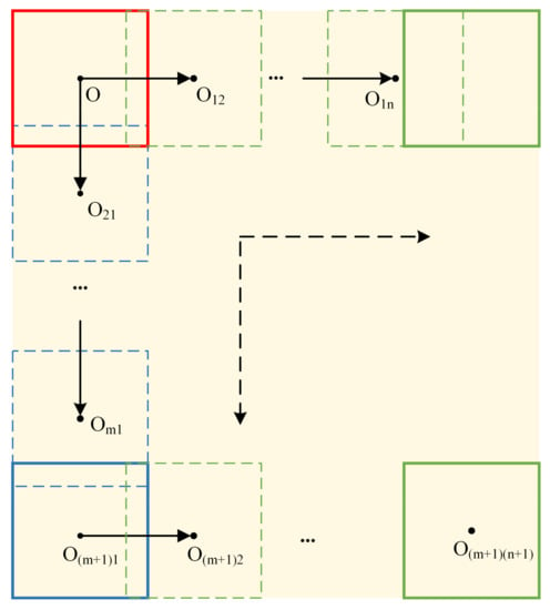
Figure 8.
Split the large target in image classification tool.
2.2. Implementation
Based on ArcGIS 10.2, we developed an upward compatible annotation tool LabelRS, for remote sensing images using Python 2.7. The python libraries imported by LabelRS mainly include ArcPy, OpenCV, and Pillow. LabelRS has two versions. One is the ArcGIS toolbox. Its advantage is that it has a visual graphical interface, which is convenient for parameter input and can be quickly integrated into ArcGIS. The other is Python scripts, which facilitate code debugging and integration. This version has higher flexibility and is more suitable for batch data processing environments. The following describes the implementation of the three sub-modules of LabelRS.
2.2.1. Semantic Segmentation Tool
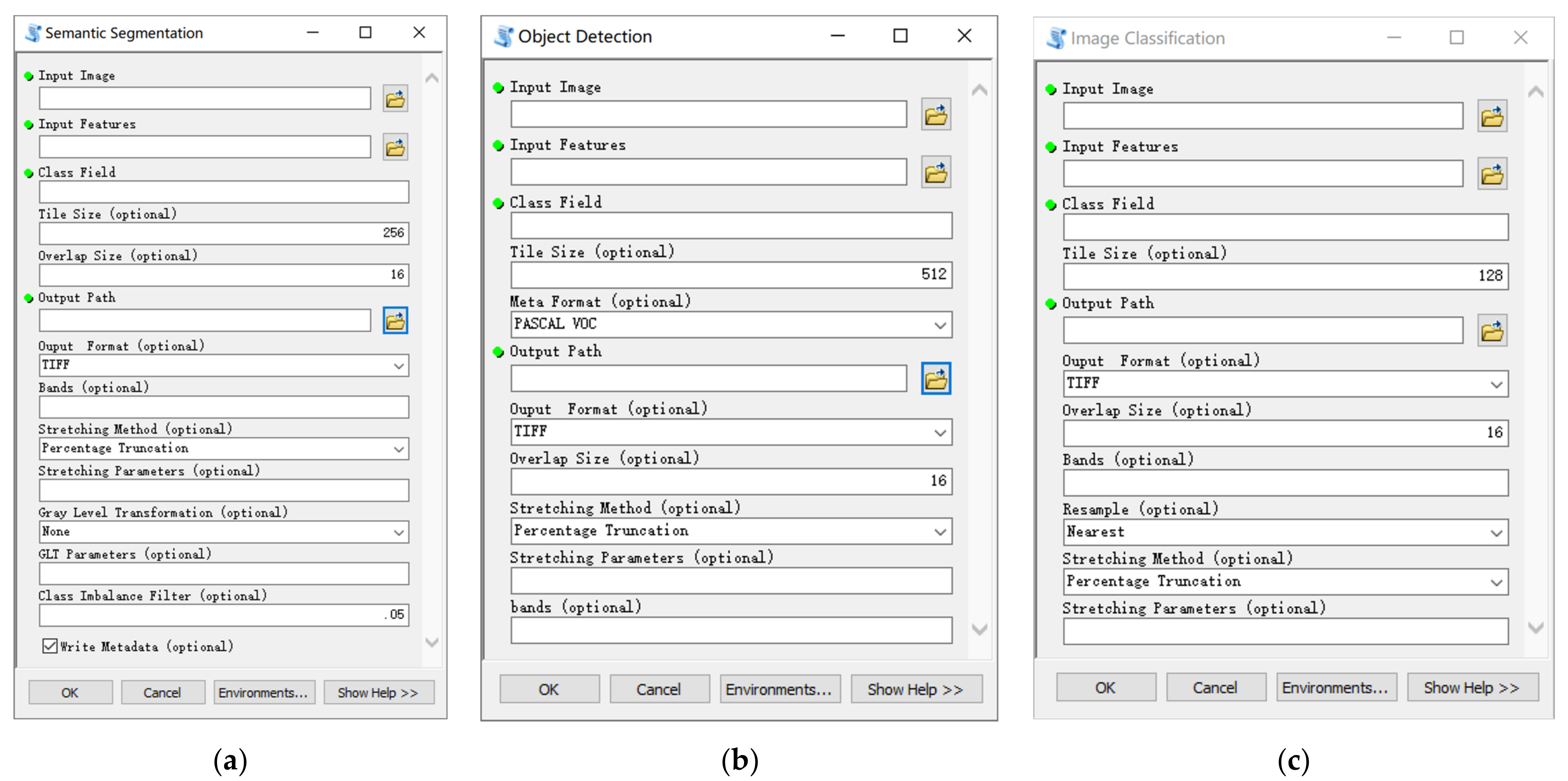
Dialog box of semantic segmentation tool is shown in Figure 9a. There are 14 input parameters in total, four of which are required. The meaning of each parameter is shown in Table 2.
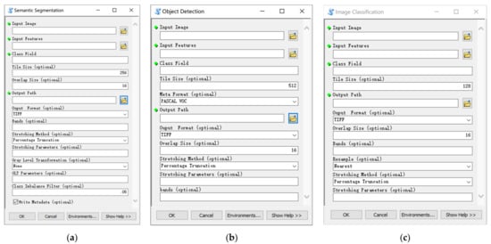
Figure 9.
Dialog boxes of LabelRS. (a) Semantic segmentation tool. (b) Object detection tool. (c) Image classification tool.

Table 2.
Input parameters of semantic segmentation tool.
2.2.2. Object Detection Tool
Dialog box of object detection tool is shown in Figure 9b. There are 11 input parameters in total, four of which are required. The meaning of each parameter is shown in Table 3.

Table 3.
Input parameters of object detection tool.
2.2.3. Image Classification Tool
Dialog box of image classification tool is shown in Figure 9c. There are 11 input parameters in total, 4 of which are required. The meaning of each parameter is shown in Table 4.

Table 4.
Input parameters of image classification tool.
3. Study Cases
3.1. Making Water Samples
Water is the most common and precious natural object on the surface [45]. Many researchers try to use deep learning methods to extract water bodies [46,47,48]. The boundary of the water body is very complicated, and manual labeling is time-consuming and labor-intensive. Therefore, we combined NDWI and LabelRS to propose an automated production process for water body samples. First, use the red and near-infrared band to calculate the NDWI, and then use the OTSU algorithm [49] to determine the segmentation threshold of water and non-water bodies. Filter out the interference of non-water objects such as farmland and mountain shadows through the area threshold. The finally obtained vector of water bodies can be input into the semantic segmentation tool to make water body samples.
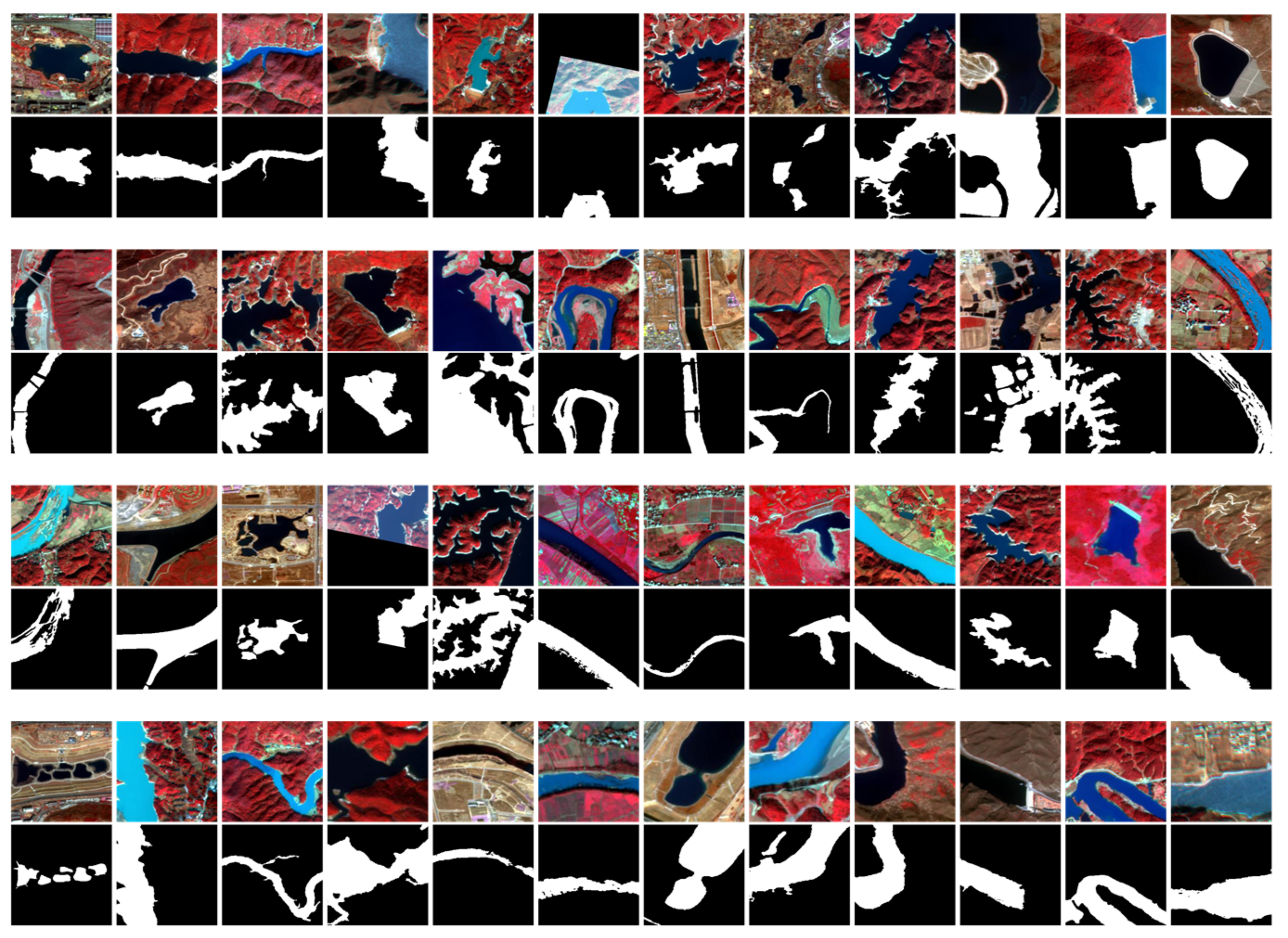
We used the GaoFen-2 (GF-2) satellite images, which have a spatial resolution of 4 m and contain four bands as red, green, blue, and near-infrared. The Beijing-Tianjin-Hebei region and Zhenjiang, Jiangsu Province were selected as the experimental areas. The climate types and land covers of these two regions are completely different. Due to the unique sensitivity of water to the near-infrared band, we chose the near-infrared, red, and green bands of GF-2 as the output wavebands of the sample. The sample size was set to 256. The gray level transformation method was Maximum Contrast, and the band stretching method was PTS. The experiment was carried out on a desktop computer, and the CPU was Intel Core i7-6700 3.40 GHz with 32 GB RAM. Finally, some samples made using semantic segmentation tools are shown in Figure 10. It can be seen that LabelRS combined with NDWI can segment the water body area well. The water body boundaries in the generated label are very detailed and smooth. Table 5 shows the processing time for a different task, and we can find that LabelRS is very efficient. The average time to produce a single multispectral remote sensing sample is 1–2 s.
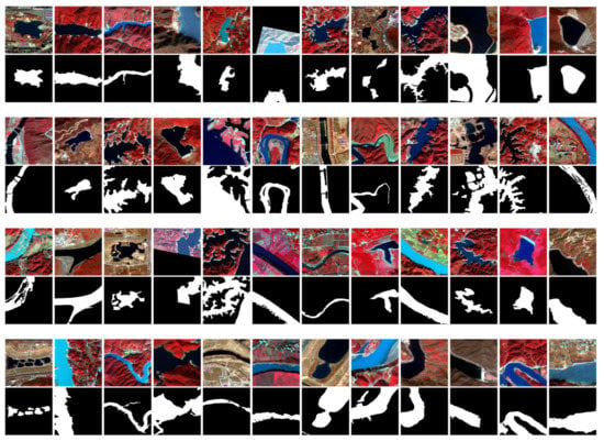
Figure 10.
Water samples.

Table 5.
Processing time of each sub-tool.
3.2. Making Dam Samples
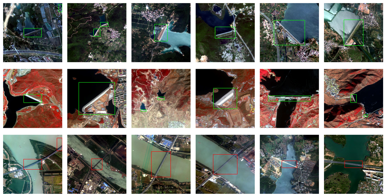
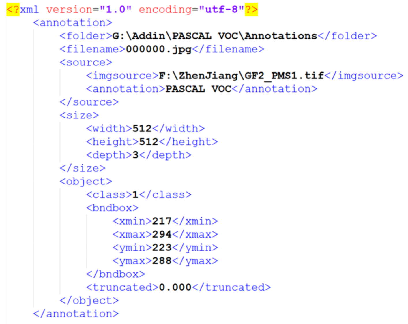
Dams are important water conservancy infrastructures with functions such as flood control, water supply, irrigation, hydroelectric power generation, and tourism. We chose the same experimental areas and data source as in the previous section. Due to the similarities between dams and bridges in geometric, spectral, and texture features, we treat bridges as negative samples. First, we manually marked the locations of dams and bridges in ArcGIS and saved them in a vector file. Then the object detection tool was used to make samples. The sample size was set to 512, and the metadata format was PASCAL VOC. In order to perform data augmentation, both true-color and false-color composite samples are generated, as shown in Figure 11. To visualize the labeling effect, the bounding boxes of dams and bridges have been drawn in different colors in the figure. Figure 12 is an example of PASCAL VOC annotation.
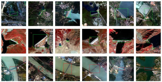
Figure 11.
Samples of dams and bridges, the green and red rectangle represent the bounding box of the dam and bridge respectively.
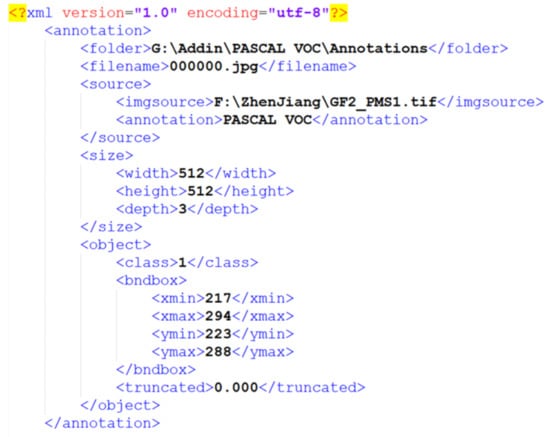
Figure 12.
Annotation of PASCAL VOC.
3.3. Making Land Cover Classification Samples
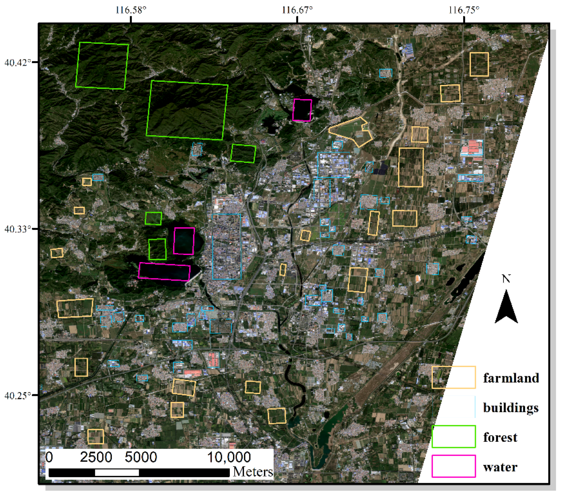
The classification of images at the image level instead of the pixel level means that we do not need to know the details of the distribution of the objects in the image. It is widely used in land use classification. We used Huairou District and Changping District in Beijing as experimental areas and selected GF-2 and GF-6 images as the main data sources. Figure 13 shows the main land use types in some parts of the experimental area. It can be seen that the main land cover classes include forest, water, buildings, and farmland. We first manually drew different features in ArcGIS software and then used the image classification tool of LabelRS to produce classification samples. The sample size was set to 128. The samples obtained are shown in Figure 14.
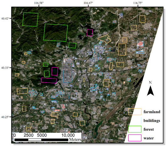
Figure 13.
Main land cover types in the test area.

Figure 14.
Land cover classification samples, from top to bottom are farmland, buildings, forest and water.
4. Conclusions
In response to the current lack of labeling tools for remote sensing images, we developed LabelRS based on ArcGIS and Python. Unlike normal images, remote sensing images have more bands, higher pixel depth, and larger breadth. The targets on remote sensing images also have different sizes and diverse distribution patterns. LabelRS has overcome these difficulties to a certain extent. It solves the problem of densely distributed targets by merging elements and divides large targets through sliding windows. A variety of band stretching, resampling, and gray level transformation algorithms are set to solve the problem of image spectral combination and pixel depth conversion. In addition, on the basis of conventional samples, unique spatial information is added to realize seamless conversion between natural samples and geographic samples. Our tool can assist researchers in making their own deep learning samples, which can reduce the burden of data preprocessing and the reliance on existing public samples, and ultimately helping researchers use deep learning techniques to solve specific target detection and recognition tasks. LabelRS also have certain limitations. (1) The object detection sub-tool does not support a rotating bounding box for the time being. (2) LabelRS currently rely on ArcPy scripts. Later we will use the GDAL library to achieve full open source. LabelRS’s current limitations are identified and will be the base for future developments.
Finally, we propose some suggestions on parameter settings. The first is how to choose adaptive tools. Large-size and irregular objects are not suitable for object detection because the rectangular bounding box may not effectively cover the target and will introduce a lot of interference. In this case, the semantic segmentation tool is more appropriate. The road map for selecting the tools is shown in Figure 15. The second is the sample size. The sample size for object detection can be set larger to avoid the target from being truncated. The sample size of image classification should be set as small as possible, because the larger the rectangle, the more non-label types of pixels may be introduced. The last is the output format. At present, most users are more accustomed to processing ordinary JPEG or PNG images. Because of this, LabelRS provides several useful data stretching functions to meet this demand. But in some cases, we prefer users to choose TIFF as the output format to avoid stretching the remote sensing images. For example, for a water body with uniform color, the image after stretching may look strange, which is caused by incorrect histogram truncation. In future research, we will continue to improve our code to make LabelRS easier to understand, easier to use, and easier to integrate.
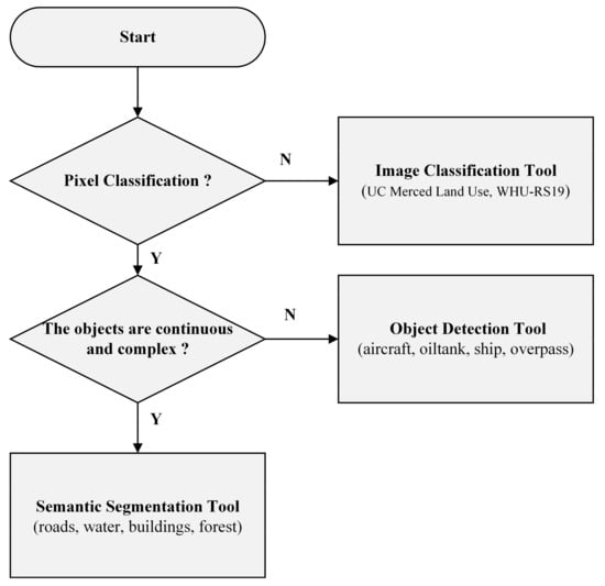
Figure 15.
The road map for selecting the tools.
Author Contributions
Conceptualization, J.L.; methodology, J.L. and C.T.; software, J.L.; validation, C.T., B.Y. and L.L.; formal analysis, J.L. and B.Y.; investigation, L.L.; resources, C.T.; data curation, J.L.; writing—original draft preparation, J.L.; writing—review and editing, L.M. and W.Z.; visualization, J.L.; supervision, L.M.; project administration, W.Z.; funding acquisition, L.M. All authors have read and agreed to the published version of the manuscript.
Funding
This research was funded by the Key Program of Open Foundation of Key Laboratory of National Geographic Census and Monitoring, Ministry of Natural Resources, grant number 2020NGCMZD01.
Data Availability Statement
LabelRS is open-source and freely downloadable at https://github.com/junjieliwhu/LabelRS (accessed on 12 May 2021).
Acknowledgments
The numerical calculations in this paper were performed on the supercomputing system at the Supercomputing Center of Wuhan University.
Conflicts of Interest
The authors declare no conflict of interest.
References
- Simonyan, K.; Zisserman, A. Very deep convolutional networks for large-scale image recognition. arXiv 2014, arXiv:1409.1556. [Google Scholar]
- He, K.; Zhang, X.; Ren, S.; Sun, J. Deep residual learning for image recognition. In Proceedings of the IEEE Conference on Computer Vision and Pattern Recognition, Las Vegas, NV, USA, 26 June–1 July 2016; pp. 770–778. [Google Scholar]
- Girshick, R.; Donahue, J.; Darrell, T.; Malik, J. Rich feature hierarchies for accurate object detection and semantic segmentation. In Proceedings of the 2014 IEEE Conference on Computer Vision and Pattern Recognition (CVPR), Columbus, OH, USA, 23–28 June 2014; pp. 580–587. [Google Scholar]
- Redmon, J.; Divvala, S.; Girshick, R.; Farhadi, A. You only look once: Unified, real-time object detection. In Proceedings of the IEEE Conference on Computer Vision and Pattern Recognition, Las Vegas, NV, USA, 26 June–1 July 2016; pp. 779–788. [Google Scholar]
- Long, J.; Shelhamer, E.; Darrell, T. Fully convolutional networks for semantic segmentation. In Proceedings of the 2015 IEEE Conference on Computer Vision and Pattern Recognition (CVPR), Boston, MA, USA, 7–12 June 2015; pp. 3431–3440. [Google Scholar]
- Ronneberger, O.; Fischer, P.; Brox, T. U-net: Convolutional networks for biomedical image segmentation. In International Conference on Medical Image Computing and Computer-Assisted Intervention; Springer: Cham, Switzerland, 2015; pp. 234–241. [Google Scholar]
- Rezaee, M.; Mahdianpari, M.; Zhang, Y.; Salehi, B. Deep convolutional neural network for complex wetland classification using optical remote sensing imagery. IEEE J. Sel. Top. Appl. Earth Obs. Remote Sens. 2018, 11, 3030–3039. [Google Scholar] [CrossRef]
- Krizhevsky, A.; Sutskever, I.; Hinton, G.E. Imagenet classification with deep convolutional neural networks. Adv. Neural Inf. Process. Syst. 2012, 25, 1097–1105. [Google Scholar] [CrossRef]
- Chen, Z.; Zhang, T.; Ouyang, C. End-to-end airplane detection using transfer learning in remote sensing images. Remote Sens. 2018, 10, 139. [Google Scholar] [CrossRef]
- Wei, Y.; Zhang, K.; Ji, S. Simultaneous road surface and centerline extraction from large-scale remote sensing images using CNN-based segmentation and tracing. IEEE Trans. Geosci. Remote Sens. 2020, 58, 8919–8931. [Google Scholar] [CrossRef]
- Zhou, L.; Zhang, C.; Wu, M. D-linknet: Linknet with pretrained encoder and dilated convolution for high resolution satellite imagery road extraction. In Proceedings of the 2018 IEEE CVF Conference on Computer Vision and Pattern Recognition Workshops (CVPRW), Salt Lake City, UT, USA, 18–22 June 2018; pp. 182–186. [Google Scholar]
- Masi, G.; Cozzolino, D.; Verdoliva, L.; Scarpa, G. Pansharpening by convolutional neural networks. Remote Sens. 2016, 8, 594. [Google Scholar] [CrossRef]
- Yuan, Q.; Wei, Y.; Meng, X.; Shen, H.; Zhang, L. A multiscale and multidepth convolutional neural network for remote sensing imagery pan-sharpening. IEEE J. Sel. Top. Appl. Earth Obs. Remote Sens. 2018, 11, 978–989. [Google Scholar] [CrossRef]
- Merkle, N.; Auer, S.; Müller, R.; Reinartz, P. Exploring the potential of conditional adversarial networks for optical and SAR image matching. IEEE J. Sel. Top. Appl. Earth Obs. Remote Sens. 2018, 11, 1811–1820. [Google Scholar] [CrossRef]
- Wang, S.; Quan, D.; Liang, X.; Ning, M.; Guo, Y.; Jiao, L. A deep learning framework for remote sensing image registration. ISPRS J. Photogram. Remote Sens. 2018, 145, 148–164. [Google Scholar] [CrossRef]
- Fiedler, N.; Bestmann, M.; Hendrich, N. Imagetagger: An open source online platform for collaborative image labeling. In Robot World Cup; Springer: Cham, Switzerland, 2018; pp. 162–169. [Google Scholar]
- Qin, X.; He, S.; Zhang, Z.; Dehghan, M.; Jagersand, M. Bylabel: A boundary based semi-automatic image annotation tool. In Proceedings of the 2018 IEEE Winter Conference on Applications of Computer Vision (WACV), Lake Tahoe, NV, USA, 12–15 March 2018; pp. 1804–1813. [Google Scholar]
- Dutta, A.; Zisserman, A. The VIA annotation software for images, audio and video. In Proceedings of the 27th ACM International Conference on Multimedia, New York, NY, USA, 15 October 2019; pp. 2276–2279. [Google Scholar]
- Shang, X.; Di, D.; Xiao, J.; Cao, Y.; Yang, X.; Chua, T.S. Annotating objects and relations in user-generated videos. In Proceedings of the 2019 on International Conference on Multimedia Retrieval, Ottawa, ON, Canada, 10–13 June 2019; pp. 279–287. [Google Scholar]
- Abrami, G.; Stoeckel, M.; Mehler, A. TextAnnotator: A UIMA based tool for the simultaneous and collaborative annotation of texts. In Proceedings of the 12th Language Resources and Evaluation Conference, Marseille, France, 13–15 May 2020; pp. 891–900. [Google Scholar]
- Wei, C.H.; Allot, A.; Leaman, R.; Lu, Z. PubTator central: Automated concept annotation for biomedical full text articles. Nucleic Acids Res. 2019, 47, W587–W593. [Google Scholar] [CrossRef] [PubMed]
- Grover, M.S.; Bamdev, P.; Kumar, Y.; Hama, M.; Shah, R.R. Audino: A Modern Annotation Tool for Audio and Speech. arXiv 2020, arXiv:2006.05236. [Google Scholar]
- Poletto, F.; Stranisci, M.; Sanguinetti, M.; Patti, V.; Bosco, C. Hate speech annotation: Analysis of an italian twitter corpus. In Proceedings of the 4th Italian Conference on Computational Linguistics, Rome, Italy, 11–12 December 2017; Volume 2006, pp. 1–6. [Google Scholar]
- Labelme: Image Polygonal Annotation with Python. Available online: https://github.com/wkentaro/labelme (accessed on 12 May 2021).
- LabelImg. Available online: https://github.com/tzutalin/labelImg (accessed on 12 May 2021).
- Computer Vision Annotation Tool (CVAT). Available online: https://github.com/openvinotoolkit/cvat (accessed on 12 May 2021).
- RectLabel. An Image Annotation Tool to Label Images for Bounding Box Object Detection and Segmentation. Available online: https://rectlabel.com (accessed on 12 May 2021).
- Labelbox: The Leading Training Data Platform for Data Labeling. Available online: https://labelbox.com (accessed on 12 May 2021).
- Image Annotation Tools: Which One to Pick in 2020. Available online: https://bohemian.ai/blog/image-annotation-tools-which-one-pick-2020 (accessed on 12 May 2021).
- Yang, Y.; Newsam, S. Bag-of-visual-words and spatial extensions for land-use classification. In Proceedings of the 18th SIGSPATIAL International Conference on Advances in Geographic Information Systems, San Jose, CA, USA, 2–5 November 2010; pp. 270–279. [Google Scholar]
- Xia, G.S.; Yang, W.; Delon, J.; Gousseau, Y.; Sun, H.; Maître, H. Structural high-resolution satellite image indexing. In Proceedings of the ISPRS TC VII Symposium-100 Years ISPRS, Vienna, Austria, 5–7 July 2010; Volume 38, pp. 298–303. [Google Scholar]
- Zou, Q.; Ni, L.; Zhang, T.; Wang, Q. Deep learning based feature selection for remote sensing scene classification. IEEE Geosci. Remote Sens. Lett. 2015, 12, 2321–2325. [Google Scholar] [CrossRef]
- Xia, G.-S.; Hu, J.; Hu, F.; Shi, B.; Bai, X.; Zhong, Y.; Zhang, L.; Lu, X. AID: A Benchmark Data Set for Performance Evaluation of Aerial Scene Classification. IEEE Trans. Geosci. Remote Sens. 2017, 55, 3965–3981. [Google Scholar] [CrossRef]
- Cramer, M. The DGPF-test on digital airborne camera evaluation overview and test design. Photogramm. Fernerkund. Geoinf. 2010, 75–84. [Google Scholar] [CrossRef] [PubMed]
- Demir, I.; Koperski, K.; Lindenbaum, D.; Pang, G.; Huang, J.; Basu, S.; Hughes, F.; Tuia, D.; Raskar, R. Deepglobe 2018: A challenge to parse the earth through satellite images. In Proceedings of the 2018 Conference on Computer Vision and Pattern Recognition, Salt Lake City, UT, USA, 18–22 June 2018; pp. 172–181. [Google Scholar]
- Launeau, P.; Cruden, A.R.; Bouchez, J.L. Mineral recognition in digital images of rocks: A new approach using multichannel classification. Can. Miner. 1994, 32, 919–933. [Google Scholar]
- Lanari, P.; Vho, A.; Bovay, T.; Airaghi, L.; Centrella, S. Quantitative Compositional Mapping of Mineral Phases by Electron Probe Micro-Analyser; Geological Society of London Special Publications: London, UK, 2019; Volume 478, pp. 39–63. [Google Scholar]
- Samala, R.K.; Chan, H.P.; Hadjiiski, L.; Helvie, M.A.; Richter, C.D.; Cha, K.H. Breast cancer diagnosis in digital breast tomosynthesis: Effects of training sample size on multi-stage transfer learning using deep neural nets. IEEE Trans. Med. Imaging 2018, 38, 686–696. [Google Scholar] [CrossRef]
- Carlson, T.N.; Ripley, D.A. On the relation between NDVI, fractional vegetation cover, and leaf area index. Remote Sens. Environ. 1997, 62, 241–252. [Google Scholar] [CrossRef]
- McFeeters, S.K. The use of the Normalized Difference Water Index (NDWI) in the delineation of open water features. Int. J. Remote Sens. 1996, 17, 1425–1432. [Google Scholar] [CrossRef]
- Haklay, M.; Weber, P. Openstreetmap: User-generated street maps. IEEE Pervasive Comput. 2008, 7, 12–18. [Google Scholar] [CrossRef]
- Visvalingam, M.; Whyatt, J.D. The Douglas-Peucker algorithm for line simplification: Re-evaluation through visualization. In Computer Graphics Forum; Blackwell Publishing Ltd.: Oxford, UK, 1990; Volume 9, pp. 213–225. [Google Scholar]
- Everingham, M.; van Gool, L.; Williams, C.K.; Winn, J.; Zisserman, A. The pascal visual object classes (voc) challenge. Int. J. Comput. Vis. 2010, 88, 303–338. [Google Scholar] [CrossRef]
- Geiger, A.; Lenz, P.; Stiller, C.; Urtasun, R. Vision meets robotics: The kitti dataset. Int. J. Robot. Res. 2013, 32, 1231–1237. [Google Scholar] [CrossRef]
- Prigent, C.; Papa, F.; Aires, F.; Jimenez, C.; Rossow, W.B.; Matthews, E. Changes in land surface water dynamics since the 1990s and relation to population pressure. Geophys. Res. Lett. 2010, 39. [Google Scholar] [CrossRef]
- Isikdogan, F.; Bovik, A.C.; Passalacqua, P. Surface water mapping by deep learning. IEEE J. Sel. Top. Appl. Earth Obs. Remote Sens. 2017, 10, 4909–4918. [Google Scholar] [CrossRef]
- Chen, Y.; Fan, R.; Yang, X.; Wang, J.; Latif, A. Extraction of urban water bodies from high-resolution remote-sensing imagery using deep learning. Water 2018, 10, 585. [Google Scholar] [CrossRef]
- Li, Z.; Wang, R.; Zhang, W.; Hu, F.; Meng, L. Multiscale Features Supported DeepLabV3+ Optimization Scheme for Accurate Water Semantic Segmentation. IEEE Access 2019, 7, 155787–155804. [Google Scholar] [CrossRef]
- Vala, H.J.; Baxi, A. A review on Otsu image segmentation algorithm. Int. J. Adv. Res. Comput. Eng. Technol. 2013, 2, 387–389. [Google Scholar]
Publisher’s Note: MDPI stays neutral with regard to jurisdictional claims in published maps and institutional affiliations. |
© 2021 by the authors. Licensee MDPI, Basel, Switzerland. This article is an open access article distributed under the terms and conditions of the Creative Commons Attribution (CC BY) license (https://creativecommons.org/licenses/by/4.0/).

