Abstract
Rivers play an essential role to humans and ecosystems, but they also burst their banks during floods, often causing extensive damage to crop, property, and loss of lives. This paper characterizes the 2014 flood of the Indus River in Pakistan using the US Army Corps of Engineers Hydrologic Engineering Centre River Analysis System (HEC-RAS) model, integrated into a geographic information system (GIS) and satellite images from Landsat-8. The model is used to estimate the spatial extent of the flood and assess the damage that it caused by examining changes to the different land-use/land-cover (LULC) types of the river basin. Extreme flows for different return periods were estimated using a flood frequency analysis using a log-Pearson III distribution, which the Kolmogorov–Smirnov (KS) test identified as the best distribution to characterize the flow regime of the Indus River at Taunsa Barrage. The output of the flood frequency analysis was then incorporated into the HEC-RAS model to determine the spatial extent of the 2014 flood, with the accuracy of this modelling approach assessed using images from the Moderate Resolution Imaging Spectroradiometer (MODIS). The results show that a supervised classification of the Landsat images was able to identify the LULC types of the study region with a high degree of accuracy, and that the most affected LULC was crop/agricultural land, of which 50% was affected by the 2014 flood. Finally, the hydraulic simulation of extent of the 2014 flood was found to visually compare very well with the MODIS image, and the surface area of floods of different return periods was calculated. This paper provides further evidence of the benefit of using a hydrological model and satellite images for flood mapping and for flood damage assessment to inform the development of risk mitigation strategies.
1. Introduction
Flooding is one of the most common environmental hazards, affecting many countries worldwide [1]. Pakistan, like many South Asian countries, is often severely impacted by flooding [2]. The Indus River is the longest river [2] and the most crucial water source in Pakistan, providing water to irrigate the land that produces 90% of the agricultural outputs of the country [3]. This river, however, often bursts its banks during the monsoon season, causing extensive damage to property and crops, as well as loss of lives. Droughts are also a recurrent feature in Pakistan, affecting agriculture, livelihoods, and the economy [4]. To better cope with the two extremes of the hydrological cycle, barrages and dams were built along the Indus River to store water during dry periods and to protect against the risk of flooding, respectively [5,6]. One such barrage is Taunsa Barrage, whose flood attenuation capability has decreased over the years due to severe sedimentation [7].
Flood mitigation is based on flood risk maps. The drawing of those maps is often based on the outputs of a hydrological model, which requires a digital elevation model (DEM) to represent the topographical surface and define a flood pathway [8]. A DEM can take the form of a digital terrain model (DTM) or a digital surface model (DSM). A DTM is a bare-Earth DEM [9]. Simultaneously, a DSM includes man-made features such as roads and buildings, vegetation, or any other features on the ground that can affect water flow [10]. The latter is particularly important in urban environments where a DSM is preferred for flood studies [11]. Data from various sources are used to develop a DEM, including land surveying, aerial photos, and, more commonly, remote sensing (RS) [9,10].
Flood risk mapping has seen the development of new applications over the years, notably the integration of hydrological models with RS in a geographic information system (GIS) [12]. The literature abounds in the use of GIS and RS in flood hazard mapping, for example [13,14,15,16], and more recently on using optical and radar satellite images to validate flood risk maps, for example [8]. Research in GIS and RS has since expanded from what was essentially the delineation of areas at risk of flooding to real-time monitoring of a flood and assessment of its impacts on population and infrastructure [17], and time and cost-effective crop loss assessment after a flood [18], notably for insurance purposes [19].
In 2014, heavy rains combined with glacier melting triggered flash flooding on the Indus River plains [7,20]. This was one of the worst river flooding disasters to affect the country, destroying crops, homes, and other infrastructure [21,22]. Given the Indus River basin exposure to flooding and the devastating impacts that this hazard causes, as well as the likelihood that flooding might increase in the future due to anthropogenic climate change [23], further research is needed to develop flood alleviation measures, including better flood monitoring. In this regard, satellite imagery has become increasingly important, particularly given improvements in image resolution, their processing in GIS, and the availability of 3D technology [24,25]. This paper presents an approach to map and assess the impacts of the 2014 flood of the Indus River in Pakistan using a hydrological model integrated within GIS and satellite images from Landsat-8. The simulated flood and its impacts are then compared with MODIS images, and recommendations are provided on mitigating future flood risks on the basics of the level of accuracy of the flooding simulations.
2. Materials and Methods
2.1. Study Area
The Indus River has its origins in the Tibetan Plateau; it flows through western China, the Ladakh region of India, and then enters Pakistan through the Gilgit-Baltistan region [4]. It continues its journey across the country’s entire length in a southerly direction to empty into the Arabian Sea near Sindh, the port of Karachi [26]. The river passes through the Muzaffargarh District of the Punjab region (Figure 1), which forms the focus of this study. This district comprises four subregions, with one of them bearing the same name as the district. To the north of the district is Taunsa Barrage, which was built to control the flow of the Indus River for irrigating agricultural land and for flood mitigation [27].
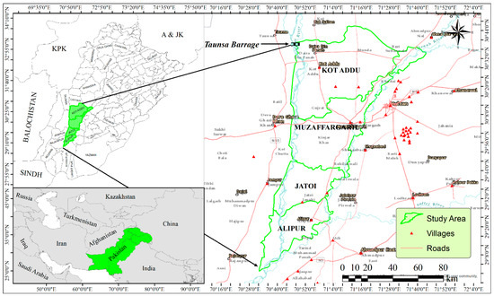
Figure 1.
The subdivisions of Muzaffargarh District in the Punjab province of Pakistan.
2.2. Data and Model
2.2.1. Remote Sensing Data for Land-Use/Land-Cover Type Classification
Images from the operational land imager (OLI) and thermal infrared sensor (TIRS) onboard the Landsat-8 satellite were obtained from the United States Geological Survey (USGS: http:/earthexplorer.usgs.gov/ (accessed on 6 March 2021)) to identify the land-use/land-cover (LULC) types of the river basin. The study area is covered by Path 151 of the Landsat-8 satellite, providing images at a temporal resolution of approximately 16 days. Three satellite images were obtained over the study area: before the flood (July 22), during the flood (August 7), and after it (September 24). Google Earth images were also obtained for comparison with the LULC types derived from the Landsat images.
2.2.2. The HEC-RAS Model and DEM Data
The US Army Corps of Engineers Hydrologic Engineering Centre River Analysis System (HEC-RAS) was applied to the study region to estimate the extent—and damage—of the 2014 flood. The n-values of Manning’s coefficient required by the model were based on the LULC type, with the LULC classification identified using the Landsat images mentioned above.
The HEC-GeoRAS GIS extension of the model comprises a set of procedures and tools for preparing geometric data for import into the HEC-RAS model to give a 3D view of the river basin, thereby allowing for an estimation of the spatial extent of a flood and its depth [28,29]. This import file requires a DTM represented by triangulated irregular networks (TIN). Each triangle represents a uniform slope steepness and flows direction. The DTM was created using data from the Shuttle Radar Topography Mission (SRTM) at 30 m resolution as distributed by the Consortium for Spatial Information (CSI). The study area in the dataset fell within one single tile. Several studies have used SRTM data to extract the boundary of a watershed and its drainage network [30,31]. This approach was followed, with the watershed delineated using the following steps in the GIS software ArcMap 10.6: i) importing the SRTM data, ii) creating a depression-less DTM over the study region, with the “Fill” method used to remove all sinks to create an accurate representation of flow direction, iii) determine the flow path for each cell in the DTM using a technique named “Flow Path,” and (iv) calculate the flow aggregation value at each cell given the number of upstream cells flowing into it. Depressions, also referred to as sinks, have no drainage due to being surrounded by cells at higher elevations and are often the result of DTM processing.
To represent the DTM as a TIN, points were extracted around the edge of the DTM spaces, and then, the surface was filled for each gap, creating a filled surface from the DTM. TINs were calculated from these points and converted to a base surface. The filled base surface from the TINs was subtracted from the filled surface from the DTM, and the result was added to the DTM base surface. The contour intervals were made over the area of interest, and the TIN was generated using these contours to create the geometric data.
2.2.3. Streamflow Data
Pakistan Water and Power Development Authority (WAPDA) provided discharge data for the Indus River at Taunsa Barrage from 1986 to 2014, which were used to identify the maximum daily discharge. The HEC-RAC model, however, requires as input the maximum instantaneous peak flow. As there is a lack of instantaneous peak flow data at the study location, it was estimated using Equation (1), a linear regression model based on 12 pairs of maximum instantaneous and maximum daily discharge data with a Pearson correlation coefficient of 0.94 [32]:
where Qp = maximum instantaneous discharge (m3-s−1) and QM = maximum daily discharge (m3-s−1). Table 1 depicts the resulting maximum instantaneous discharge at Taunsa Barrage.

Table 1.
Maximum instantaneous discharge (Qm) and maximum daily discharge (Qp) at Taunsa Barrage.
2.3. Methodology
2.3.1. LULC Classification
Figure 2 illustrates the methodological approach used in this study. The OLI Landsat-8 images were pre-processed using layer stacking and mosaicking. They were subject to atmospheric and radiometric correction with the sensor-specific information in the metadata file analyzed in ENVI v 5.4. In this process, spectral radiance was transformed to a planetary or exoatmospheric reflectance by normalizing solar irradiance to eliminate the influence of different solar zenith angles. The process accounted for different values of exoatmospheric solar irradiance resulting from the difference in a spectral band [33]. Atmospheric correction was also performed to remove the influence of ambient atmospheric conditions, including aerosols, thereby increasing the interpretability of the satellite image.
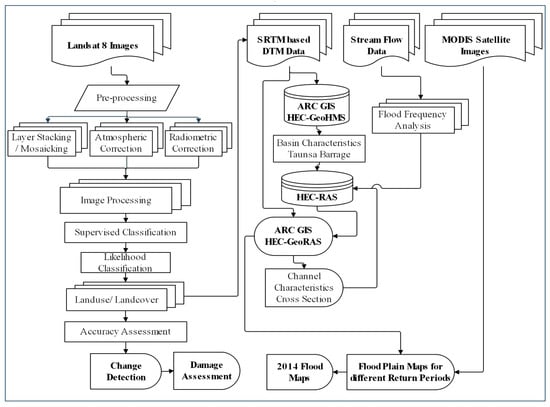
Figure 2.
Schematic representation of the methodological approach used in this study.
Radiometric correction is associated with a sensor that records the electromagnetic radiation intensity as a digital number (DN) for each pixel. These DNs may be translated to more practical real-life units such as radiance, reflectance, or temperature by using the sensor-specific information obtained from the metadata file of the Landsat image. Some software packages for image processing include radiometric calibration tools; for instance, Landsat-8 data can be translated to reflectance in ENVI v 5.4 without measuring the radiance first.
After atmospheric and radiometric corrections, ArcGIS 10.6 was used to perform a supervised classification on the Landsat images obtained before, during, and after the occurrence of the 2014 flood to identify the LULC types during each period (Figure 3) following the example of [34,35]. A maximum likelihood classification (MLC) [36,37] was also applied on the outcomes of the supervised classification, which resulted in a LULC classification with six categories, i.e., crop/agricultural land, built-up area, barren land, sand, water/wetland, and deposited material.
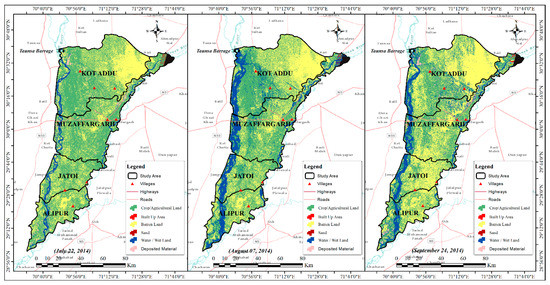
Figure 3.
LULC classification of Muzaffargarh District before the flood (left), during (middle), and after (right) the 2014 flood as identified using Landsat images.
2.3.2. Satellite-Based Flood Damage Assessment and Its Validation
Flood damage was assessed using a change detection technique, which consisted of calculating the surface area of the different LULC types of the watershed changing category because of the flood. For instance, an area shifting from “built-up area” or “agricultural/cropland” to “deposited material” in a satellite image obtained after the flood was considered a damaged area.
Google Earth images and a total of 212 samples with a minimum of 30 samples for each LULC type were collected by a team of WAPDA together with their GPS location. These were used to validate the LULC type classification after the flood. The verification was done at random points using the random sample points method in the ArcGIS Spatial Analyst extension. These points were then converted into KML format so that they could be displayed in Google Earth. The accuracy of the LULC type classification after the flood was then measured using 600 ArcGIS random points and the 212 GPS points.
Furthermore, 25 GPS points of the selected groups were used for the post-flood verification process. The accuracy of maps that depicted flooded areas was assessed using 440 ArcGIS random points on the Google Earth images and 160 GPS points, with the uncertainty matrix established using the results obtained from this comparison. The assessment was then quantified using the Kappa coefficient (K).
2.3.3. Mapping the Spatial Extent of Floods of Different Return Periods and Comparing the Extent of the 2014 Flood with MODIS Imagery
The floodplain maps were produced using the following steps: (1) a flood frequency analysis was performed to relate the discharge data at Taunsa Barrage to specific return periods; (2) development of the SRTM-based DTM model; (3) extract the boundary of the watershed and its drainage network; (4) prepare the geometric data using the HEC-GeoRAS extension; (5) run the HEC-RAS model to simulate river discharge; (6) produce floodplain maps for floods of various return periods using the peak discharge identified from the flood frequency analysis.
In the flood frequency analysis, the log-Pearson form III [38], the Gumbel [39,40], and the log-normal [41,42] distributions were fitted to the discharge data depicted in Table 1. The Kolmogorov–Smirnov (KS) test identified the log-Pearson III as the best distribution using the approach described in Khattak et al. [32]. The distribution was then used to estimate the peak discharge value for a flood of a given return period. This peak discharge value was input into the HEC-RAS model to map the extent of the flood.
The watershed characteristics, such as the river centerline, were extracted from the DTM using the Geospatial Hydrologic Modeling Extension of the HEC model (HEC-GeoHMS). Geometric data for the river, such as cross-sections and bank stations and flow direction lines, were prepared using HEC-GeoRAS. In addition to the DTM, geo-referenced natural-color images from Google Earth were obtained to estimate Manning’s roughness coefficient, a model parameter, for each of the relevant LULC categories (Table 2). For this, separate polygons were drawn for each LULC category and Manning’s roughness coefficient was calculated for each polygon using the method proposed by McCuen [43] and Chow et al. [20], while assigning a value of 0.32 for single-story and double-story houses [44]. After implementing all geometric data specifications and assigning Manning’s roughness coefficient values to each LULC category, the GIS file was imported into the HEC-RAS.
Table 2.
The estimated Manning’s n value for different land use categories.
The next step consisted of providing the steady flow and boundary conditions. For steady and unsteady analyses, standard depth is the most employed boundary state and, accordingly, the HEC-RAS model uses this value to estimate the depth of a flood. The energy slope can be estimated by calculating the slope of the river stretch downstream of the modeled river reach. To run an unsteady model, external boundary conditions are required. These are the boundary conditions that must be applied to the upstream and downstream ends of the river. Internal border requirements are optional and allow the user to identify gate operations and associated modifications to the flow along the length of the river.
The level of the flood along the different stretches of the river was simulated using the peak river flow introduced into the HEC-RAS model. This peak river discharge corresponded to floods with a return period of 5-, 10-, 50-, 100-, and 150-year, along with using the maximum instantaneous discharge value of the 2014 flood. The model produced as outputs the flow depth, the cross-sectional discharge, and other related data. After deleting all errors and after the water surface generation and floodplain delineation, the output file from HEC-RAS was imported into ArcGIS, and a floodplain map was produced. Only the flood depth could be obtained on this map; therefore, a smooth water surface was created.
The UNITAR Operational Satellite Application Network (UNOSAT) analyzed the 2014 Indus River flood using a MODIS image taken on July 31. This image was used to examine the extent of the flood and its damage and to compare it with that simulated by the model.
3. Results
3.1. Changes in LULC after the Flood and Assessment of Accuracy
Figure 3 illustrates the LULC types before the flood, during the flood, and after it. ‘Deposited material’ was not a LULC category for the image taken during the flood but only for the image after it. The change detection technique reveals significant changes for all LULC types. Before the flood, the watershed, covering a surface area of approximately 581.8 km2, consisted of 63.8% crop/agricultural land, 11.3% built-up area, 21.1% barren land, 0.9% sand, and 1.1% deposited material (Figure 4). The ‘Water/Wetlands’ category covered only 1.1% of the watershed area, but, as expected, this increased dramatically to 38% during the flood, therefore affecting other LULC types. Specifically, the ‘built-up’ LULC type decreased from 11.34 to 9.35%, the ‘crop/agricultural land’ category, which covers the largest surface area of the catchment, decreased from 63.8 to 55.9%, and the ‘barren land’ LULC type decreased from 21.1 to 17.2% because of the flood; hence explaining the extensive damage that the 2014 flood caused to crops and the built environment.
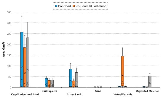
Figure 4.
Change in LULC in Muzaffargarh District according to Landsat 8 images before, during, and after the 2014 flood.
Different measures were used to assess the accuracy of the supervised and MLC classification to categorize the watershed into the six LULC types. The highest overall accuracy (OA) value, i.e., 96%, was obtained from the pre-flood image (July 22), while the post-flood image (September 24) had the lowest OA of 90%. The highest UA of the ‘built-up’ area class was attained for the pre-flood image, with a value of 98.98%, while the lowest was 80.11% for ‘water/wetland’ class for the image taken during the flood (August 8). The OA and K for Muzaffargarh District as a whole are 0.96 and 0.94 (corrected samples, 576), 0.93 and 0.91 (corrected samples, 545), 0.90 and 0.85 (corrected samples, 560) for the pre-flood, during the flood, and post-flood image, respectively (Table 3).
Table 3.
Accuracy assessment (%) of the LULC before, during, and after the 2014 flood.
Overall, the results reveal a high level of accuracy of the LULC categorization technique. For the pre-flood image, the highest UA, i.e., 98.98%, is attained for the ‘built-up area’ class, while the highest PA, also at 98.98%, is seen for the ‘crop/agricultural land’ LULC type. After the flood, the water category returned nearly to its original pre-flood level, decreasing from 38% to 1.87%. However, the percentage of the watershed covered by the ‘built-up’ LULC category did not return to its original value, but to only 9.35%. This is likely because after the flood water receded, materials were deposited, hence this category showed a significant increase from 1.10% to 15.04% in the post-flood image (Figure 4). An increase from 45.22% to 55.92% was also seen in the ‘crop/agricultural land’ category, while the ‘barren land’ LULC type, for its part, remained unchanged. The category defined as ‘sand’ increased marginally from 0.14 to 0.60%, as seen in Figure 3 (right image).
3.2. Damage Assessment
This study shows that the ‘crop/agricultural land’ was the most damaged LULC class because of the 2014 flood. Approximately 371.2 km2 of crop/agricultural land was inundated compared to 65.98 km2 for the built-up area. Furthermore, the results highlight that deposited material damaged about 45.91 km2 of agricultural/cropland and 11.57 km2 of built-up area (Figure 5).
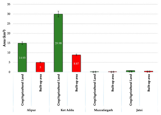
Figure 5.
Damage assessment to the ‘crop/agricultural land’ and ‘built-up areas’ LULC categories for each subdivision of the district following the 2014 flood.
3.3. Frequency Analysis
The maximal instantaneous discharges at Taunsa Barrage for floods of different return periods are indicated in Table 4 using the LN, Gumbel, and LP3 distributions, while Figure 6 depicts the discharge for each of those distributions. For the three distributions, the recorded discharge values are higher than those provided by [2]. The expected flood peaks using the LN distribution are larger than those obtained using the LP3 and Gumbel distributions for all return periods greater than 50 years. The K-S test results for Taunsa Barrage are shown in Table 5.
Table 4.
Maximum instantaneous discharge (m3s−1) according to the LN, Gumbel, and LP3 probability distributions at Taunsa Barrage for floods of various return periods.
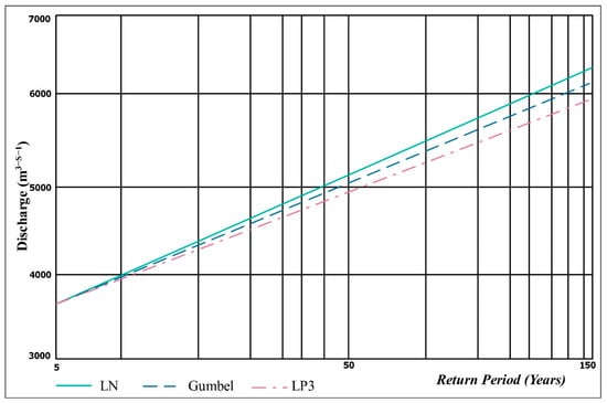
Figure 6.
The discharge of the Indus River at Taunsa Barrage using the log-Pearson type III, Gumbel, and log-normal probability distributions.
Table 5.
Result of the K-S statistical test at Taunsa Barrage.
The LP3 distribution was used to predict flood peaks at Taunsa Barrage based on the value of the K-S statistical test. For the return periods of 5-, 10-, 50-, 100-, and 150-year as well as for the 2014 flood, the instantaneous flows derived from the LP3 distribution were used as steady flow inputs into the HEC-RAS model. The first segment was downstream from lower Taunsa at some distance. The topography was comparatively precise compared to the upstream parts, while the second part was at the intersection of the Indus River. Both floods with 100- and 150-year return periods show higher water levels than the water levels that occurred during the 2014 flood (Figure 7).
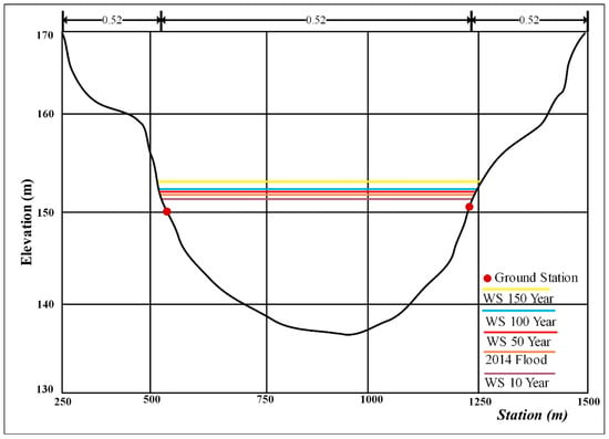
Figure 7.
Water level for floods with different return periods 1118 m downstream from Taunsa Barrage.
3.4. Flood Plain Mapping
The flooded area for floods of different return periods was delineated using the model and Figure 8 depicts the areas of the river basin expected to be flooded for a flood with a 50-year return period. Figure 9 illustrates the extent of the flood according to the model in comparison to the extent observed on the MODIS satellite image. Through visual inspection, the hydraulic model simulates very well the spatial extent of the 2014 flood. Although the timing of the satellite image does not exactly correspond with the peak flood timing, field surveys in the study area indicate that the highest flood happened around August 7. However, some positions had minor deviations, the accuracy of the floodplain geometry used in the HEC-RAS model may cause those deviations. There were several islands and reservoirs on the water surface created by ArcGIS, possibly because the DEM elevations had a 1 m interval. The surface of water assumed constant elevation values. Consequently, compared to the lower reach, the flooded area in the upper section of the river and flow depth are comparatively smaller.
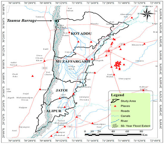
Figure 8.
Areas in the Muzaffargarh District expected to be flooded for a flood with a 50-year return period.
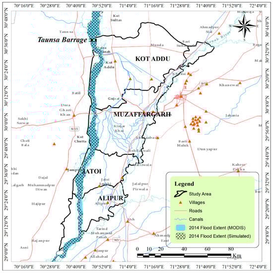
Figure 9.
Comparison of the extent of the 2014 flood according to the MODIS satellite image and the hydraulic simulation of the flood.
Near Taunsa Barrage lies the highest area impacted. It can be seen from Table 6 that for the 100-year return period, more than 147% of the surface area is expected to be flooded.
Table 6.
Percentage of the surface area flooded during floods of different return periods.
Overall, this study indicates that the accuracy of the HEC-RAS model to simulate the spatial extent of the 2014 flood of the Indus River to be very good, through visual inspection, but better calibration of the channel roughness could potentially further increase the accuracy of the model.
4. Discussion
Pakistan is a country highly vulnerable to floods [45,46]. For instance, in the past decade, other disasters were overshadowed by floods due to the heavy death toll and the significant disruption to the economy that they caused [34,47]. In 2014, heavy monsoon rains resulted in a high discharge of the Indus River, which exceeded the channel capacity, causing a major flood in Muzaffargarh District of the Punjab province.
This paper showed that a supervised classification of Landsat images was able to identify the LULC types of the study region with a high degree of accuracy. Even though Landsat images are available at a relatively high spatial resolution, they are typically available every 15 days over the study area [34], a time interval that is not frequent enough for flood monitoring and that is also often not suitable for damage assessment, especially given that cloud coverage sometimes restricts the use of optical images [48,49]. This was different for path 151 of the Landsat, which provided cloud-free images over the study area at the time of the 2014 flood, allowing for the current study to be performed.
Previous research has shown the potential of optical satellite imagery to monitor inundated farmland and built-up areas [2]. This study has further expanded this evidence to other LULC types. Moreover, the potential of using Landsat images for damage assessment, even many days following a flood, is demonstrated in this paper, a result in agreement with other studies [26,37]. This paper also shows that sediment build-up can also be detected with good accuracy over crop/agricultural fields and built-up areas [48].
When assessing the reliability of the flood monitoring reports, the precision of the satellite data and the methods used to process and analyze them must also be considered. This analysis performed in this paper has provided an accuracy of more 85% for the LULC categorization. This analysis identified ‘sand’ with an accurate accuracy, however, wet sand has often been mistaken with water and vegetation/agricultural land in some instances. This is also observed in some situations where blurred pixels, crop/agricultural land, and built-up areas are also misclassified in transition areas.
For flood mapping and damage assessment, high-resolution SAR data are suggested [50]. This is because radar satellite imagery can penetrate clouds, thereby they can be used under any weather conditions [50], and they are considered more accurate to assess disruption to crop/agricultural land and built-up areas [6,48]. However, freely available SAR images could not be obtained during the timing of the 2014 flood. Finally, in built-up areas where floodwaters flow over buildings, roads, and other elements, the modest 30 m spatial resolution of the Landsat images can lead to misclassification.
Another objective of this study was to evaluate the suitability of the HEC-RAS model to simulate the water surface profiles and determine the spatial extent of floods of different return periods. It was found that the HEC-RAS model was able to replicate the magnitude of the 2014 flood. The floodplain map showed that the flood levels were about four times higher for a flood with a 50-year return period than those under typical flow conditions. During the field surveys, it was noticed that the marginal barriers are necessary to restore, because the villagers cut them down in many places and build passages for their tractors and cattle. The deterioration of the foundations of barriers has contributed to the extent of the 2014 flood. The interference by citizens is another related concern with the protection of the floodplain in the basin. In recent years, the population and anthropogenic activities have increased in the floodplains. The floodplain must be reinstated or maintained to its natural undeveloped state to ensure citizens and infrastructure safety. Protection from damage and restoring the floodplain will significantly mitigate the risk of flooding. This paper has shown the potential of applying the HEC-RAS model in the simulation of the 2014 flood, and could be used by relevant authorities to inform risk mitigation strategies. It is cost-effective and would allow government agencies to reduce flood damage. While hydraulic models are known to be challenging to implement, several institutions in Pakistan are now familiar with the HEC-RAS model.
5. Conclusions
This study proposed a modelling approach using GIS and RS to depict the spatial extent of the 2014 flood of the Indus River in Pakistan, comparing the model output with MODIS satellite imagery, and determining the extent of floods of different return periods for the basin, in addition to assessing the damage caused by the flood. The methodology consisted of using Landsat images to identify the various LULC types over the watershed and the approach was subsequently evaluated using Google Earth images and field data with an overall classification accuracy of 85% obtained. Also, the analysis found that the ‘crop/agricultural land’ LULC type was the most affected by the flood. This research also evaluated the HEC-RAS model to simulate the 2014 flood and using the model to simulate floods of different return periods. The K-S statistical test identified the LP3 probability distribution to be best at simulating the flow regime of the Indus River at Taunsa Barrage, and this distribution was then used to identify the peak river discharge for floods with a 5-, 10-, 50-, 100-, and 150-year return period, which was then used as input into the HEC-RAC model to estimate the areas of the watershed at risk of flooding for each return period. The spatial extent of the 2014 flood, as simulated by the model, was found to agree very well with the extent of the flood as observed on a MODIS satellite image, showing the potential of using the model and the approach presented in this paper for risk mitigation.
Author Contributions
A.T.: conceptualization, writing—review and editing, methodology, software, formal analysis, visualization, data curation, writing—original draft, investigation, validation; H.S.: supervision, visualization, validation, investigation, writing—review and editing; A.K.: visualization, validation, investigation, writing—review and editing, supervision; S.S.: writing—review and editing; A.S.G.: investigation, writing—review and editing; L.L.: investigation, writing—review and editing; N.T.T.L.: writing—review and editing, project management; Q.B.P.: visualization, validation, investigation, supervision, writing—review and editing. All authors have read and agreed to the published version of the manuscript.
Funding
No external funding.
Data Availability Statement
The data presented in this study are available on request from the first or corresponding authors.
Acknowledgments
We are thankful to Shazada Adnan from the Pakistan Meteorological Department in Islamabad, who provided the flood data necessary for this research. We also thank Liping Zhang, Head of State Key Laboratory of Hydrology at Wuhan University, China, for his support at various stages of the analysis and writing. Finally, we acknowledge the three anonymous reviewers and editors of the special issue of the journal who provided very helpful comments that helped improved the final version of the manuscript.
Conflicts of Interest
The authors declare no conflict of interest.
References
- Islam, R.; Kamaruddin, R.; Ahmad, S.A.; Jan, S.J.; Anuar, A.R. A review on mechanism of flood disaster management in Asia. Int. Rev. Manag. Mark. 2016, 6, 1. [Google Scholar]
- Khan, B.; Iqbal, M.J.; Yosufzai, M.A.K. Flood risk assessment of River Indus of Pakistan. Arab. J. Geosci. 2010, 4, 115–122. [Google Scholar] [CrossRef]
- Asad Sarwar, Q. Water management in the Indus Basin in Pakistan: Challenges and opportunities. Mt. Res. Dev. 2011, 31, 252–260. [Google Scholar]
- Ullah, I.; Ma, X.; Yin, J.; Asfaw, T.G.; Azam, K.; Syed, S.; Liu, M.; Arshad, M.; Shahzaman, M. Evaluating the meteorological drought characteristics over Pakistan using in situ observations and reanalysis products. Int. J. Clim. 2021. [Google Scholar] [CrossRef]
- D’Addabbo, A.; Refice, A.; Pasquariell, G.; Lovergine, F.P.; Capolongo, C.; Manfreda, S. A Bayesian network for flood detection combining SAR imagery and ancillary data. IEEE Trans. Geosci. Remote Sens. 2016, 54, 3612–3625. [Google Scholar] [CrossRef]
- Sanyal, J.; Lu, X.X. Application of remote sensing in flood management with special reference to Monsoon Asia: A review. Nat. Hazards 2004, 33, 283–301. [Google Scholar] [CrossRef]
- Chaudhry, Z.A. Hydraulic/structural deficiencies at the Taunsa Barrage. Pak. J. Sci. 2009, 61, 135–140. [Google Scholar]
- Quirós, E.; Gagnon, A.S. Validation of flood risk maps using open source optical and radar satellite imagery. Trans. GIS 2020, 24, 1208–1226. [Google Scholar] [CrossRef]
- Julzarika, A.; Harintaka. Indonesian DEMNAS: DSM or DTM? In Proceedings of the 2019 IEEE Asia-Pacific Conference on Geoscience, Electronics and Remote Sensing Technology (AGERS), Jakarta, Indonesia, 26–27 August 2019; pp. 31–36. [Google Scholar]
- Florinsky, I.V. Chapter 3—Digital elevation models. In Digital Terrain Analysis in Soil Science and Geology, 2nd ed.; Florinsky, I.V., Ed.; Academic Press: Cambridge, MA, USA, 2016; pp. 77–108. [Google Scholar] [CrossRef]
- Wang, Y.; Chen, A.S.; Fu, G.; Djordjević, S.; Zhang, C.; Savić, D.A. An integrated framework for high-resolution urban flood modelling considering multiple information sources and urban features. Environ. Model. Softw. 2018, 107, 85–95. [Google Scholar] [CrossRef]
- Shafapour Tehrany, M.; Shabani, F.; Neamah Jebur, M.; Hong, H.; Chen, W.; Xie, X. GIS-based spatial prediction of flood prone areas using standalone frequency ratio, logistic regression, weight of evidence and their ensemble techniques. Geomat. Nat. Hazards Risk 2017, 8, 1538–1561. [Google Scholar] [CrossRef]
- Gashaw, W.; Legesse, D. Flood hazard and risk assessment using GIS and remote sensing in fogera woreda, Northwest Ethiopia. In Nile River Basin: Hydrology, Climate and Water Use; Melesse, A.M., Ed.; Springer: Dordrecht, The Netherlands, 2011; pp. 179–206. [Google Scholar] [CrossRef]
- Elkhrachy, I. Flash flood hazard mapping using satellite images and GIS tools: A case study of Najran City, Kingdom of Saudi Arabia (KSA). Egypt. J. Remote Sens. Space Sci. 2015, 18, 261–278. [Google Scholar] [CrossRef]
- Samanta, S.; Pal, D.K.; Palsamanta, B. Flood susceptibility analysis through remote sensing, GIS and frequency ratio model. Appl. Water Sci. 2018, 8, 66. [Google Scholar] [CrossRef]
- Syifa, M.; Park, S.J.; Achmad, A.R.; Lee, C.-W.; Eom, J. Flood mapping using remote sensing imagery and artificial intelligence techniques. A case study in Brumadinho, Brazil. J. Coast. Res. 2019, 90, 197–204. [Google Scholar] [CrossRef]
- Ahamed, A.; Bolten, J.; Doyle, C.; Fayne, J. Near real-time flood monitoring and impact assessment systems. In Remote Sensing of Hydrological Extremes; Lakshmi, V., Ed.; Springer International Publishing: Cham, Switzerland, 2017; pp. 105–118. [Google Scholar] [CrossRef]
- Rahman, M.S.; Di, L. A systematic review on case studies of remote-sensing-based flood crop loss assessment. Agriculture 2020, 10, 131. [Google Scholar] [CrossRef]
- Di, L.; Yu, E.G.; Kang, L.; Shrestha, R.; Bai, Y.-Q. RF-CLASS: A remote-sensing-based flood crop loss assessment cyber-service system for supporting crop statistics and insurance decision-making. J. Integr. Agric. 2017, 16, 408–423. [Google Scholar] [CrossRef]
- Chow, M.F.; Yusop, Z.; Toriman, M.E. Modelling runoff quantity and quality in tropical urban catchments using Storm Water Management Model. Int. J. Environ. Sci. Technol. 2012, 9, 737–748. [Google Scholar] [CrossRef]
- Rahman, G.; Rahman, A.-U.; Anwar, M.; Khan, M.; Ashraf, H.; Zafar, U. Socio-economic damages caused by the 2014 flood in Punjab province, Pakistan. Proc. Pak. Acad. Sci. 2017, 54, 365–374. [Google Scholar]
- Sajjad, A.; Lu, J.; Chen, X.; Chisenga, C.; Saleem, N.; Hassan, H. Operational monitoring and damage assessment of riverine flood-2014 in the lower Chenab plain, Punjab, Pakistan, using remote sensing and GIS techniques. Remote Sens. 2020, 12, 714. [Google Scholar] [CrossRef]
- Hussain, M.; Butt, A.R.; Uzma, F.; Ahmed, R.; Irshad, S.; Rehman, A.; Yousaf, B. A comprehensive review of climate change impacts, adaptation, and mitigation on environmental and natural calamities in Pakistan. Environ. Monit. Assess. 2019, 192, 48. [Google Scholar] [CrossRef]
- Abedin, S.; Stephen, H. GIS framework for spatiotemporal mapping of urban flooding. Geosciences 2019, 9, 77. [Google Scholar] [CrossRef]
- Das, S.; Patel, P.P.; Sengupta, S. Evaluation of different digital elevation models for analyzing drainage morphometric parameters in a mountainous terrain: A case study of the Supin-Upper Tons Basin, Indian Himalayas. Springerplus 2016, 5, 1544. [Google Scholar] [CrossRef] [PubMed]
- Towfiqul Islam, A.R.M.; Talukdar, S.; Mahato, S.; Kundu, S.; Eibek, K.U.; Pham, Q.B.; Kuriqi, A.; Linh, N.T.T. Flood susceptibility modelling using advanced ensemble machine learning models. Geosci. Front. 2021, 12. in press. [Google Scholar] [CrossRef]
- Mahmood, S.; Rahman, A.-u.; Sajjad, A. Assessment of 2010 flood disaster causes and damages in district Muzaffargarh, Central Indus Basin, Pakistan. Environ. Earth Sci. 2019, 78, 63. [Google Scholar] [CrossRef]
- Yerramilli, S. A hybrid approach of integrating HEC-RAS and GIS towards the identification and assessment of flood risk vulnerability in the city of Jackson, MS. Am. J. Geogr. Inf. Syst. 2012, 1, 7–16. [Google Scholar] [CrossRef]
- Demir, V.; Kisi, O. Flood hazard mapping by using geographic information system and hydraulic model: Mert River, Samsun, Turkey. Adv. Meteorol. 2016, 2016, 1–9. [Google Scholar] [CrossRef]
- Gorokhovich, Y.; Voustianiouk, A. Accuracy assessment of the processed SRTM-based elevation data by CGIAR using field data from USA and Thailand and its relation to the terrain characteristics. Remote Sens. Environ. 2006, 104, 409–415. [Google Scholar] [CrossRef]
- Sanders, B.F. Evaluation of on-line DEMs for flood inundation modeling. Adv. Water Resour. 2007, 30, 1831–1843. [Google Scholar] [CrossRef]
- Khattak, M.S.; Anwar, F.; Saeed, T.U.; Sharif, M.; Sheraz, K.; Ahmed, A. Floodplain mapping using HEC-RAS and ArcGIS: A case study of Kabul River. Arab. J. Sci. Eng. 2015, 41, 1375–1390. [Google Scholar] [CrossRef]
- Khalil, U.; Muhammad Khan, N.; Rehman, H. Floodplain mapping for Indus River: Chashma–Taunsa Reach. Pak. J. Eng. Appl. Sci. 2017, 20, 30–48. [Google Scholar]
- Khalid, B.; Cholaw, B.; Alvim, D.S.; Javeed, S.; Khan, J.A.; Javed, M.A.; Khan, A.H. Riverine flood assessment in Jhang district in connection with ENSO and summer monsoon rainfall over Upper Indus Basin for 2010. Nat. Hazards 2018, 92, 971–993. [Google Scholar] [CrossRef]
- Chohan, K.; Ahmad, S.R.; ul Islam, Z.; Adrees, M. Riverine flood damage assessment of cultivated lands along Chenab River using GIS and remotely sensed data: A case study of district Hafizabad, Punjab, Pakistan. J. Geogr. Inf. Syst. 2015, 7, 506–526. [Google Scholar] [CrossRef]
- Chignell, S.; Anderson, R.; Evangelista, P.; Laituri, M.; Merritt, D. Multi-temporal independent component analysis and landsat 8 for delineating maximum extent of the 2013 Colorado front range flood. Remote Sens. 2015, 7, 9822–9843. [Google Scholar] [CrossRef]
- Rokni, K.; Ahmad, A.; Selamat, A.; Hazini, S. Water feature extraction and change detection using multitemporal landsat imagery. Remote Sens. 2014, 6, 4173–4189. [Google Scholar] [CrossRef]
- Vogel, R.M.; Thomas, W.O.; McMahon, T.A. Flood-flow frequency model selection in southwestern United States. J. Water Resour. Plan. Manag. 1993, 119, 353–366. [Google Scholar] [CrossRef]
- Frangopol, D.M. Probability concepts in engineering: Emphasis on applications to civil and environmental engineering. Struct. Infrastruct. Eng. 2008, 4, 413–414. [Google Scholar] [CrossRef]
- Katz, R.W.; Parlange, M.B.; Naveau, P. Statistics of extremes in hydrology. Adv. Water Resour. 2002, 25, 1287–1304. [Google Scholar] [CrossRef]
- Wang, Q.J. LH moments for statistical analysis of extreme events. Water Resour. Res. 1997, 33, 2841–2848. [Google Scholar] [CrossRef]
- Hoshi, K.; Stedinger, J.R.; Burges, S.J. Estimation of log-normal quantiles: Monte Carlo results and first-order approximations. J. Hydrol. 1984, 71, 1–30. [Google Scholar] [CrossRef]
- McCuen, R. Microcomputer Applications in Statistical Hydrology; Prentice Hall: Hoboken, NJ, USA, 1992. [Google Scholar]
- Sañudo, E.; Cea, L.; Puertas, J. Modelling pluvial flooding in urban areas coupling the models iber and SWMM. Water 2020, 12, 2647. [Google Scholar] [CrossRef]
- Siddiqui, M.J.; Haider, S.; Gabriel, H.F.; Shahzad, A. Rainfall–runoff, flood inundation and sensitivity analysis of the 2014 Pakistan flood in the Jhelum and Chenab river basin. Hydrol. Sci. J. 2018, 63, 1976–1997. [Google Scholar] [CrossRef]
- Mahmood, S.; Khan, A.-u.-H.; Mayo, S.M. Exploring underlying causes and assessing damages of 2010 flash flood in the upper zone of Panjkora River. Nat. Hazards 2016, 83, 1213–1227. [Google Scholar] [CrossRef]
- Azar, D.; Engstrom, R.; Graesser, J.; Comenetz, J. Generation of fine-scale population layers using multi-resolution satellite imagery and geospatial data. Remote Sens. Environ. 2013, 130, 219–232. [Google Scholar] [CrossRef]
- Musa, Z.N.; Popescu, I.; Mynett, A. A review of applications of satellite SAR, optical, altimetry and DEM data for surface water modelling, mapping and parameter estimation. Hydrol. Earth Syst. Sci. 2015, 19, 3755. [Google Scholar] [CrossRef]
- Qi, S.; Brown, D.G.; Tian, Q.; Jiang, L.; Zhao, T.; Bergen, K.M. Inundation extent and flood frequency mapping using LANDSAT imagery and digital elevation models. GISci. Remote Sens. 2013, 46, 101–127. [Google Scholar] [CrossRef]
- Giordan, D.; Notti, D.; Villa, A.; Zucca, F.; Calò, F.; Pepe, A.; Dutto, F.; Pari, P.; Baldo, M.; Allasia, P. Low cost, multiscale and multi-sensor application for flooded area mapping. Nat. Hazards Earth Syst. Sci. 2018, 18, 1493–1516. [Google Scholar] [CrossRef]


Publisher’s Note: MDPI stays neutral with regard to jurisdictional claims in published maps and institutional affiliations. |
© 2021 by the authors. Licensee MDPI, Basel, Switzerland. This article is an open access article distributed under the terms and conditions of the Creative Commons Attribution (CC BY) license (https://creativecommons.org/licenses/by/4.0/).