Plot-Based Classification of Macronutrient Levels in Oil Palm Trees with Landsat-8 Images and Machine Learning

Abstract

Oil palm crops are essential for ensuring sustainable edible oil production, in which production is highly dependent on fertilizer applications. Using Landsat-8 imageries, the feasibility of macronutrient level classification with Machine Learning (ML) was studied. Variable rates of compost and inorganic fertilizer were applied to experimental plots and the following nutrients were studied: nitrogen (N), phosphorus (P), potassium (K), magnesium (Mg) and calcium (Ca). By applying image filters, separability metrics, vegetation indices (VI) and feature selection, spectral features for each plot were acquired and used with ML models to classify macronutrient levels of palm stands from chemical foliar analysis of their 17th frond. The models were calibrated and validated with 30 repetitions, with the best mean overall accuracy reported for N and K at 79.7 ± 4.3% and 76.6 ± 4.1% respectively, while accuracies for P, Mg and Ca could not be accurately classified due to the limitations of the dataset used. The study highlighted the effectiveness of separability metrics in quantifying class separability, the importance of indices for N and K level classification, and the effects of filter and feature selection on model performance, as well as concluding RF or SVM models for excessive N and K level detection. Future improvements should focus on further model validation and the use of higher-resolution imaging.

1. Introduction

The global population is projected to reach 7.58 billion by the end of the year and an additional 27.7 million tonnes of edible oil will be required to fulfill food demands. With its greater per-hectare production and economic competitiveness, oil palm is a pivotal crop in ensuring sufficient edible oil is available in the global market [1]. Agriculture has at times become a controversial topic among conservationists due to its negative impacts on the environment, such as biodiversity loss, deforestation, and increased carbon emissions [2,3,4,5]. Precision agriculture (PA), which involves informed decision making in agriculture using information interpreted from sensor-based data (such as the remote sensing data in this paper) or other sources, is currently sought as a solution for improved sustainable food production [6,7,8,9].

In fertilizer application, PA enables site specific management by determining macronutrient status and fertilizer requirement in individual plants. These macronutrients include nitrogen (N), phosphorus (P), potassium (K), magnesium (Mg) and calcium (Ca), which are essential for ensuring good plant health [7,8,9,10]. Like most plants, macronutrient levels in palm trees are diagnosed via removal of leaflets for destructive chemical analysis, such as the Kjeldahl method for N determination [11,12,13,14,15,16,17,18,19,20,21,22,23]. By relating remote sensing and GIS technology data with field results at promising accuracy and precision, the findings could be extrapolated to plantation scales, enabling more efficient, economic and non-destructive means of fertilizer management. This ensures global food security is met under sustainable terms via increasing crop production with available land and resource [7,8,15,20].

Spectroradiometers are the fundamental sensing tools utilized in nutrient prediction, due to their capacity to record reflectance readings ranging from the visible (VIS) to the shortwave infrared (SWIR) region of the electromagnetic spectrum (300–2500 nm) in hundreds of narrow wavebands. The data heaps from spectroradiometers warranted the use of machine learning (ML) subsequently, due to its ability to extract information from datasets with high dimensions and non-linear structures [20,21,22]. Because ML algorithms acquire their solutions with different mathematical approaches, this prompts the adoption of at least two algorithms in most studies for comparison purposes [18,19,20,21,22]. Successful predictions with spectroradiometer data have been seen in rice [18,23,24,25,26], citrus [11,12], wheat [10,20,27,28,29], oilseed rape [13,16,30], pastures [21,22,31,32,33] and other plants [34,35,36].

It can be seen that the wavelengths selected in literature for N prediction are focused in the green (i.e., 510–550 nm) and red edge (i.e., 710–750 nm) regions, which correspond to chlorophyll characteristics [12,20,37]; this is contrary to P and K, in which wavelengths at the SWIR region play a large role, in addition to those in the VISNIR region [13,14,23,29,30,32,33,34,35]. Additionally, specific wavelengths identified as significant explanatory variables may be used to derive vegetation indices (VI) mathematically for improved prediction [23,29]. However, the exact wavelengths identified for predictions may differ between crops, their varieties, and methods used. The authors of [20] identified 526 nm and 716 nm as ideal predictors for wheat N, while [25] concluded 522 nm and 740 nm for rice N, with both studies using the ratio of the readings from the first derivatives of their respective wavelength pairs. On the other hand, [13,30] identified several highly similar wavelengths despite use of different methods for oil seed rape N prediction ([13]: 513 nm, 542 nm, 718 nm, 928 nm, 1015 nm; [30]: 574 nm, 719 nm, 918 nm, 1017 nm).

It remains unfortunate that spectroradiometers are unaffordable for most agricultural practitioners, in addition to its more laborious nature when plants have to be scanned individually for plantation-scale monitoring. Multispectral imaging from satellite sensors may offer a solution to wide-scale and affordable measures for nutrient monitoring. To date, a handful of research has attempted N prediction using high spatial resolution (<5 m) multispectral images captured from commercial satellites, such as QuickBird [38], GeoEye-1 [39], SPOT 7 [40] and WorldView-2 [41], with promising results. Sadly, free medium-resolution data from satellite sensors such as Landsat-8 OLI, Sentinel 2 MSI, ASTER and Sentinel 3 OLCI were even greater in rarity [42,43], or at best, simulated with spectroradiometer readings [31]. In palm trees, similar platforms (i.e., spectroradiometer and high resolution images) have been explored for the prediction of N, P and K [40,44,45,46], although difficulty in its widespread application still remains with its inaccessibility to oil palm smallholders.

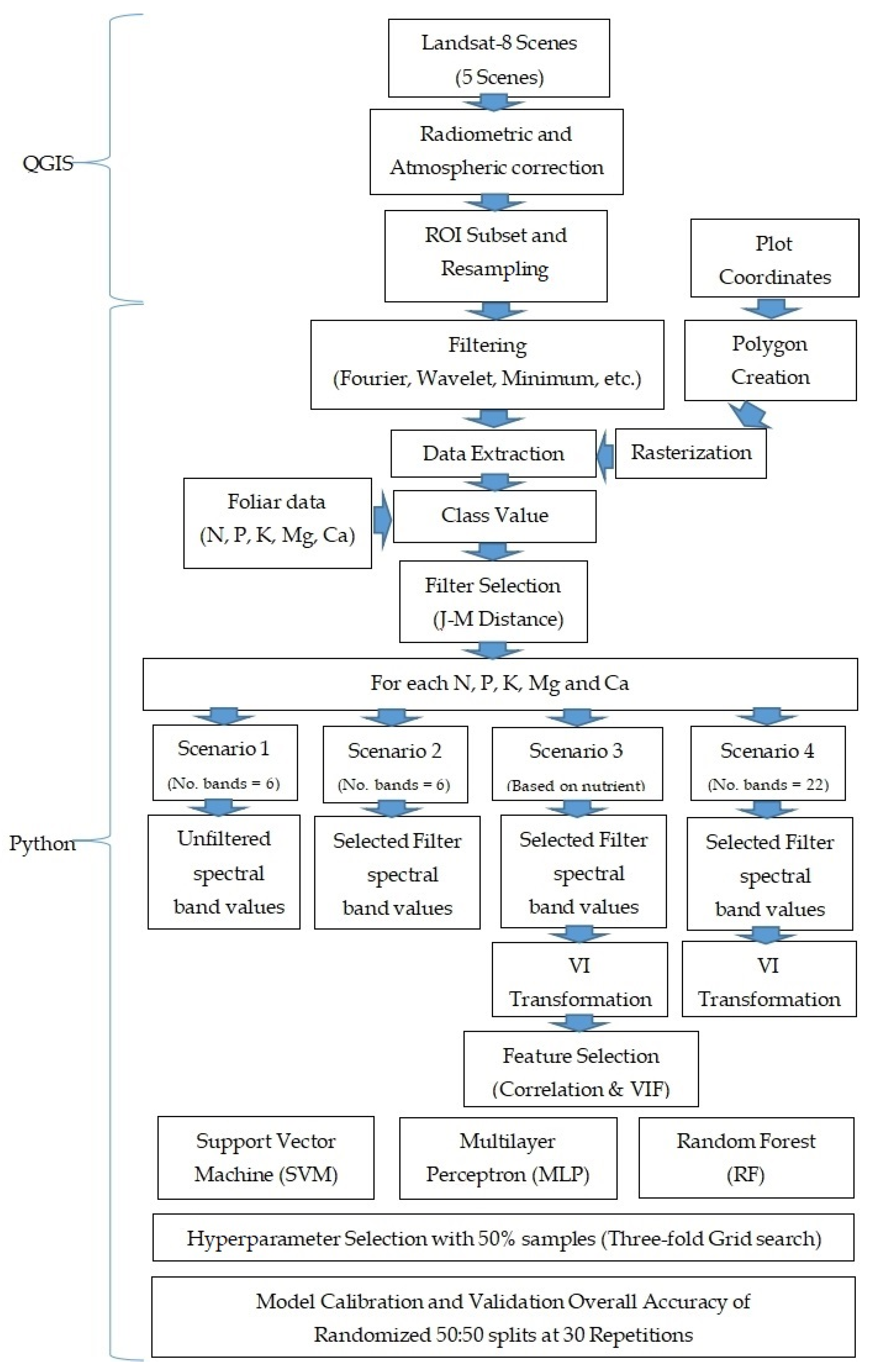
Taking leverage of its free availability and consistent revisit frequency, this study assessed Landsat-8 OLI satellite imageries and ML algorithms (i.e., Support Vector Machine (SVM), Artificial Neural Network (ANN), Random Forest (RF)) in classifying nutrient levels of palm trees with different treatments for the following macronutrients: nitrogen (N), phosphorus (P), potassium (K), magnesium (Mg) and calcium (Ca). Given its 30 m resolution, the study proposed an open-source and plot-based method to classify the nutrient status of palm trees via image processing, feature extraction and ML classification. The aim of this study is to produce a freely available nutrient level classification model with Landsat-8 OLI imageries as input. Studies to date on nutrient estimation have only focused on spectroradiometer data or high resolution imaging, particularly for N. The positive results acquired from this research will open insights to the potential of using easily available coarse satellite imaging in classifying plot N and other macronutrient levels via ML, subsequently allowing long-term monitoring of palm plantations at a large scale. This would not only promote efficient, convenient and cost-effective nutrient management at a plantation scale, but increase the accessibility of nutrient monitoring to smallholders.

2. Materials and Methods

2.1. Study Area and Experimental Setup

The study was carried out at an oil palm plantation located in Johor, Malaysia, from 2013 to 2017 (Figure 1). The palm trees were planted at a 144 trees/hectare (ha) density. Malaysia is a country with a tropical climate due to its proximity to the equator. According to [47,48], the study area is characterized by lowlands consisting of soil from the Rengam series (USDA Soil Taxonomy: Ultisols). Temperature, average monthly rainfall and average wind speed in the area during the study period ranged from 23 °C to 33 °C (annual average: 29 °C), 64.01 mm to 350.9 mm (annual average: 2066.4 mm) and 3.9 to 9.7 km/h, respectively [49]. Overall, soil and climate conditions were suitable for palm cultivation with possible improvements from fertilizer application [48,50]. In total, the experimental plots covered 3.97 ha of palm trees, spanning across 39.44 ha of palm plantation. Palm stands were aged five and half years when the experiment was initially conducted. Three levels of inorganic fertilizer and four levels of compost were applied for N, P, K and Mg in a factorial design with three replicates for each tree. N, P, K and Mg fertilizers applied were ammonium chloride (NH₄Cl), rock phosphate (P), muriate of potash (KCl) and kieserite (MgSO₄·H₂O). This resulted in 36 plot observations in total. Specific details on treatment levels are shown in

Table 1. Description of fertilizer and compost treatment levels for nitrogen (N), phosphorus (P), potassium (K) and magnesium (Mg). Amounts are measured in kg nutrient per tree.

Treatment Levels	Fertilizer Treatment (N, P, K, Mg in kg palm−1 year−1)	Compost Treatment (N, P, K, Mg in kg palm−1 year−1)
1	0, 0, 0, 0	0, 0, 0, 0
2	0.42, 0.53, 0.60, 0.16	0.45, 0.13, 0.80, 0.12
3	0.84, 1.05, 1.20, 0.34	0.90, 0.26, 1.60, 0.24
4	N/A	1.35, 0.40, 2.40, 0.36

and Figure 1. It should be noted that soil and plant interactions were not taken into account in this study as this research’s purpose is to evaluate the potential of ML models in classifying nutrient levels in palm tree plots using coarse imagery, and fertilizer applications were conducted to induce nutrient level variability in plots.

2.2. Materials/Data Collection

Each plot consisted of 4 × 3 (12) palm trees, with an average plot area of 1100 m². In each plot, frond 17 from all 12 palm trees was sampled to produce ground truth by destructive foliar analysis and its nutrient status was acquired as a mean of all observations in the plot. Frond 17 was selected as the reference for palm tree nutrient levels due to past studies indicating its greater representation of nutrient status and correlation between nutrient contents and yield [51]. N was acquired using combustion or near-infrared (NIR) spectroscopy, while P, K, Mg and Ca were acquired by wet ashing or NIR spectroscopy [52]. The acquired foliar nutrient status was reported in % dry matter (DM). By conducting the experiment for five consecutive years (2013–2017), 36 plot observations from each year yielded 180 samples in total. The coordinates of the four corners of each plot (Figure 1) were recorded using a Trimble Geo7 handheld GPS device.

For image acquisition, Landsat-8 OLI/TIRS imageries (Level 1 Product) were downloaded from the Earth Explorer-USGS website (earthexplorer.usgs.gov, accessed on 15 December 2020). Launched in 2013, the Landsat-8 satellite is mounted with the Operational Land Imager (OLI) and the Thermal Infrared Sensor (TIRS) instrument, offering images scenes with nine spectral bands (aerosol: 0.43–0.45 μm; blue (B): 0.45–0.51 μm; green (G): 0.53–0.59 μm; red (R): 0.64–0.67 μm; near-infrared (NIR): 0.85–0.88 μm; shortwave infrared 1 (SWIR1): 1.57–1.65 μm; shortwave infrared 2 (SWIR2): 2.11–2.29 μm; panchromatic (Pan): 0.50–0.68 μm; cirrus (Cir): 1.36–1.38 μm) and two thermal bands (thermal infrared 1 (TIR1): 10.6–11.19 μm; thermal infrared 2 (TIR2): 11.5–12.51 μm), at 30 m (panchromatic at 15 m) and 100 m spatial resolution respectively. Images close to sampling dates were manually screened to ensure the subset consisting of the study site was cloud-free, followed by further inspection with the quality assessment band (BQA) provided in the download. Overall, the selected images were +/− 2 weeks from the stipulated date. Specific details of selected imageries are as below (

Table 2. Date of foliar sampling in each year and description of Landsat-8 OLI/TIRS images selected for analysis.

Year	Foliar Sampling Period	Image_Date	Path	Row
2013	4/2013	24 April 2013	125	59
2014	4/2014	26 March 2014	125	59
2015	10/2015	7 October 2015	125	59
2016	10/2016	10 November 2016	125	59
2017	10/2017	26 September 2017	125	59

).

2.3. Methods

2.3.1. Data Processing

QGIS and the Python programming language were used for all data processing in the study. Nutrient level classes were constructed based on critical value ranges provided by [53] (See Appendix A.3,

Table A1. Critical values for nutrient levels in leaf 17 of palm stands aged more than 6 years from planting (Source: [52]).

	N	P	K	Mg	Ca
Units	%DM	%DM	%DM	%DM	%DM
Deficient	x < 2.30	x < 0.14	x < 0.75	x < 0.20	x < 0.25
Margin Def	2.30 ≤ x < 2.40	0.14 ≤ x < 0.15	0.75 ≤ x < 0.90	0.20 ≤ x < 0.25	0.25 ≤ x < 0.50
Optimum	2.40 ≤ x ≤ 2.80	0.15 ≤ x≤ 0.18	0.90 ≤ x ≤ 1.20	0.25 ≤ x ≤ 0.40	0.50 ≤ x ≤ 0.75
Margin Ex	2.80 < x ≤ 3.00	0.18 < x ≤ 0.25	1.20 < x ≤ 1.60	0.40 < x ≤ 0.70	0.75 < x ≤ 1.00
Excessive	x > 3.00	x > 0.25	x > 1.60	x > 0.70	x > 1.00

). As a result, five class ranges were produced and assigned with an ordinal class value: Deficient = 1, Marginally Deficient = 2, Optimum = 3, Marginally Excessive = 4 and Excessive = 5. For each nutrient observation of each plot, its value is therefore assigned based on the derived class ranges (e.g., a plot observation of 2.50% N in DM would be in the Optimum class range and thus assigned the class value 3). The distribution of samples among nutrient levels is shown in

Table 3. Distribution of observations based on critical values of nutrient levels before (Left) and after (Right) merging low sample classes.

	Initial Distribution					Corrected Distribution
Class	N	P	K	Mg	Ca	N	P	K	Mg	Ca
Deficient (Def)	0	0	0	2	0	0	0	0	0	0
Margin Def (Mar Def)	0	8	0	76	2	0	0	0	78	0
Optimum (Opt)	62	163	68	99	154	62	177	68	99	156
Margin Ex (Mar Ex)	94	6	109	0	21	94	0	109	0	21
Excessive (Ex)	21	0	0	0	0	21	0	0	0	0

(Left). To reduce overfitting or biased analysis, observations from nutrient level classes identified to have less than 10 samples are merged with the adjacent class, yielding Table 3 (Right).

The best image scene identified each year was atmospherically corrected by applying a Dark Object Subtraction (i.e., DOS1) algorithm from a plugin in QGIS by [54]. Despite the availability of Landsat-8 Surface Reflectance images (Level-2 Product) provided by USGS, the study proceeded with DOS due the transferrability of the approach between images from different platforms. This approach would enable a transferrable model to be developed in events where surface reflectance products are not available for a particular image and simple atmospheric correction without cost and climatological parameters are required. Using GoogleEarth Pro as reference, the series of satellite images was checked for co-registration, followed by a subset and resampling with the nearest neighbour to produce a Region of Interest (ROI). In a shapefile layer, the recorded coordinates for the four corners of each plot were used to produce a rectangular polygon feature encompassing the plot area. The shapefile layer was rasterized to produce a binary mask with a dimension equal to the ROI (294 × 524 pixels) as means to extract the band mean reflectance values of all plots in the ROI (Appendix A.1, Figure A1). The spatial resolution of the resampled ROI and the binary mask was determined at 1.6 m as the resolution required to preserve the rectangular shape of the polygon features during rasterization. It was essential to ensure a suitable resampling resolution was selected based on the size of polygons as a low resampling resolution would result in overestimation of polygon area and incorrect value extraction [55,56,57] (See Figure A2 and Figure A3 at Appendix A.1). Masking and extraction enabled only mean values calculated from the extent of each plot in the ROI to be included in further analysis. The acquisition of these values allowed subsequent calculation of the Jeffries–Matusita (J-M) distance for all possible pairwise combinations of nutrient levels in each nutrient to quantify the separability of values between plots from different nutrient levels. The J-M distance is a distance which takes into account the covariance matrix between features of pairwise classes (Equation (1)). The value ranges from 0 to 2, with a value >1.8 between classes considered good for separability [54,58,59,60]:

$$\begin{gathered} B=\frac{1}{8}{(x-y)}^t{\left(\frac{{\displaystyle \sum x}+{\displaystyle \sum y}}{2}\right)}^{-1}(x-y)+\frac{1}{2}\ln \left(\frac{\left|\frac{{\displaystyle \sum x}+{\displaystyle \sum y}}{2}\right|}{{\left|{\displaystyle \sum x}\right|}^{\frac{1}{2}}{\left|{\displaystyle \sum y}\right|}^{\frac{1}{2}}}\right), \\ {J}_{xy}=2\left(1-e^{-B}\right) \end{gathered}$$

(1)

where:

• x, y = first and second spectral signature vector
• ${\displaystyle \sum x}$, ${\displaystyle \sum y}$ = covariance matrix of plot
• B = Bhattacharya distance
• $J_{xy}$ = Jeffries–Matusita distance

In attempts to reduce image noise and improve separability, the following filters and transforms were applied to the series of images: standard filters (i.e., min, median, max, gaussian and rank) and fast fourier transform (FFT). The process was carried out using Numpy, Pywt and Scipy libraries in Python. For FFT filtering, the image was transformed to the 2D frequency domain and swapped for quadrants to obtain the image center [61]. Values for coordinates within 1 x or y unit from the centre of domain (i.e., (0, 0), (0, 1), (1, 0), (0, −1), (−1, 0)) were retained, while other values in higher frequencies were suppressed by 10 times by multiplying the values by a coefficient of 0.1. Therefore, the filter functions as a minimum filter with the ability to suppress values at specific frequencies via the 2D frequency domain (Appendix A.2, Figure A4). To identify the best-performing filter, value extraction and distance calculation were repeated for all unfiltered (as control) and filtered image scenes, whereby the approach yielding the highest J-M distance averaged from all five nutrients was considered the best choice.

2.3.2. Vegetation Index and Feature Selection

Vegetation indices (VI) are effective in enhancing signals from vegetation and suppressing unintended noises. VIs were selected for this study by evaluating VIs listed in a review on VI development [62]. The corresponding research article where each VI was first mentioned was studied to identify its feasibility for application, with the following criteria in mind, and with priority in descending order:

• Criterion 1: VI was derived with strong theoretical or mathematical foundation
• Criterion 2: VI was derived with general applicability in mind
• Criterion 3: VI was derived with satellite bands or broadband wavelengths

In total, 16 VIs were shortlisted for application in this study, in which their respective derivation was carried using values from four bands (i.e., B, G, R and NIR) of the best filtered image. In addition to the initial bands (i.e., B, G, R, NIR, SWIR1, SWIR2), a total of 22 spectral features would be used as model inputs for nutrient level classification. The reference, index name and formula of each VI are portrayed in the table below (

Table 4. Vegetation indices (VI) selected as additional feature and for analysis. Parenthesis after full name of VI refers to acronym used throughout study.

Reference	VI	Formula
[63]	Normalized Difference Vegetation Index (NDVI)	$\frac{NIR-R}{NIR+R}$
[63]	Transformed Vegetation Index (TVI)	$\sqrt{R+0.5}$
[64]	Soil-Adjusted Vegetation Index (SAVI)	$\frac{NIR-R}{NIR+R+L}\times (1+L) L=0.5$
[65]	Green NDVI (GNDVI)	$\frac{NIR-G}{NIR+G}$
[65]	Green Atmospherically Resistant vegetation Index (GARI)	$\frac{NIR-(G-\lambda (B-R))}{NIR+(G-\lambda (B-R))} \lambda =1$
[66]	NIR/R ratio	$\frac{NIR}{R}$
[66]	NIR/G ratio	$\frac{NIR}{G}$
[67]	Soil adjusted and Atmospherically Resistant Vegetation Index (SARVI)	$\begin{array}{l}\frac{NIR-(R-\gamma (B-R))}{NIR+(R-\gamma (B-R))+L}\\ L=0.5,\gamma =1\end{array}$
[68]	Enhanced Vegetation Index (EVI)	$\begin{array}{l}Gain\frac{NIR-R}{NIR+(C1\times R)-(C2\times B)+L}\\ \mathrm{L}=1,\mathrm{C}1=6,C2=7.5,Gain=2.5\end{array}$
[69]	Atmospherically Resistance Vegetation Index (ARVI)	$\frac{NIR-(R-\gamma (B-R))}{NIR+(R-\gamma (B-R))} \gamma =1$
[70]	Modified SAVI (MSAVI)	$\frac{2NIR+1-\sqrt{{(2NIR+1)}^2-8(NIR-R)}}{2}$
[71]	Optimized SAVI (OSAVI)	$\frac{NIR-R}{NIR+R+0.16}$
[72]	Modified Simple Ratio (MSR)	$\frac{NIR}{R}-1/\sqrt{\frac{NIR}{R}+1}$
[73]	Renormalized Difference Vegetation Index (RDVI)	$\frac{NIR-R}{\sqrt{NIR+R}}$
[74]	Infrared Percentage Vegetation Index (IPVI)	$\frac{NIR}{NIR+R}$
[75]	2-Band EVI (EVI2)	$2.5\frac{NIR-R}{N+2.4R+1}$

):

VIs will be applied in two of the studied scenarios. As the VIs selected are derived from mostly similar initial bands (e.g., RDVI and IPVI both use values from R and NIR band), multicollinearity problems may occur. To address this, feature selection via correlation analysis and variance inflation factor (VIF) was conducted for one of the scenarios (i.e., Scenario 3, see Section 2.3.4). VIF has been applied in many studies involving multiple variable regressions to ensure minimal collinearity between independent variables [76,77,78]:

$$\mathrm{VIF}=\frac{1}{1-{\mathrm{R}\prime }^2}$$

(2)

where:

• R′² = coefficient of determination between an independent variable and the other independent variables.

For each nutrient, the first 11 indices with the highest correlation coefficient were selected. VIF was applied to reduce the number of features further for dimension reduction and avoiding multicollinearity problems. VIFs between the variables were generated and the six variables with the lowest VIFs were selected. It is suggested that the VIF value for each variable should be less than 10 to avoid multicollinearity. To achieve this, the calculation of VIF values for variables with each other and the elimination of the variable with the highest VIF value were conducted iteratively until all variables possessed a VIF value of less than 10 upon VIF re-calculation.

In a nutshell, processing images via Section 2.3.1 and Section 2.3.2 subsequently resulted in specific vector features with paired class values for each nutrient or scenario, which would be applied as inputs for the algorithms of interest.

2.3.3. Machine Learning

Supervised machine learning (ML) algorithms were applied in the classification problem of this study. Supervised learning, the most common type of ML algorithm, constructs a decision function for future predictions by associating given sample features with their corresponding class values in a dataset given during model training. Support Vector Machine (SVM), Artificial Neural Network (ANN) and Random Forest (RF) were selected for this study. All models were implemented in the Python 3.7 environment using the Scikit-learn library.

The SVM is an instance-based supervised learning algorithm developed by Vapnik in the 20th century and originated from the Vapnik–Chervonenkis (VC) theory. At its core, the model classifies samples by deriving an optimal separating hyperplane which maximizes the margin between the boundaries of different classes through solving a convex optimization problem [79,80]. Following suggestions by [81], the optimal hyperparameter C (C) and gamma (gamma) were each searched in exponents of 2 (i.e., 2⁻¹⁵, 2⁻¹⁴, …, 2¹⁵), while the RBF kernel (kernel = rbf) was adopted due to its ability to map data implicitly into a higher dimensional space.

The Multilayer Perceptron (MLP) was selected as the ANN model for this study. The model is a Feedforward Neural Network obeying empirical risk minimization. The model attempts to minimize the squared error in a cost function using gradient descent methods such as the back-propagation algorithm, in which error values are propagated backwards in the model to improve its performance at each iteration [82,83]. The model consists of one hidden layer, and the Rectified Linear Unit was selected as the activation function. Hidden layer sizes (i.e., hidden_layer_sizes) were searched between 1 to 10 with learning rate at 0.2, 0.1 and 0.05 (i.e., learning_rate_init), while setting maximum iterations (i.e., max_iter) to 2000.

RF is an ensemble model consisting of a collection of classification and regression trees (CART) [84]. The model applies the bootstrap aggregation (or Bagging) which reduces model bias and increases variance. In each tree, samples are split into nodes based on their function (i.e., Gini index) and the number of features defined by the user (features are randomly selected) [85,86]. In RF, the number of estimators or trees was searched between 100, 200 and 500; the minimum sample for splitting was explored at multiples of 2 from 2 to 14; while the maximum number of features was set between 1 and 6.

2.3.4. Performance Evaluation

For each model, the classification accuracy and the confusion matrix were used as the performance metrics to evaluate the model in both the calibration and the validation stage. Cohen’s kappa score was also provided for each of the respective models (See Appendix A.3,

Table A9. Cohen’s Kappa value for all model accuracy (scenarios, algorithm and nutrient) during Calibration and Validation.

Nutrient	N				K				Mg				Ca
Scenario	1	2	3	4	1	2	3	4	1	2	3	4	1	2	3	4
SVM Calibration	0.6358	0.6365	0.6613	0.6580	0.4857	0.4857	0.4850	0.4857	0.3503	0.3572	0.2747	0.4614	0.1691	0.1935	0.0000	0.1995
SVM Validation	0.6000	0.6002	0.6368	0.6347	0.4654	0.4654	0.4597	0.4654	0.3084	0.3243	0.2415	0.4265	0.1531	0.1508	0.0000	0.1855
MLP Calibration	0.5916	0.5869	0.6212	0.5962	0.3161	0.4338	0.4695	0.5050	0.4164	0.4485	0.2622	0.3799	0.0000	0.0000	0.0000	0.1258
MLP Validation	0.5703	0.5628	0.5893	0.5752	0.2784	0.4189	0.4404	0.4901	0.3984	0.3951	0.2529	0.3717	0.0000	0.0000	0.0000	0.1201
RF Calibration	0.5630	0.5877	0.5916	0.5938	0.4979	0.4866	0.4455	0.4858	0.3913	0.3763	0.3118	0.3552	0.1327	0.1107	0.0578	0.0000
RF Validation	0.5390	0.5542	0.5617	0.5499	0.4431	0.4378	0.4044	0.4465	0.3811	0.3601	0.2567	0.3330	0.0740	0.0883	0.0071	0.0000

). Together with grid search and 3-fold cross validation, 50% of all samples were randomly selected and used to identify the best combination of hyperparameters for the model. Calibration and validation were conducted for 30 repetitions, where the samples were randomly split to 50:50 at every iteration. The process was also conducted in the Python 3.7 environment with the Scikit-learn library.

To explore the effectiveness of filters, VIs and feature selection, classification by the model was assessed under four different scenarios: Scenario 1: Unfiltered (Control) band mean reflectance of sites (number of features = 6); Scenario 2: Best filtered band mean reflectance of sites (number of features = 6); Scenario 3: Feature selection of the best filtered case (number of features vary with each nutrient); and Scenario 4: All features of the best filtered case (number of features = 22). Figure 2 summarizes the methodology applied for this study.

3. Results

3.1. Data Description and Processing

Most samples from N, P, K, Mg and Ca were grouped in the Marginally Excessive (Mar Ex), Optimum (Opt), Marginally Excessive, Optimum and Optimum classes, respectively (

Table 5. Data description of foliar analysis of samples in study site.

Stats	N	P	K	Mg	Ca
Units	%DM	%DM	%DM	%DM	%DM
Mean	2.84	0.17	1.23	0.25	0.68
Min	2.40	0.15	0.99	0.16	0.44
Max	3.09	0.19	1.51	0.34	0.83
Std	0.148	0.009	0.095	0.032	0.068
Cov	5.2%	5.4%	7.7%	12.6%	9.9%
Class	Ex	Opt	Mar Ex	Opt	Opt

). Given that P only has less than 10 samples, merging observations resulted in all observations being in the optimum class and its exclusion from further model derivation. Other nutrients with their observations from one class merged to the subsequent class include Mg and Ca, with samples at Deficient (Def) and Marginally Deficient (Mar Def) classes merged to the subsequent class respectively. Among nutrients to be analysed, Mg had a rather balanced sample distribution despite the dominant class occupying more than 50% of all observations.

From

Table 6. Descriptive analysis of plot reflectance values from spectral bands of Landsat-8 images used.

Stats	B	G	R	NIR	SWIR1	SWIR2
Mean	0.0452	0.0507	0.0397	0.3842	0.1733	0.0689
Min	0.0202	0.0344	0.0233	0.3479	0.1565	0.0586
Max	0.0906	0.0906	0.0776	0.4206	0.1901	0.0860
Std	0.0199	0.0160	0.0150	0.0177	0.0078	0.0061
Cov	44.04%	31.60%	37.63%	4.61%	4.52%	8.80%

, it could be seen that the overall spectral signature exhibited from the observations was similar to plants or oil palms: peak G, absorptions at B and R, NIR reflectance shoulder and SWIR absorptions. When compared, the Covs of both nutrients and reflectance values of NIR in addition to SWIR regions were similar in magnitudes: nutrients ranged from 5.2% to 12.6%, while reflectance values from 4.5% to 8.8%. Mg and B band reported with the highest value respectively (Table 5 and Table 6).

3.2. Filter and Feature Selection

J-M distances when applying filters for the studied nutrients were summarized in

Table 7. Jeffries–Matusita (J-M) distance acquired for each nutrient by applying different filters. Values for each nutrient consist of an average from all pairwise distance values between possible classes.

Filters	N	K	Mg	Ca	Average
Control	1.6463	0.7770	0.9124	0.7029	1.0097
Standard (Rank = 1)	1.6480	0.7839	0.9351	0.7001	1.0168
Fourier	1.6640	0.6642	0.7633	0.9496	1.0103

. At control, N was identified to have the highest J-M distance (thus separability) between different classes, while Ca reported the lowest value. All applied methods led to an overall improvement in J-M distances between classes, suggesting better feature separability. Both identified filters were found as functionally similar to the minimum filter: Fourier filter involving 2D-FFT and subsequent suppression of high frequency values at the frequency domain; while the Rank filter set with Rank 1 selects the 2nd-lowest value among the centre pixel and its neighbours to replace its value. N and Ca benefited from the Fourier filter, with the latter gaining a relative improvement of 50% in distance. K and Mg experienced more improvements with the Rank filter instead, acquiring a <2.5% relative increase in distance. Overall, VI transformation was conducted with values extracted from images using the Rank filter, given its higher J-M distance when averaged among nutrients. All pairwise J-M distances (i.e., between classes of nutrients for all filters) are provided in Appendix A.3 (

Table A2. Pairwise Jeffries-Matusita (J-M) distance of classes in each nutrient when using control/non-filtered image.

N	Opt	Mar Ex	Ex
Opt	0.00000	1.87186	1.98576
Mar Ex	1.87186	0.00000	1.08115
Ex	1.98576	1.08115	0.00000
K	Opt	Mar Ex
Opt	0.00000	0.77703
Mar Ex	0.77703	0.00000
Mg	Mar Def	Opt
Mar Def	0.00000	0.91239
Opt	0.91239	0.00000
Ca	Opt	Mar Ex
Opt	0.00000	0.70293
Mar Ex	0.70293	0.00000

,

Table A3. Pairwise J-M distance of classes in each nutrient when using Minimum filter image.

N	Opt	Mar Ex	Ex
Opt	0.00000	1.86874	1.98552
Mar Ex	1.86874	0.00000	1.09026
Ex	1.98552	1.09026	0.00000
K	Opt	Mar Ex
Opt	0.00000	0.78383
Mar Ex	0.78383	0.00000
Mg	Mar Def	Opt
Mar Def	0.00000	0.93513
Opt	0.93513	0.00000
Ca	Opt	Mar Ex
Opt	0.00000	0.69993
Mar Ex	0.69993	0.00000

,

Table A4. Pairwise J-M distance of classes in each nutrient when using Median filter image.

N	Opt	Mar Ex	Ex
Opt	0.00000	1.87212	1.98580
Mar Ex	1.87212	0.00000	1.08080
Ex	1.98580	1.08080	0.00000
K	Opt	Mar Ex
Opt	0.00000	0.77730
Mar Ex	0.77730	0.00000
Mg	Mar Def	Opt
Mar Def	0.00000	0.91280
Opt	0.91280	0.00000
Ca	Opt	Mar Ex
Opt	0.00000	0.70320
Mar Ex	0.70320	0.00000

,

Table A5. Pairwise J-M distance of all classes in each nutrient when using Maximum filter image.

N	Opt	Mar Ex	Ex
Opt	0.00000	1.87387	1.98573
Mar Ex	1.87387	0.00000	1.07383
Ex	1.98573	1.07383	0.00000
K	Opt	Mar Ex
Opt	0.00000	0.76866
Mar Ex	0.76866	0.00000
Mg	Mar Def	Opt
Mar Def	0.00000	0.88725
Opt	0.88725	0.00000
Ca	Opt	Mar Ex
Opt	0.00000	0.70529
Mar Ex	0.70529	0.00000

,

Table A6. Pairwise J-M distance of all classes in each nutrient when using Gaussian filter image.

N	Opt	Mar Ex	Ex
Opt	0.00000	1.87211	1.98577
Mar Ex	1.87211	0.00000	1.08009
Ex	1.98577	1.08009	0.00000
K	Opt	Mar Ex
Opt	0.00000	0.77663
Mar Ex	0.77663	0.00000
Mg	Mar Def	Opt
Mar Def	0.00000	0.91199
Opt	0.91199	0.00000
Ca	Opt	Mar Ex
Opt	0.00000	0.70314
Mar Ex	0.70314	0.00000

,

Table A7. Pairwise Jeffries-Matusita (J-M) distance of all classes in each nutrient when using Rank filter image.

N	Opt	Mar Ex	Ex
Opt	0.00000	1.86889	1.98555
Mar Ex	1.86889	0.00000	1.08949
Ex	1.98555	1.08949	0.00000
K	Opt	Mar Ex
Opt	0.00000	0.78394
Mar Ex	0.78394	0.00000
Mg	Mar Def	Opt
Mar Def	0.00000	0.93508
Opt	0.93508	0.00000
Ca	Opt	Mar Ex
Opt	0.00000	0.70015
Mar Ex	0.70015	0.00000

and

Table A8. Pairwise Jeffries-Matusita (J-M) distance of all classes when using Fourier filter image.

N	Opt	Mar Ex	Ex
Opt	0.00000	1.85355	1.97768
Mar Ex	1.85355	0.00000	1.16078
Ex	1.97768	1.16078	0.00000
K	Opt	Mar Ex
Opt	0.00000	0.66422
Mar Ex	0.66422	0.00000
Mg	Mar Def	Opt
Mar Def	0.00000	0.76335
Opt	0.76335	0.00000
Ca	Opt	Mar Ex
Opt	0.00000	0.94962
Mar Ex	0.94962	0.00000

).

All nutrients were found to have statistically significant relationships with each other at the 1% significance level (α = 0.01) (Figure 3). N is reported to be more correlated with P or Ca than with K or Mg. The highest correlation coefficient between nutrients was reported between P and Ca, at 0.61. K reported negative correlation with all studied nutrients at magnitude less than 0.30, except for Ca. Visible bands seem to correlate with each other highly and positively (>0.90). NIR exhibited low correlation with SWIR1 and SWIR2, contrary to the latter two exhibiting strong correlation (0.89) with each other. Excluding Ca, correlation coefficients between nutrients and visible bands ranged between 0.20 and 0.40. In contrast, IR bands reported their best magnitude of correlation with N: NIR at 0.5, SWIR1 at 0.44 and SWIR2 at 0.57.

Table 8. Best 11 features based on correlation coefficient in descending order for each nutrient (Scenario 3). Feature names in bold for each nutrient are the combination of features selected after VIF.

	1	2	3	4	5	6	7	8	9	10	11
N	EVI	SARVI	ARVI	GARI	MSAVI	EVI2	NIR/R	SAVI	RDVI	SWIR2	MSR
K	G	GNDVI	B	R	TVI	NDVI	IPVI	OSAVI	RDVI	SAVI	EVI2
Mg	G	R	B	GNDVI	TVI	NDVI	IPVI	OSAVI	GARI	RDVI	MSR
Ca	SARVI	NIR	EVI2	EVI	SAVI	RDVI	MSAVI	GARI	OSAVI	ARVI	TVI

shows the first 11 spectral features possessing the strongest correlation with the corresponding nutrient. The feature which best correlates with each nutrient could be distinguished into two groups: initial spectral bands for K and Mg; while correction-related indices for N and Ca. For N, the selected features ranged from 0.55 (MSR) to 0.77 (EVI) in terms of correlation coefficient; while K ranged from 0.34 (EVI2) to 0.40 (G), Mg from 0.26 (MSR) to 0.31 (G) and Ca from 0.24 (TVI) to 0.34 (SARVI).

Further application of VIF resulted in three features selected for N, two for K, two for Mg and three for Ca (Table 8, Figure 3). It could be seen that the numbers of variables selected for all nutrient cases were lower than the use of initial bands from the satellite images (i.e., Scenario 1, no. of features = 6). Interestingly, none of the features selected involved the use of SWIR bands during their respective derivations. This is attributed to the high correlation between selected indices with SWIR, as observed between GARI or ARVI with SWIR1 (>0.70) or SWIR2 (>0.90) (Figure 3).

3.3. Machine Learning Model Performance

At calibration, the performance for N of almost all models were centred (i.e., median and mean) at more than 0.8 (80%) in all scenarios, with the best performance of SVM, MLP and RF reported in Scenario 1, 3 and 4 respectively (Figure 4). For K and Mg, the average performances of all models seem to span a wider range: positioned in between 0.75 (75%) to 1 (100%) for K, while 0.60 (60%) to 1 (100%) for Mg. All models were reported to have the highest median and mean performance (>0.85) with Ca. When compared, the following models were affected by scenarios: RF for K, MLP for N and MLP for K. For instance, the average performance of MLP models in their best-performing scenario (Scenario 3: 0.844) was 9.2% higher than its worst performing counterpart (Scenario 1: 0.752) (

Table 9. Statistical description of model results for 30 repetitions during calibration and validation stage. Scenarios with values in bold represent the best performing scenarios. Acronyms: min = minimum, max = maximum, std = standard deviation.

Classifier	Nutrient	N				K				Mg				Ca
	Scenarios	1	2	3	4	1	2	3	4	1	2	3	4	1	2	3	4
SVM Calibration	mean	0.838	0.835	0.826	0.824	0.778	0.778	0.773	0.768	0.728	0.727	0.613	0.892	0.922	0.921	0.892	0.929
	min	0.784	0.784	0.773	0.750	0.693	0.693	0.670	0.648	0.659	0.648	0.545	0.841	0.886	0.875	0.83	0.875
	max	0.920	0.920	0.920	0.920	0.875	0.875	0.875	0.875	0.852	0.852	0.693	0.955	0.977	0.989	0.955	0.989
	std	0.030	0.031	0.036	0.037	0.043	0.043	0.047	0.051	0.044	0.043	0.051	0.031	0.023	0.026	0.029	0.025
SVM Validation	mean	0.787	0.788	0.792	0.797	0.766	0.766	0.747	0.745	0.607	0.604	0.548	0.635	0.849	0.845	0.870	0.854
	min	0.708	0.708	0.697	0.674	0.674	0.674	0.562	0.562	0.517	0.528	0.494	0.517	0.775	0.775	0.809	0.787
	max	0.843	0.843	0.854	0.876	0.854	0.854	0.854	0.854	0.708	0.708	0.629	0.697	0.910	0.899	0.933	0.910
	std	0.035	0.036	0.037	0.043	0.041	0.041	0.054	0.066	0.051	0.049	0.03	0.05	0.030	0.031	0.028	0.026
MLP Calibration	mean	0.752	0.790	0.844	0.799	0.731	0.789	0.728	0.763	0.673	0.771	0.588	0.793	0.892	0.892	0.898	0.893
	min	0.511	0.648	0.784	0.670	0.602	0.670	0.568	0.568	0.534	0.648	0.466	0.580	0.830	0.830	0.830	0.830
	max	0.909	0.943	0.920	0.92	0.875	0.875	0.841	0.864	0.773	0.920	0.648	0.886	0.955	0.955	0.966	0.955
	std	0.110	0.067	0.032	0.059	0.078	0.044	0.078	0.058	0.071	0.068	0.042	0.067	0.029	0.029	0.034	0.029
MLP Validation	mean	0.701	0.733	0.754	0.735	0.675	0.718	0.703	0.718	0.594	0.610	0.580	0.592	0.870	0.870	0.865	0.870
	min	0.404	0.539	0.674	0.539	0.438	0.562	0.539	0.573	0.483	0.483	0.506	0.449	0.809	0.809	0.787	0.809
	max	0.863	0.820	0.843	0.854	0.809	0.809	0.809	0.809	0.674	0.697	0.652	0.697	0.921	0.933	0.933	0.933
	std	0.113	0.065	0.048	0.087	0.093	0.055	0.084	0.07	0.048	0.053	0.043	0.055	0.027	0.028	0.035	0.028
RF Calibration	mean	0.877	0.887	0.886	0.903	0.905	0.863	0.875	0.927	1.000	0.909	1.000	1.000	1.000	1.000	1.000	0.977
	min	0.818	0.818	0.830	0.864	0.864	0.818	0.818	0.898	1.000	0.955	1.000	1.000	1.000	0.989	1.000	0.943
	max	0.920	0.932	0.932	0.943	0.955	0.920	0.920	0.966	1.000	1.000	1.000	1.000	1.000	1.000	1.000	1.000
	std	0.027	0.027	0.026	0.021	0.024	0.026	0.024	0.016	0.000	0.012	0.000	0.000	0.000	0.002	0.000	0.015
RF Validation	mean	0.753	0.758	0.778	0.769	0.724	0.736	0.701	0.703	0.597	0.599	0.620	0.621	0.847	0.849	0.855	0.856
	min	0.674	0.652	0.685	0.674	0.663	0.674	0.629	0.640	0.517	0.517	0.539	0.539	0.775	0.775	0.798	0.787
	max	0.820	0.820	0.843	0.843	0.798	0.820	0.775	0.798	0.708	0.685	0.708	0.708	0.921	0.933	0.910	0.921
	std	0.038	0.041	0.037	0.035	0.034	0.038	0.034	0.034	0.046	0.041	0.036	0.045	0.029	0.032	0.027	0.030

). RF reported the highest mean performance for most cases, achieving a perfect 1 (100%) at least once for each nutrient. MLP, on the other hand, observed greater variability in performance than RF and SVM, especially at lower quartiles. MLP for N (Scenario 3 and 4) and K (Scenario 2–4) reduced the most performance variability (i.e., boxplot size) with scenarios, while RF and SVM found reduced performance variability with Scenarios 3 and 4 for K and Mg respectively.

The average performance of all models at validation stage decreased for all nutrients regardless of scenarios: N, K, Mg and Ca achieved an average greater than 0.70 (70%), 0.60 (60%), 0.50 (50%) and 0.80 (80%) respectively (Figure 5). For most cases, the best performing scenario reported by each model in each nutrient during validation was different from its calibration counterpart (Table 9).

When mean was considered, nutrients reported the best performance with SVM at Scenario 4 (0.797 ± 0.043), SVM at Scenario 1 or 2 (0.766 ± 0.041), SVM at Scenario 4 (0.635 ± 0.05) and MLP at Scenario 4 (0.870 ± 0.028) for N, K, Mg and Ca respectively (Table 9). When maximums are considered, N displayed the highest accuracy (0.876, 86.5%) with SVM or MLP at Scenario 3; while K (0.854, 85.4%), Mg (0.708, 70.8%) and Ca (0.933, 93.3%) noted their best with SVM at all Scenarios, SVM or RF at Scenario 1 and RF or MLP at Scenario 3 respectively. At the other extreme (i.e., minimum), the highest accuracy was achieved by SVM at Scenario 1 or 2, RF or SVM at Scenario 2, RF at Scenario 4 and SVM at Scenario 3 respectively.

MLP acquired more instances of performance accuracy beyond its boxplot, and greater performance variability (i.e., larger boxplot size) and standard deviation than SVM and RF (Figure 5 and Table 9). MLP was the greatest benefactor of scenarios. For instance, Scenario 3 improved the mean accuracy of MLP from 0.701 to 0.754 for N and from 0.675 to 0.718 for K, in addition to decreased performance variability with Scenario 2 or 3. RF and SVM experienced increase in performance for similar scenarios as well, but to a lesser extent (<2% in mean accuracy) than MLP (>3% in mean accuracy). Overall, SVM has the best classification accuracy while RF had the upper hand in standard deviation and size of boxplot.

4. Discussion

J-M distance was shown to be a strong separability metric in this study. This was observed by instances for N level classification: perfect classification of samples between Optimum (Opt) and Excessive (Ex) levels as well as low misclassification between Opt and Marginally Excessive (Mar Ex) levels, given the pairwise J-M distance values were at 1.99 and 1.87 respectively (

Table 10. Best confusion matrix of models during validation stages: (A) N, (B) K, (C) Mg and (D) Ca level classification respectively. Rows represent ground truth class while columns represent model classification. Scenarios and Iterations in which matrices were yielded are provided for reference purposes. Acronyms: Opt = Optimum, Mar Ex = Marginally Excessive, Ex = Excessive, Iter = Iteration.

(A) SVM: Scenario 3/4, Iteration (Iter) 7
	Opt	Mar Ex		Ex
Opt	32	1		0
Mar Ex	5	45		0
Ex	0	5		0
(B) SVM: All Scenarios, Iter 21
	Opt		Mar Ex
Opt	16		11
Mar Ex	2		60
(C)SVM: All Scenarios, Iter 9
SVM	Mar Def		Opt
Mar Def	23		17
Opt	9		40
(D) SVM: Scenario 2, Iter 29
SVM	Opt		Mar Ex
Opt	75		4
Mar Ex	8		2

A). After filtering, pairwise distance of N for between Mar Ex and Ex as well as K or Ca for Opt and Mar Ex were increased by slight amounts. Unfortunately, this did not translate into any form of improved classification accuracy. Most samples from different classes of Mg or Ca remain misclassified with the given pairwise distance. These findings were consistent with those reported by [58,59,60], who noted requirement of J-M distance values greater than 1.80 for effective class separability.

However, low J-M distance values may also be a result of uneven sampling encountered between classes for all nutrients in this study, particularly N, K and Ca. Uneven sampling could lead to model overfitting and complex decision surfaces formed and dominated by samples from the majority class. In remote sensing, RF is susceptible to uneven sampling between classes for classification problems, although findings regarding its impact remained inconclusive [84]. For SVM in this study, more than 50% of all support vectors were selected from the majority class, leading to greater misclassification of samples from another class as the majority class (Table 10B–D). Some SVM instances were noted to have high support vector to total sample ratio (50%) as well. An increase in ratio may subsequently result in increased overfitting and misclassification [87,88]. Although a high classification accuracy was acquired for Ca (Table 9, Figure 4) during the validation stage, it has to be reflected that most of the correct classifications (>90%) were from the majority class (Table 10D). Taking into account the required J-M distance value greater than 1.80 for effective class separability [58,59,60] and the need for even sampling, it is suggested that the classification of nutrient levels for Mg and Ca using Landsat-8 imagery remains inconclusive based on the limitations of the dataset.

Identification of SWIR2 as a strong predictor for N concurs with findings from [44,89], who conducted similar experiments with hyperspectral spectroradiometers instead. Several other researchers have also identified SWIR regions as potential regions for N predictions. The SWIR2 band (2.11–2.29 μm) region is associated with absorption features as a result of vibration activities from amide bonds of N-containing proteins. SWIR regions are also said to have low scattering by canopy structural variation, thus making them perfect candidates for canopy-level monitoring [90,91]. Sadly, the limited wavelength coverage by band reflectance from Landsat-8 OLI satellite prevented further comparison of other spectral regions as predictors for the studied nutrients. VIs were also applied in hopes of magnifying signals from biophysical parameters of vegetation. Several VIs related to soil-line and atmospheric adjustments were identified as potential predictors for N (i.e., SAVI, SARVI, EVI, MSAVI, EVI2 and GARI), while NIR-related indices for K (i.e., NDVI, TVI and IPVI). This may be attributed to the following: (1) the role of N in photosynthesis as well as the susceptibility of involved spectral regions (i.e., visible) to soil background or atmospheric effects and (2) the role of K in plant cellular structure maintenance, development and disease resistance, which may be spectrally reflected at the corresponding NIR region (i.e., 815–879 nm) of the applied band [92,93].

In this study, atmospherically-adjusted indices (i.e., EVI, SARVI, ARVI, GARI) were prioritised over soil indices in N. This was suggested by the little-to-no difference in correlation coefficients between mathematically related indices; the correlation coefficient between N and ARVI was greater than N and SAVI, in addition to the former possessing a coefficient closer in magnitude to their composite, SARVI. Yet, soil-related indices were still important in this study. Developed by [64], SARVI combined SAVI and ARVI to address both atmospheric and soil background effects. Using cotton plants, the index was shown to outperform ARVI and SAVI when atmospheric and soil effects were strong, particularly when LAI < 3. A similar conclusion could be drawn by observing greater coefficients of SAVI than OSAVI. SAVI had a higher L parameter (L = 0.5) set in this study compared to OSAVI (L = 0.16) which had greater performance when scenes contain greater soil background effects [64,71]. This suggests the presence of background soil effects from the study site, despite being visually confirmed to have closed canopy cover.

Based on literature [63,64,65,66,67,68,69,70,71,72,73,74,75], most indices were initially derived to quantify biophysical parameters such as LAI, vegetation cover or fPAR. Subsequently, one would expect growth in palm stands due to greater N and K levels to be captured in VIs [94]. In addition, most identified VIs were originally derived from satellite data (i.e., Landsat and MODIS imageries), thus suggesting further compatibility in application [63,65,67,68,69,72,75]. Still, many of the indices evaluated in this study were highly correlated with each other, due to indices being successions of other indices, such as EVI2 being a 2-band approximation of EVI [68,75]. Because of this, care should be taken to include VIs identified as strong predictors but uncorrelated with each other, such that issues related to multicollinearity could be avoided. The use of feature selection may aid in remediating the issue, as applied in Scenario 3.

Using scenarios, it could be seen that MLP experienced the greatest improvement for N and K in both classification accuracy and consistency with the use of filters (Scenario 2) or filters and feature selection (Scenario 3), as observed in improved minimum, mean and maximum accuracy, in addition to reduced standard deviation and boxplot size. MLPs are able to benefit from greater number of features which improves the description of the response variable to be classified [80]. Increased accuracy was also identified in RF and SVM models under similar scenarios and nutrients. However, the use of filters and all features (Scenario 4) led to decreased mean accuracy and increased standard deviation of models for several models compared to Scenario 3: SVM for K, RF for K and MLP for N. It may be plausible to suggest the Hughes’ phenomenon or curse of dimensionality as its cause, where increasing data dimension with further inclusion of features resulted in sample points being so sparsely distributed such that models were unable to acquire a generalize solution or establishing an effective decision surface [95]. Using VIF to address multicollinearity and dimension reduction (Scenario 3), it was found MLP and RF acquired their respective best performance for N during validation, despite number of features applied were less than the use of initial bands. This is consistent the previous finding for feature selection and may suggest the potential use of fewer indices to represent or improve the information captured in the initial bands of the images, including bands not applied in their derivation, such as the SWIR bands.

On another note, SVM or RF for N at Scenario 4 during validation was the best scenario despite reduced accuracy during calibration. SVM and RF possessed the upper hand in performance accuracy, variability and accuracy difference between scenarios compared to MLP. This suggests the robustness and stability conferred to these models in handling high dimensional data at low samples [95]. The main contribution to such differences is each model’s approach in acquiring its respective generalized solution: SVM follows the structural risk minimization and the kernel method, thus focusing samples involved in constructing the decision boundaries only and allowing the ability to handle both low and high dimension data respectively; and RF is able to mediate these factors by applying bootstrap aggregation (or bagging) mechanism which involves decision making from hundreds of tree classifiers [77,86,96]. MLPs require greater number of features to perform well and solve non-convex problems by minimizing observed errors, which may, at times, result in local optima convergence and overfitting [83]. Still, it is worth noting MLP was able to classify several instances of N for the Ex class accurately using the selected features (

Table 11. Confusion matrix for N prediction at a particular iteration.

SVM: Scenario 3, Iteration 18
SVM	Opt	Mar Ex	Ex
Opt	31	2	0
Mar Ex	5	39	1
Ex	0	11	0
MLP: Scenario 3, Iteration 18
MLP	Opt	Mar Ex	Ex
Opt	31	2	0
Mar Ex	5	23	17
Ex	0	5	6

).

Overall, SVM has the best performance in terms of accuracy (i.e., minimum, mean, median, maximum) for both N and K while RF in terms of stability (i.e., boxplot size, standard deviation). Model performance and stability is summarized as SVM > RF > MLP and RF > SVM > MLP, respectively. The coefficient of variation (Cov) of models may be used as a compromise for both aspects when selecting a model of choice for a particular nutrient. Models with lower Cov (i.e., low standard deviation/high mean) are preferred due to lower performance dispersal.

Table 12. Mean, standard deviation (Std), coefficient of variation (Cov) and average Cohen’s kappa (κ) of the best performing model in each algorithm for N and K.

Nitrogen (N)					Potassium (K)
	Mean	Std	Cov	Avg κ		Mean	Std	Cov	Avg κ
SVM	0.797	0.043	0.0540	0.6347	SVM	0.766	0.041	0.0535	0.4654
MLP	0.754	0.048	0.0637	0.5893	MLP	0.703	0.084	0.1195	0.4404
RF	0.778	0.037	0.0475	0.5499	RF	0.736	0.038	0.0516	0.4378

summarizes the performance of the best model in each ML algorithm for N and K. Based on the table, RF is preferred over SVM for both N and K, although SVM may be selected for K instead if accuracy is prioritised over standard deviation, as shown by the slight difference in Cov and a difference of 3% in mean classification accuracy.

Nevertheless, the performance of all models in classifying nutrient levels of palm tree plots in this study remained optimistic, particularly for N and K. Despite the coarse resolution of Landsat-8 OLI/TIRS imageries, the study yielded models with performance greater or comparable to several studies [14,40,46] which conducted similar research with data of higher spatial or spectral resolutions (i.e., SPOT7 imagery and spectroradiometer). In fact, in several iterations, merging samples from Ex to Mar Ex to produce a binary problem (i.e., Ex or Opt) for N resulted in a nearly perfect classification (>90%, Figure 6). This may open opportunities for developing models which are able to detect nutrient excessiveness in palms and subsequently guide reduction in fertilizer application. If further validations reap consistent results, ML models trained with Landsat-8 images may become a possible approach to informed decision making in reducing excessive application of fertilizers. Contrary to this, further studies are required for N deficiency detection as no sample for the class was produced with the experimental set-up, although [14] had shown such possibilities with reflectance from a spectroradiometer. While not performing as well as N, K levels may still be classified with satisfactory accuracy using SVM or RF.

Further studies are required to study the transferability of the models in terms of generalizing nutrient level classes. Oil palm trees are perennial crops with an industrial life cycle of approximately 25 years, which led to controlled experiments and monitoring being more challenging than annual crops (i.e., maize, rice, etc.). As such, studies on such applications for palm stands beyond the age range (i.e., 6.5–11 years) in this study are required. To gain better insights, higher-resolution imaging, such as UAV imaging, should be deployed to study nutrient prediction with ML on individual palm trees to check for consistency. The use of UAV data increases the variability in spectral and textural information captured for each plot and individual trees.

5. Conclusions

Precision agriculture plays an essential role in ensuring food security is sought sustainably in the near future. Thanks to their greater oil production on a per hectare basis, oil palm trees contribute to the sustainable production of edible oils by freeing up more land when compared to other oil crops. By applying sensor technology and ML models, this study assessed the ability of freely available satellite images from Landsat-8 OLI/TIRS and machine learning models in creating an open-source method for classifying nutrient levels of palm trees on a plot basis. This was conducted using mean reflectance extracted from each plot as predictors for nutrient levels acquired from chemical analysis of frond 17 in palm stands. In this study, the potential of separability metrics, image filters, VIs and feature selection were also put to the test via constructing models with the dataset on different scenarios.

Overall, nutrients with high pairwise J-M distances such as N and K were able to achieve satisfactory performance. However, the performance of most models was undermined by uneven sample distribution, resulting in possible overfitting by the majority class. Uneven sample distribution also poses a risk of result misinterpretation if not taken into account, as observed with Ca. Rank filter was selected as the filter of choice and the visible region had greater correlation than IR regions for K and Mg, with the inverse being true for N. For VIs, atmospherically or soil-corrected indices were selected for N (i.e., SAVI, SARVI, EVI, MSAVI, EVI2 and GARI), while those related to NIR (i.e., NDVI, TVI, IPVI) for K. Using VIF to address multicollinearity, the study further identified the potential of using fewer VIs, such as GARI and ARVI to represent information from all initial bands, including those not involved in their derivation.

When the considered algorithms were compared, SVM was superior to RF and was the best in terms of accuracy, while the inverse was true for model stability. In terms of scenarios, MLP gained the most from filters and selected features (Scenario 2 and 3), though use of filters and all features (Scenario 4) led to worse performance. SVM and RF experienced similar situations, though to a lesser extent. This may be caused by the Hughes’ phenomenon. The study concluded N and K as potential variables predictable by reflectance value from Landsat-8 imageries and respective machine learning algorithms (RF for N and RF or SVM for K), with the best mean accuracy reported at 79.7% and 76.6% respectively. In fact, the results acquired for N from this study by collapsing the classification problem into a simpler version may be the first to point towards the possibility of producing a one-of-its-kind classification model for excessive N detection in oil palm trees using freely available Landsat-8 imageries. Unfortunately, Mg and Ca remained not possible for classification in this study.

While this study has comparable or better results than several studies conducted with data of greater resolution, further research is required to ensure the models’ transferability, with rooms for further improvement via higher resolution data or different analytical approaches. The results from the free-source approach used by this study thus bring the palm plantation cultivation community one step closer to open-source precision agriculture.

References

1. Teoh, C.H. Key Sustainability Issues in the Palm Oil Sector: A Discussion Paper for Multi-stakeholders Consultations; The World Bank Group: Washington, DC, USA, 2010. [Google Scholar]
2. Norris, K. Agriculture and Biodiversity Conservation: Opportunity Knocks. Conserv. Lett. 2008, 1, 2–11. [Google Scholar] [CrossRef]
3. Koh, L.P.; Miettinen, J.; Liew, S.C.; Ghazoul, J. Remotely Sensed Evidence of Tropical Peatland Conversion to Oil Palm. Proc. Natl. Acad. Sci. USA 2011, 108, 5127–5132. [Google Scholar] [CrossRef] [PubMed] [Green Version]
4. Carlson, K.M.; Curran, L.M.; Asner, G.P.; Pittman, A.M.; Trigg, S.N.; Adeney, J.M. Carbon Emissions from Forest Conversion by Kalimantan Oil Palm Plantations. Nat. Clim. Chang. 2012, 3, 283–287. [Google Scholar] [CrossRef]
5. Gutierrez-Velez, V.H.; DeFries, R. Annual Multi-resolution Detection of Land Cover Conversion to Oil Palm in the Peruvian Amazon. Remote Sens. Environ. 2013, 129, 154–167. [Google Scholar] [CrossRef]
6. Bongiovanni, R.; Lowenberg-Deboer, J. Precision Agriculture and Sustainability. Precis. Agric. 2004, 5, 359–387. [Google Scholar] [CrossRef]
7. Mulla, D.J. Twenty Five Years of Remote Sensing in Precision Agriculture: Key Advances and Remaining Knowledge Gaps. Biosyst. Eng. 2013, 114, 358–371. [Google Scholar] [CrossRef]
8. Usha, K.; Singh, B. Potential Applications of Remote Sensing in Horticulture—A Review. Sci. Hortic. 2013, 153, 71–83. [Google Scholar] [CrossRef]
9. Seelan, S.K.; Laguette, S.; Casady, G.M.; Seielstad, G.A. Remote Sensing Applications for Precision Agriculture: A Learning Community Approach. Remote Sens. Environ. 2003, 88, 157–169. [Google Scholar] [CrossRef]
10. Yao, X.; Huang, Y.; Shang, G.; Zhou, C.; Cheng, T.; Tian, Y.; Cao, W.; Zhu, Y. Evaluation of Six Algorithms to Monitor Wheat Leaf Nitrogen Concentration. Remote Sens. 2015, 7, 14939–14966. [Google Scholar] [CrossRef] [Green Version]
11. Yanli, L.; Qiang, L.; Shaolan, H.; Shilai, Y.; Xuefeng, L.; Rangjin, X.; Yongqiang, Z.; Lie, D. Prediction of Nitrogen and Phosphorus Contents in Citrus Leaves based on Hyperspectral Imaging. Int. J. Agric. Biol. Eng. 2015, 8, 80–88. [Google Scholar] [CrossRef]
12. Xuefeng, L.; Qiang, L.; Shaolan, H.; Shilai, Y.; Deyu, H.; Zhitao, W.; Rangjin, X.; Yongqiang, Z.; Lie, D. Estimation of Carbon and NitrogenC in Citrus Canopy by Low-altitude Remote Sensing. Int. J. Agric. Biol. Eng. 2016, 9, 149–157. [Google Scholar] [CrossRef]
13. Zhang, X.; Liu, F.; He, Y.; Gong, X. Detecting Macronutrients Content and Distribution in Oilseed Rape Leaves based on Hyperspectral Imaging. Biosyst. Eng. 2013, 115, 56–65. [Google Scholar] [CrossRef]
14. Amirruddin, A.D.; Muharam, F.M.; Mazlan, N. Assessing Leaf Scale Measurement for Nitrogen Content of Oil Palm: Performance of Discriminant Analysis and Support Vector Machine Classifiers. Int. J. Remote Sens. 2017, 38, 7260–7280. [Google Scholar] [CrossRef]
15. Yang, B.; Wang, M.; Sha, Z.; Wang, B.; Chen, J.; Yao, X.; Cheng, T.; Cao, W.; Zhu, Y. Evaluation of Aboveground Nitrogen Content of Winter Wheat Using Digital Imagery of Unmanned Aerial Vehicles. Sensors 2019, 19, 4416. [Google Scholar] [CrossRef] [Green Version]
16. Wang, F.; Huang, J.; Wang, Y.; Liu, Z.; Zhang, F. Estimating Nitrogen Concentration in Rape from Hyperspectral Data at Canopy Level Using Support Vector Machines. Precis. Agric. 2013, 14, 172–183. [Google Scholar] [CrossRef]
17. Du, L.; Shi, S.; Yang, J.; Sun, J.; Gong, W. Using Different Regression Methods to Estimate Leaf Nitrogen Content in Rice by Fusing Hyperspectral LiDAR Data and Laser-Induced Chlorophyll Fluorescence Data. Remote Sens. 2016, 8, 526. [Google Scholar] [CrossRef] [Green Version]
18. Sun, J.; Yang, J.; Shi, S.; Chen, B.; Du, L.; Gong, W.; Song, S. Estimating Rice Leaf Nitrogen Concentration: Influence of Regression Algorithms Based on Passive and Active Leaf Reflectance. Remote Sens. 2017, 9, 951. [Google Scholar] [CrossRef] [Green Version]
19. Xiong, X.; Zhang, J.; Guo, D.; Chang, L.; Huang, D. Non-Invasive Sensing of Nitrogen in Plant Using Digital Images and Machine Learning for Brassica Campestris ssp. Chinensis L. Sensors 2019, 19, 2448. [Google Scholar] [CrossRef] [Green Version]
20. Liang, L.; Di, L.; Huang, T.; Wang, J.; Lin, L.; Wang, L.; Yang, M. Estimation of Leaf Nitrogen Content in Wheat Using New Hyperspectral Indices and a Random Forest Regression Algorithm. Remote Sens. 2018, 10, 1940. [Google Scholar] [CrossRef] [Green Version]
21. Pullanagari, R.R.; Kereszturi, G.; Yule, I.J. Mapping of Macro and Micro Nutrients of Mixed Pastures Using Airborne AisaFENIX Hyperspectral Imagery. ISPRS J. Photogramm. Remote Sens. 2016, 117, 1–10. [Google Scholar] [CrossRef]
22. Wang, J.; Wang, T.; Skidmore, A.K.; Shi, T.; Wu, G. Evaluating Different Methods for Grass Nutrient Estimation from Canopy Hyperspectral Reflectance. Remote Sens. 2015, 7, 5901–5917. [Google Scholar] [CrossRef] [Green Version]
23. Mahajan, G.R.; Pandey, R.N.; Sahoo, R.N.; Gupta, V.K.; Datta, S.C.; Kumar, D. Monitoring Nitrogen, Phosphorus and Sulphur in Hybrid Rice (Oryza sativa L.) Using Hyperspectral Remote Sensing. Precis. Agric. 2017, 18, 736–761. [Google Scholar] [CrossRef]
24. Lu, J.; Yang, T.; Su, X.; Qi, H.; Yao, X.; Cheng, T.; Zhu, Y.; Caoo, W.; Tian, Y. Monitoring Leaf Potassium Content Using Hyperspectral Vegetation Indices in Rice Leaves. Precis. Agric. 2020, 21, 324–348. [Google Scholar] [CrossRef]
25. Inoue, Y.; Sakaiya, E.; Zhu, Y.; Takahashi, W. Diagnostic Mapping of Canopy Nitrogen Content in Rice based on Hyperspectral Measurements. Remote Sens. Environ. 2012, 126, 210–221. [Google Scholar] [CrossRef]
26. Sun, J.; Shi, S.; Gong, W.; Yang, J.; Du, L.; Song, S.; Chen, B.; Zhang, Z. Evaluation of Hyperspectral LiDAR for Monitoring Rice Leaf Nitrogen by Comparison with Multispectral LiDAR and Passive Spectrometer. Sci. Rep. 2017, 7, 40362. [Google Scholar] [CrossRef]
27. Tilling, A.K.; O’Leary, G.J.; Ferwerda, J.G.; Jones, S.D.; Fitzgerald, G.J.; Rodriguez, D.; Belford, R. Remote Sensing of Nitrogen and Water Stress in Wheat. Field Crop. Res. 2007, 104, 77–85. [Google Scholar] [CrossRef]
28. Mahajan, G.R.; Sahoo, R.N.; Pandey, R.N.; Gupta, V.K.; Kumar, D. Using Hyperspectral Remote Sensing Techniques to Monitor Nitrogen, Phosphorus, Sulphur and Potassium in Wheat (Triticum aestivum L.). Precis. Agric. 2014, 15, 499–522. [Google Scholar] [CrossRef]
29. Pimstein, A.; Karnieli, A.; Bansal, S.K.; Bonfil, D.J. Exploring Remotely Sensed Technologies for Monitoring Wheat Potassium and Phosphorus Using Field Spectroscopy. Field Crop. Res. 2011, 121, 125–135. [Google Scholar] [CrossRef]
30. Li, L.; Wang, S.; Ren, T.; Wei, Q.; Ming, J.; Li, J.; Li, X.; Cong, R.; Lu, J. Ability of Models with Effective Wavelengths to Monitor Nitrogen and Phosphorus Status of Winter Oilseed Rape Leaves Using in Situ Canopy Spectroscopy. Field Crop. Res. 2018, 215, 173–186. [Google Scholar] [CrossRef]
31. Loozen, Y.; Karssenberg, D.; Jong, S.M.; Wang, S.; Dijk, J.; Wassen, M.; Rebel, K.T. Exploring the Use of Vegetation Indices to Sense Canopy Nitrogen to Phosphorous Ratio in Grasses. Int. J. Appl. Earth Obs. Geoinf. 2019, 75, 1–14. [Google Scholar] [CrossRef]
32. Ozyigit, Y.; Bilgen, M. Use of Spectral Reflectance Values for Determining Nitrogen, Phosphorus, and Potassium Contents of Rangeland Plants. J. Agric. Sci. Technol. 2013, 15, 1537–1545. [Google Scholar]
33. Ramoelo, A.; Skidmore, A.K.; Cho, M.A.; Mathieu, R.; Heitkonig, I.M.A.; Dudeni-Tlhone, N.; Schlerf, M.; Prins, H.H.T. Non-linear Partial Least Square Regression Increases the Estimation Accuracy of Grass Nitrogen and Phosphorus Using in Situ Hyperspectral and Environmental Data. ISPRS J. Photogramm. Remote Sens. 2013, 82, 27–40. [Google Scholar] [CrossRef]
34. Li, D.; Wang, C.; Jiang, H.; Peng, Z.; Yang, J.; Su, Y.; Song, J.; Chen, S. Monitoring Litchi Canopy Foliar Phosphorus Content Using Hyperspectral Data. Comput. Electron. Agric. 2018, 154, 176–186. [Google Scholar] [CrossRef]
35. Guo, P.; Shi, Z.; Li, M.; Luo, W.; Cha, Z. A Robust Method to Estimate Foliar Phosphorus of Rubber Trees with Hyperspectral Reflectance. Ind. Crops Prod. 2018, 126, 1–12. [Google Scholar] [CrossRef]
36. Zhao, D.; Reddy, K.R.; Kakani, V.G.; Reddy, V.R. Nitrogen Deficiency Effects on Plant Growth, Leaf Photosynthesis, and Hyperspectral Reflectance Properties of Sorghum. Eur. J. Agron. 2005, 22, 391–403. [Google Scholar] [CrossRef]
37. Cao, Q.; Miao, Y.; Wang, H.; Huang, S.; Cheng, S.; Khosla, R.; Jiang, R. Non-destructive Estimation of Rice Plant Nitrogen Status with Crop Circle Multispectral Active Canopy Sensor. Field Crops Res. 2013, 154, 133–144. [Google Scholar] [CrossRef]
38. Bausch, W.C.; Khosla, R. QuickBird Satellite versus Ground-based Multi-spectral Data for Estimating Nitrogen Status of Irrigated Maize. Precis. Agric. 2010, 11, 274–290. [Google Scholar] [CrossRef]
39. Caturegli, L.; Casucci, M.; Lulli, F.; Grossi, N.; Gaetani, M.; Magni, S.; Bonari, E.; Volterrani, M. GeoEye-1 Satellite versus Ground-based Multispectral Data for Estimating Nitrogen Status of Turfgrasses. Int. J. Remote Sens. 2015, 36, 2238–2251. [Google Scholar] [CrossRef]
40. Yadegari, M.; Shamshiri, R.R.; Shariff, A.R.M.; Balasundram, S.K.; Mahns, B. Using SPOT-7 for Nitrogen Fertilizer Management in Oil Palm. Agriculture 2020, 10, 133. [Google Scholar] [CrossRef] [Green Version]
41. Adjorlolo, C.; Mutanga, O.; Cho, M.A. Estimation of Canopy Nitrogen Concentration Across C3 and C4 Grasslands Using WorldView-2 Multispectral Data. IEEE J. Sel. Top. Appl. Earth Obs. Remote Sens. 2014, 7, 4385–4392. [Google Scholar] [CrossRef]
42. Bhageri, N.; Ahmadi, H.; Alavipanah, S.K.; Omid, M. Multispectral Remote Sensing for Site-specific Nitrogen Fertilizer Management. Pesqui. Agropecuária Bras. 2013, 48, 1394–1401. [Google Scholar] [CrossRef] [Green Version]
43. Martinez, M.L.J. Relationship between Crop Nutritional Status, Spectral Measurements and Sentinel-2 Images. Agron. Colomb. 2017, 35, 205–215. [Google Scholar] [CrossRef]
44. Khorramnia, K.; Khot, L.R.; Shariff, A.R.M.; Ehsani, R.; Mansor, S.B.; Rahim, A.B.A. Oil Palm Leaf Nutrient Estimation by Optical Sensing Techniques. Trans. ASABE 2014, 57, 1267–1277. [Google Scholar] [CrossRef]
45. Jayaselan, H.A.J.; Nawi, N.M.; Ismail, W.I.W.; Shariff, A.R.M.; Rajah, V.J.; Arulandoo, X. Application of Spectroscopy for Nutrient Prediction of Oil Palm. J. Exp. Agric. Int. 2017, 15, 1–9. [Google Scholar] [CrossRef]
46. Jayaselan, H.A.J.; Nawi, N.M.; Ismail, W.I.W.; Mehdizadeh, S.A.; Shariff, A.R.M. Application of Artificial Neural Network Classification to Determine Nutrient Content in Oil Palm Leaves. Appl. Eng. Agric. 2018, 34, 497–504. [Google Scholar] [CrossRef]
47. Staff of the Soil Survey Division. Soils and Analytical Services Branch. Division of Agriculture. Ministry of Agriculture and Fisheries, Malaysia, under the Supervision of Law, W.M. Reconnaissance Soil Map of Peninsular Malaysia. Sheet 1. Series L 40A. 1968. Director of National Mapping: Malaysia. Available online: https://esdac.jrc.ec.europa.eu/ESDB_Archive/EuDASM/Asia/images/maps/download/MY3004_2SO.jpg (accessed on 10 October 2020).
48. Corley, R.H.V.; Tinker, P.B. The Oil Palm, 4th ed.; John Wiley and Sons: Hoboken, NJ, USA, 2003; pp. 75–82. [Google Scholar]
49. WorldWeatherOnline. Layang-Layang Monthly Climate Averages. Available online: https://www.worldweatheronline.com/layang-layang-weather-averages/johor/my.aspx (accessed on 16 October 2020).
50. Paramananthan, S. Land Selection for Oil Palm. In Oil Palm: Management for Large and Sustainable Yields; Fairhurst, T., Hardter, R., Eds.; Potash and Phosphate Institute: Singapore, 2003; pp. 27–58. [Google Scholar]
51. Chapman, G.W.; Gray, H.M. Leaf Analysis and the Nutrition of the Oil Palm (Elaeis guineensis Jacq.). Ann. Bot. 1949, 13, 415–433. [Google Scholar] [CrossRef]
52. Kalra, Y.P. Handbook of Reference Methods for Plant Analysis; CRC Press: Boca Raton, FL, USA, 1996. [Google Scholar]
53. von Uexkull, H.R.; Fairhurst, T.H. Fertilizing for High Yield and Quality: The Oil Palm; International Potash Institute: Worblaufen-Bern, Switzerland, 1991. [Google Scholar]
54. Congedo, L. Semi-Automatic Classification Plugin Documentation. 2016. Release 4.0.1. p. 29. Available online: https://www.researchgate.net/profile/Luca-Congedo/publication/344876862_Semi-Automatic_Classification_Plugin_Documentation_Release_7001_Luca_Congedo/links/5f960043299bf1b53e45d59a/Semi-Automatic-Classification-Plugin-Documentation-Release-7001-Luca-Congedo.pdf (accessed on 15 December 2020).
55. Johnson, B. Remote Sensing Image Fusion at the Segment Level Using a Spatially-weighted Approach: Applications for Land Cover Spectral Analysis and Mapping. ISPRS Int. J. Geo Inf. 2015, 4, 172–184. [Google Scholar] [CrossRef] [Green Version]
56. Zhou, C.; Ou, Y.; Yang, L.; Qin, B. An Equal Area Conversion Model for Rasterization of Vector Polygons. Sci. China Ser. D Earth Sci. 2007, 50, 169–175. [Google Scholar] [CrossRef]
57. Congalton, R.G. Exploring and Evaluating the Consequences of Vector-to-raster and Raster-to-vector Conversion. Photogramm. Eng. Remote Sens. 1997, 63, 425–434. [Google Scholar]
58. Sonobe, R. Combining ASNARO-2 XSAR HH and Sentinel-1 C-SAR VH/VV Polarization Data for Improved Crop Mapping. Remote Sens. 2019, 11, 1920. [Google Scholar] [CrossRef] [Green Version]
59. Wei, S.; Zhang, H.; Wang, C.; Wang, Y.; Xu, L. Multi-Temporal SAR Data Large-Scale Crop Mapping Based on U-Net Model. Remote Sens. 2019, 11, 68. [Google Scholar] [CrossRef] [Green Version]
60. Castillejo-Gonzalez, I.L.; Pena-Barragan, J.M.; Jurado-Exposito, M.; Mesas-Carrascosa, F.J.; Lopez-Granados, F. Evaluation of Pixel-and Object-based Approaches for Mapping Wild Oat (Avena sterilis) Weed Patches in Wheat Fields Using QuickBird Imagery for Site-specific Management. Eur. J. Agron. 2014, 59, 57–66. [Google Scholar] [CrossRef]
61. Glynn, E.F. Fourier Analysis and Image Processing; Stowers Institue for Medical Research: Kansas City, MO, USA, 2007; Available online: https://docplayer.net/storage/49/25731687/1621184780/2elVNHfcVLosk91VsXBkVA/25731687.pdf (accessed on 20 August 2019).
62. Xue, J.; Su, B. Significant Remote Sensing Vegetation Indices: A Review of Developments and Applications. J. Sens. 2017, 2017, 1353691. [Google Scholar] [CrossRef] [Green Version]
63. Rouse, J.W., Jr.; Haas, R.H.; Schell, J.A.; Deering, D.W. Monitoring the Vernal Advancement and Retrogradation (Green Wave Effect) of Natural Vegetation; Texas A&M University Remote Sensing Center: College Station, TX, USA, 1973. [Google Scholar]
64. Huete, A.R. A Soil-adjusted Vegetation Index (SAVI). Remote Sens. Environ. 1988, 25, 295–309. [Google Scholar] [CrossRef]
65. Gitelson, A.A.; Kaufman, Y.J.; Merzlyak, M.N. Use of a Green Channel in Remote Sensing of Global Vegetation from EOS-MODIS. Remote Sens. Environ. 1996, 58, 289–298. [Google Scholar] [CrossRef]
66. Datt, B. Remote Sensing of Chlorophyll a, Chlorophyll b, Chlorophyll a+b, and Total Carotenoid Content in Eucalyptus Leaves. Remote Sens. Environ. 1998, 66, 111–121. [Google Scholar] [CrossRef]
67. Huete, A.; Justice, C.; Liu, H. Development of Vegetation and Soil Indices for MODIS-EOS. Remote Sens. Environ. 1994, 49, 224–234. [Google Scholar] [CrossRef]
68. Huete, A.; Didan, K.; Miura, T.; Rodriguez, E.P.; Gao, X.; Ferreira, L.G. Overview of the Radiometric and Biophysical Performance of the MODIS Vegetation Indices. Remote Sens. Environ. 2002, 83, 195–213. [Google Scholar] [CrossRef]
69. Kaufman, Y.J.; Tanre, D. Atmospherically Resistant Vegetation Index (ARVI) for EOS-MODIS. IEEE Trans. Geosci. Remote Sens. 1992, 30, 261–270. [Google Scholar] [CrossRef]
70. Qi, J.; Chehbouni, A.; Huete, A.R.; Kerr, Y.H.; Sorooshian, S. A Modified Soil Adjusted Vegetation Index. Remote Sens. Environ. 1994, 48, 119–126. [Google Scholar] [CrossRef]
71. Rondeaux, G.; Steven, M.; Baret, F. Optimization of Soil-Adjusted Vegetation Indices. Remote Sens. Environ. 1996, 55, 95–107. [Google Scholar] [CrossRef]
72. Chen, J.M. Evaluation of Vegetation Indices and a Modified Simple Ratio for Boreal Applications. Can. J. Remote Sens. 1995, 22, 229–242. [Google Scholar] [CrossRef]
73. Roujean, J.; Breon, F. Estimating PAR Absorbed by Vegetation from Bidirectional Reflectance Measurements. Remote Sens. Environ. 1995, 51, 375–384. [Google Scholar] [CrossRef]
74. Crippen, R.E. Calculating the Vegetation Index Faster. Remote Sens. Environ. 1990, 34, 71–73. [Google Scholar] [CrossRef]
75. Jiang, Z.; Huete, A.R.; Didan, K.; Miura, T. Development of a Two-band Enhanced Vegetation Index without a Blue Band. Remote Sens. Environ. 2008, 112, 3833–3845. [Google Scholar] [CrossRef]
76. Kalantar, B.; Ueda, N.; Saeidi, V.; Ahmadi, K.; Halin, A.A.; Shabani, F. Landslide Susceptibility Mapping: Machine and Ensemble Learning Based on Remote Sensing Big Data. Remote Sens. 2020, 12, 1737. [Google Scholar] [CrossRef]
77. Alsharif, A.A.A.; Pradhan, B. Urban Sprawl Analysis of Tripoli Metropolitan City (Libya) Using Remote Sensing Data and Multivariate Logistic Regression Model. J. Indian Soc. Remote Sens. 2014, 42, 149–163. [Google Scholar] [CrossRef]
78. Liu, Q.; Zhang, S.; Zhang, H.; Bai, Y.; Zhang, J. Monitoring Drought Using Composite Drought Indices based on Remote Sensing. Sci. Total Environ. 2019, 711, 134585. [Google Scholar] [CrossRef] [PubMed]
79. Liang, Y.; Xu, Q.; Li, H.; Cao, D. Support Vector Machines and Their Application in Chemistry and Biotechnology, 1st ed.; CRC Press: Boca Raton, FL, USA, 2011. [Google Scholar] [CrossRef]
80. Vapnik, V. The Nature of Statistical Learning Theory, 2nd ed.; Springer: New York, NY, USA, 2000. [Google Scholar] [CrossRef]
81. Hsu, C.W.; Chang, C.C.; Lin, C.J. A Practical Guide to Support Vector Classification; Technical Report; Department of Computer Science, National Taiwan University: Taipei, Taiwan, 2003. [Google Scholar]
82. Jain, A.K.; Mao, J.; Mohiuddin, K.M. Artificial Neural Networks: A Tutorial. Computer 1996, 29, 31–44. [Google Scholar] [CrossRef] [Green Version]
83. Wythoff, B.J. Backpropagation Neural Networks A Tutorial. Chemom. Intell. Lab. Syst. 1993, 18, 115. [Google Scholar] [CrossRef]
84. Belgiu, M.; Drăguţ, L. Random Forest in Remote Sensing: A Review of Applications and Future Directions. ISPRS J. Photogramm. Remote Sens. 2016, 114, 24–31. [Google Scholar] [CrossRef]
85. Sutton, C.D. Classification and Regression Trees, Bagging and Boosting. Handb. Stat. 2005, 24, 303–329. [Google Scholar] [CrossRef] [Green Version]
86. Breiman, L. Random Forests. Mach. Learn. 2001, 45, 5–32. [Google Scholar] [CrossRef] [Green Version]
87. Guerrero, J.M.; Pajares, G.; Montalvo, M.; Romeo, J.; Guijarro, M. Support Vector Machines for Crop/Weeds Identification in Maize Fields. Expert Syst. Appl. 2012, 39, 11149–11155. [Google Scholar] [CrossRef]
88. Saruta, K.; Hirai, Y.; Tanaka, K.; Inoue, E.; Okayasu, T.; Mitsuoka, M. Predictive Models for Yield and Protein Content of Brown Rice Using Support Vector Machine. Comput. Electron. Agric. 2013, 99, 93–100. [Google Scholar] [CrossRef]
89. Jayaselan, H.A.J. Detection of Oil Palm Leaf Nutrients Using Spectroradiometer with Wavelet Analysis and Artificial Neural Network. Ph.D. Thesis, Universiti Putra Malaysia, Seri Kembangan, Malaysia, December 2017. [Google Scholar]
90. Kokaly, R.F.; Asner, G.P.; Ollinger, S.V.; Martin, M.E.; Wessman, C.A. Characterizing Canopy Biochemistry from Imaging Spectroscopy and Its Application to Ecosystem Studies. Remote Sens. Environ. 2009, 113, S78–S91. [Google Scholar] [CrossRef]
91. Kokaly, R.F. Investigating a Physical Basis for Spectroscopic Estimates of Leaf Nitrogen Concentration. Remote Sens. Environ. 2001, 75, 153–161. [Google Scholar] [CrossRef]
92. Liang-yun, L.; Wen-Jiang, H.; Rui-liang, P.; Ji-hua, W. Detection of Internal Leaf Structure Deterioration Using a New Spectral Ratio Index in the Near-Infrared Shoulder Region. J. Integr. Agric. 2014, 13, 760–769. [Google Scholar] [CrossRef]
93. Wang, M.; Zheng, Q.; Shen, Q.; Guo, S. The Critical Role of Potassium in Plant Stress Response. Int. J. Mol. Sci. 2013, 14, 7370–7390. [Google Scholar] [CrossRef] [Green Version]
94. Corley, R.H.V.; Mok, C.K. Effects of Nitrogen, Phosphorus, Potassium and Magnesium on Growth of the Oil Palm. Exp. Agric. 1972, 8, 347–353. [Google Scholar] [CrossRef]
95. Ghamisi, P.; Plaza, J.; Chen, Y.; Li, J.; Plaza, A.J. Advanced Spectral Classifiers for Hyperspectral Images: A Review. IEEE Geosci. Remote Sens. Mag. 2017, 5, 8–32. [Google Scholar] [CrossRef] [Green Version]
96. Kamir, E.; Waldner, F.; Hochman, Z. Estimating Wheat Yields in Australia Using Climate Records, Satellite Image Time Series and Machine Learning Methods. ISPRS J. Photogramm. Remote Sens. 2020, 160, 124–135. [Google Scholar] [CrossRef]
Figure 1. Location of study area in Malaysia. Highlighted boxes in enlarged image of study area are plots considered for the study while numbers in each plot represent treatments applied to the respective plots. The first and second numbers represent treatment levels for fertilizer and compost, respectively (e.g., a plot with the number “13” is treated with level 1 fertilizer treatment and level 3 compost treatment). Compiled from GoogleEarth Pro.
Remotesensing 13 02029 g001
Figure 2. Methodology Chart.
Remotesensing 13 02029 g002
Figure 3. Correlation matrix of all variables in the study (i.e., 27 features: 5 nutrients and 22 spectral features). Single asterisk (*) refers to significance at α = 0.05, while double asterisks at α = 0.01. Blue box represent variables selected (row) and its correlation coefficient with the corresponding nutrient (column).
Remotesensing 13 02029 g003
Figure 4. Distribution of overall accuracy of studied models based on nutrients (row) and scenarios (columns) during calibration stage.
Remotesensing 13 02029 g004
Figure 5. Distribution of overall accuracy of studied models based on nutrients (row) and scenarios (columns) during the validation stage.
Remotesensing 13 02029 g005
Figure 6. Comparison of Model (SVM) classification outcome (Left) with ground truth data (Right) for Nitrogen. Note nearly perfect classification when samples from both excessive levels are merged.
Remotesensing 13 02029 g006