
GRACE Satellites Enable Long-Lead Forecasts of Mountain Contributions to Streamflow in the Low-Flow Season

 ,
,  ,
,  ,
, 
Abstract
1. Introduction
2. Materials and Methods
2.1. Precipitation, Streamflow and TWSA Data
2.2. Linear Models
3. Results
4. Discussion
5. Conclusions
Supplementary Materials
Author Contributions
Funding
Data Availability Statement
Conflicts of Interest
References
- Koster, R.D.; Mahanama, S.P.P.; Livneh, B.; Lettenmaier, D.P.; Reichle, R.H. Skill in Streamflow Forecasts Derived from Large-Scale Estimates of Soil Moisture and Snow. Nat. Geosci. 2010, 3, 613–616. [Google Scholar] [CrossRef]
- Orth, R.; Koster, R.D.; Seneviratne, S.I. Inferring Soil Moisture Memory from Streamflow Observations Using a Simple Water Balance Model. J. Hydrometeorol. 2013, 14, 1773–1790. [Google Scholar] [CrossRef]
- Tang, Q.; Lan, C.; Su, F.; Liu, X.; Sun, H.; Ding, J.; Wang, L.; Leng, G.; Zhang, Y.; Sang, Y.; et al. Streamflow Change on the Qinghai-Tibet Plateau and Its Impacts. Chin. Sci. Bull. 2019, 64, 2807–2821. [Google Scholar] [CrossRef]
- Mukherjee, A.; Bhanja, S.N.; Wada, Y. Groundwater Depletion Causing Reduction of Baseflow Triggering Ganges River Summer Drying. Sci. Rep. 2018, 8, 1–9. [Google Scholar] [CrossRef] [PubMed]
- Liu, X.; Liu, W.; Yang, H.; Tang, Q.; Flörke, M.; Masaki, Y.; Müller Schmied, H.; Ostberg, S.; Pokhrel, Y.; Satoh, Y.; et al. Multimodel Assessments of Human and Climate Impacts on Mean Annual Streamflow in China. Hydrol. Earth Syst. Sci. 2019, 23, 1245–1261. [Google Scholar] [CrossRef]
- Rahman, M.M.; Lu, M.; Kyi, K.H. Variability of Soil Moisture Memory for Wet and Dry Basins. J. Hydrometeorol. 2015, 523, 107–118. [Google Scholar] [CrossRef]
- Lettenmaier, D.P.; Alsdorf, D.; Dozier, J.; Huffman, G.J.; Pan, M.; Wood, E.F. Inroads of Remote Sensing into Hydrologic Science during the WRR Era. Water Resour. Res. 2015, 51, 7309–7342. [Google Scholar] [CrossRef]
- Zeng, J.; Li, Z.; Chen, Q.; Bi, H.; Qiu, J.; Zou, P. Evaluation of Remotely Sensed and Reanalysis Soil Moisture Products over the Tibetan Plateau Using In-Situ Observations. Remote. Sens. Environ. 2015, 163, 91–110. [Google Scholar] [CrossRef]
- Tapley, B.D.; Watkins, M.M.; Flechtner, F.; Reigber, C.; Bettadpur, S.; Rodell, M.; Sasgen, I.; Famiglietti, J.S.; Landerer, F.W.; Chambers, D.P.; et al. Contributions of GRACE to Understanding Climate Change. Nat. Clim. Chang. 2019, 9, 358–369. [Google Scholar] [CrossRef]
- Tapley, B.D.; Bettadpur, S.; Ries, J.C.; Thompson, P.F.; Watkins, M.M. GRACE Measurements of Mass Variability in the Earth System. Science 2004, 305, 503–505. [Google Scholar] [CrossRef] [PubMed]
- Rodell, M.; Famiglietti, J.S.; Wiese, D.N.; Reager, J.T.; Beaudoing, H.K.; Landerer, F.W.; Lo, M.H. Emerging Trends in Global Freshwater Availability. Nature 2018, 557, 651–659. [Google Scholar] [CrossRef] [PubMed]
- Tang, Q.; Zhang, X.; Tang, Y. Anthropogenic Impacts on Mass Change in North China. Geophys. Res. Lett. 2013, 40, 3924–3928. [Google Scholar] [CrossRef]
- Getirana, A.; Jung, H.C.; Arsenault, K.; Shukla, S.; Kumar, S.; Peters-Lidard, C.; Maigari, I.; Mamane, B. Satellite Gravimetry Improves Seasonal Streamflow Forecast Initialization in Africa. Water Resour. Res. 2020, 56, e2019WR026259. [Google Scholar] [CrossRef]
- Xie, J.; Xu, Y.-P.; Gao, C.; Xuan, W.; Bai, Z. Total Basin Discharge from GRACE and Water Balance Method for the Yarlung Tsangpo River Basin, Southwestern China. J. Geophys. Res. Atmos. 2019, 124, 7617–7632. [Google Scholar] [CrossRef]
- Reager, J.T.; Thomas, B.F.; Famiglietti, J.S. River Basin Flood Potential Inferred Using GRACE Gravity Observations at Several Months Lead Time. Nat. Geosci. 2014, 7, 588–592. [Google Scholar] [CrossRef]
- Khan, R.; Moiz, U.; Ali, A.; Palash, W.; Gao, Y.; Huq, A.; Rita, C.; Jutla, A. Long-Range River Discharge Forecasting Using the Gravity Recovery and Climate Experiment. J. Water Resour. Plan. Manag. 2019, 145, 06019005. [Google Scholar] [CrossRef]
- Apel, H.; Gouweleeuw, B.; Gafurov, A.; Güntner, A. Forecast of Seasonal Water Availability in Central Asia with Near-Real Time GRACE Water Storage Anomalies. Environ. Res. Commun. 2019, 1, 031006. [Google Scholar] [CrossRef]
- Mahanama, S.; Livneh, B.; Koster, R.; Lettenmaier, D.; Reichle, R. Soil Moisture, Snow, and Seasonal Streamflow Forecasts in the United States. J. Hydrometeorol. 2011, 13, 189–203. [Google Scholar] [CrossRef]
- Song, Y.M.; Wang, Z.F.; Qi, L.L.; Huang, A.N. Soil Moisture Memory and Its Effect on the Surface Water and Heat Fluxes on Seasonal and Interannual Time Scales. J. Geophys. Res. Atmos. 2019, 124, 10730–10741. [Google Scholar] [CrossRef]
- Shukla, S.; Lettenmaier, D.P. Seasonal Hydrologic Prediction in the United States: Understanding the Role of Initial Hydrologic Conditions and Seasonal Climate Forecast Skill. Hydrol. Earth Syst. Sci. 2011, 15, 3529–3538. [Google Scholar] [CrossRef]
- Shukla, S.; Sheffield, J.; Wood, E.F.; Lettenmaier, D.P. On the Sources of Global Land Surface Hydrologic Predictability. Hydrol. Earth Syst. Sci. 2013, 17, 2781–2796. [Google Scholar] [CrossRef]
- Zhang, X.; Tang, Q.; Liu, X.; Leng, G.; Li, Z. Soil Moisture Drought Monitoring and Forecasting Using Satellite and Climate Model Data over Southwestern China. J. Hydrometeorol. 2016, 18, 5–23. [Google Scholar] [CrossRef]
- Pal, I.; Towler, E.; Livneh, B. How Can We Better Understand Low River Flows as Climate Changes? Eos 2015, 96. [Google Scholar] [CrossRef]
- Anghileri, D.; Voisin, N.; Castelletti, A.; Pianosi, F.; Nijssen, B.; Lettenmaier, D.P. Value of Long-Term Streamflow Forecasts to Reservoir Operations for Water Supply in Snow-Dominated River Catchments. Water Resour. Res. 2016, 52, 4209–4225. [Google Scholar] [CrossRef]
- Wang, S. Water Resources Management of the Yellow River and Sustainable Water Development in China. Water Policy 2003, 5, 305–312. [Google Scholar] [CrossRef]
- Yin, Y.; Tang, Q.; Liu, X.; Zhang, X. Water Scarcity under Various Socio-Economic Pathways and Its Potential Effects on Food Production in the Yellow River Basin. Hydrol. Earth Syst. Sci. 2017, 21, 791–804. [Google Scholar] [CrossRef]
- Wang, X.; Yang, T.; Yong, B.; Krysanova, V.; Shi, P.; Li, Z.; Zhou, X. Impacts of Climate Change on Flow Regime and Sequential Threats to Riverine Ecosystem in the Source Region of the Yellow River. Environ. Earth Sci. 2018, 77, 465. [Google Scholar] [CrossRef]
- Tang, Q. Global Change Hydrology: Terrestrial Water Cycle and Global Change. Sci. China Earth Sci. 2020, 63, 459–462. [Google Scholar] [CrossRef]
- Padrón, R.S.; Gudmundsson, L.; Decharme, B.; Ducharne, A.; Lawrence, D.M.; Mao, J.; Peano, D.; Krinner, G.; Kim, H.; Seneviratne, S.I. Observed Changes in Dry-Season Water Availability Attributed to Human-Induced Climate Change. Nat. Geosci. 2020, 13, 477–481. [Google Scholar] [CrossRef]
- Myronidis, D.; Nikolaos, T. Changes in Climatic Patterns and Tourism and Their Concomitant Effect on Drinking Water Transfers into the Region of South Aegean, Greece. Stoch. Environ. Res. Risk Assess. 2021. [Google Scholar] [CrossRef]
- Integrated Monitoring and Assessment of Ecosystem in the Three-River Source Region, 1st ed.; Shao, Q., Fan, J., Eds.; Science Press: Beijing, China, 2012; ISBN 978-7-03-035757-1. [Google Scholar]
- Huang, Z.; Tang, Q.; Lo, M.-H.; Liu, X.; Lu, H.; Zhang, X.; Leng, G. The Influence of Groundwater Representation on Hydrological Simulation and Its Assessment Using Satellite-Based Water Storage Variation. Hydrol. Process. 2019, 33, 1218–1230. [Google Scholar] [CrossRef]
- Tang, Q.; Oki, T.; Kanae, S.; Hu, H. Hydrological Cycles Change in the Yellow River Basin during the Last Half of the Twentieth Century. J. Clim. 2008, 21, 1790–1806. [Google Scholar] [CrossRef]
- Cui, T.; Yang, T.; Xu, C.-Y.; Shao, Q.; Wang, X.; Li, Z. Assessment of the Impact of Climate Change on Flow Regime at Multiple Temporal Scales and Potential Ecological Implications in an Alpine River. Stoch. Environ. Res. Risk Assess. 2018, 32, 1849–1866. [Google Scholar] [CrossRef]
- Zhang, Q.; Zhang, Z.; Shi, P.; Singh, V.P.; Gu, X. Evaluation of Ecological Instream Flow Considering Hydrological Alterations in the Yellow River Basin, China. Glob. Planet. Chang. 2018, 160, 61–74. [Google Scholar] [CrossRef]
- YRCC. The People’s Republic of China Hydrological Yearbook: Huang He (Yellow River) Hydrological Data (2002–2016); China Water Power Press: Beijing, China, 2017. [Google Scholar]
- Yang, K.; He, J. China Meteorological Forcing Dataset (1979–2018); National Tibetan Plateau Data Center: Beijing, China, 2019. [Google Scholar]
- Watkins, M.M.; Wiese, D.N.; Yuan, D.-N.; Boening, C.; Landerer, F.W. Improved Methods for Observing Earth’s Time Variable Mass Distribution with GRACE Using Spherical Cap Mascons. J. Geophys. Res. Solid 2015, 120, 2648–2671. [Google Scholar] [CrossRef]
- Wiese, D.N.; Landerer, F.W.; Watkins, M.M. Quantifying and Reducing Leakage Errors in the JPL RL05M GRACE Mascon Solution. Water Resour. Res. 2016, 52, 7490–7502. [Google Scholar] [CrossRef]
- Save, H.; Bettadpur, S.; Tapley, B.D. High-Resolution CSR GRACE RL05 Mascons. J. Geophys. Res. Solid 2016, 121, 7547–7569. [Google Scholar] [CrossRef]
- Solander, K.C.; Reager, J.T.; Wada, Y.; Famiglietti, J.S.; Middleton, R.S. GRACE Satellite Observations Reveal the Severity of Recent Water Over-Consumption in the United States. Sci. Rep. 2017, 7, 1–8. [Google Scholar] [CrossRef] [PubMed]
- Ehalt Macedo, H.; Beighley, R.E.; David, C.H.; Reager, J.T. Using GRACE in a Streamflow Recession to Determine Drainable Water Storage in the Mississippi River Basin. Hydrol. Earth Syst. Sci. 2019, 23, 3269–3277. [Google Scholar] [CrossRef]
- Koster, R.D.; Suarez, M.J. Soil Moisture Memory in Climate Models. J. Hydrometeorol. 2001, 2, 558–570. [Google Scholar] [CrossRef]
- Immerzeel, W.W.; Lutz, A.F.; Andrade, M.; Bahl, A.; Biemans, H.; Bolch, T.; Hyde, S.; Brumby, S.; Davies, B.J.; Elmore, A.C.; et al. Importance and Vulnerability of the World’s Water Towers. Nature 2020, 577, 364–369. [Google Scholar] [CrossRef] [PubMed]


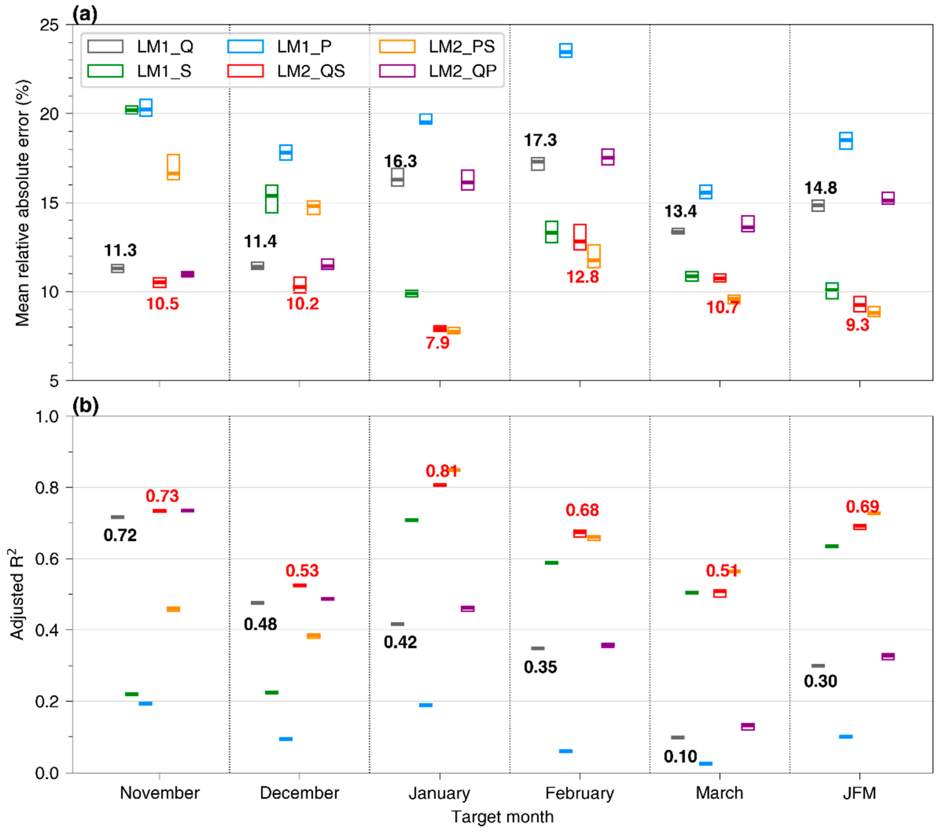
| Month | LM1_Q | LM2_QS | ||||
|---|---|---|---|---|---|---|
| Mean | Min | Max | Mean | Min | Max | |
| November | 17.31 | 17.07 | 19.25 | 19.11 | 18.83 | 21.07 |
| December | 19.24 | 18.71 | 23.82 | 20.57 | 20.03 | 25.17 |
| January | 18.71 | 18.40 | 21.50 | 15.95 | 15.76 | 17.30 |
| February | 19.69 | 19.37 | 23.00 | 17.73 | 17.47 | 19.79 |
| March | 22.81 | 22.19 | 28.36 | 19.76 | 19.27 | 23.43 |
| JFM | 20.21 | 19.79 | 24.19 | 17.40 | 17.10 | 19.80 |
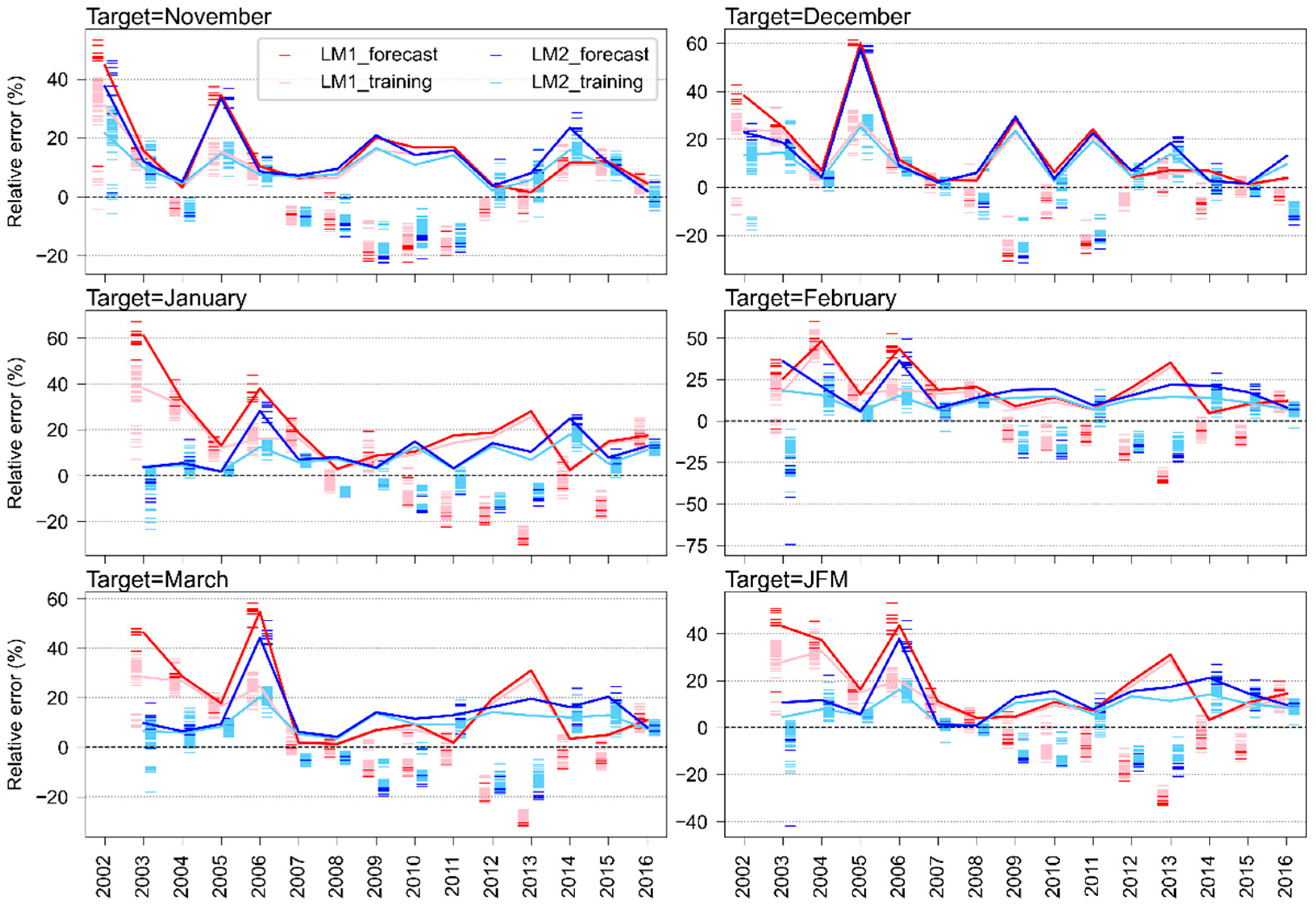
| Year | LM1_Q | LM2_QS | ||||||||||
|---|---|---|---|---|---|---|---|---|---|---|---|---|
| November | December | January | February | March | JFM | November | December | January | February | March | JFM | |
| 2002 | 34.3 | 26.1 | - | - | - | - | 24.5 | 14.0 | - | - | - | - |
| 2003 | 14.5 | 23.6 | 42.2 | 23.2 | 32.7 | 32.8 | 9.6 | 14.6 | −2.1 | −15.6 | 5.8 | −2.9 |
| 2004 | −2.9 | 6.5 | 30.7 | 44.8 | 26.3 | 32.9 | −4.7 | 3.7 | 3.8 | 14.0 | 4.7 | 6.7 |
| 2005 | 16.7 | 28.9 | 12.2 | 17.0 | 17.1 | 15.4 | 15.8 | 27.2 | 1.7 | 5.8 | 8.3 | 5.3 |
| 2006 | 9.4 | 11.2 | 17.7 | 20.1 | 25.1 | 21.3 | 7.6 | 8.5 | 13.4 | 16.1 | 20.7 | 17.0 |
| 2007 | −6.1 | 2.9 | 16.0 | 18.4 | 0.9 | 10.1 | −6.8 | 1.9 | 5.7 | 7.1 | −5.4 | 1.0 |
| 2008 | −6.7 | −2.3 | −2.5 | 19.0 | 0.2 | 4.0 | −8.2 | −5.1 | −7.3 | 12.2 | −3.9 | −0.7 |
| 2009 | −16.8 | −23.6 | 6.9 | −7.4 | −8.1 | −3.7 | −17.4 | −24.5 | −2.7 | −15.5 | −14.6 | −11.6 |
| 2010 | −14.5 | −4.1 | −9.5 | −12.8 | −7.7 | −10.0 | −11.0 | 2.0 | −13.4 | −16.3 | −11.0 | −13.5 |
| 2011 | −15.7 | −21.5 | −14.8 | −5.0 | −1.4 | −6.7 | −14.6 | −19.6 | −2.6 | 9.1 | 10.1 | 5.7 |
| 2012 | −3.9 | −4.1 | −17.4 | −18.3 | −18.9 | −18.2 | 1.5 | 5.0 | −13.1 | −13.4 | −15.1 | −14.0 |
| 2013 | 0.6 | 6.1 | −25.8 | −32.8 | −28.5 | −29.1 | 6.1 | 15.0 | −7.6 | −15.2 | −13.9 | −12.3 |
| 2014 | 10.9 | −6.3 | −1.0 | −3.3 | −2.5 | −2.3 | 16.6 | 1.7 | 18.9 | 17.0 | 13.1 | 16.0 |
| 2015 | 11.0 | 0.4 | −14.4 | −9.5 | −5.0 | −9.4 | 10.6 | −0.2 | 5.5 | 12.1 | 13.5 | 10.5 |
| 2016 | 4.3 | −3.0 | 16.0 | 12.8 | 10.3 | 12.9 | −0.5 | −10.0 | 11.1 | 7.3 | 7.4 | 8.4 |
| Month | LM1_Dry | LM2_Dry | Diff (%) | LM1_Wet | LM2_Wet | Diff (%) |
|---|---|---|---|---|---|---|
| November | 17.2 | 13.6 | 20.8 | 16.6 | 16.1 | 2.9 |
| December | 12.9 | 12.2 | 5.3 | 15.6 | 15.9 | −2.4 |
| January | 24.6 | 7.5 | 69.5 | 17.7 | 10.9 | 38.1 |
| February | 27.3 | 13.7 | 49.6 | 20.6 | 15.1 | 26.7 |
| March | 25.0 | 7.5 | 69.8 | 18.6 | 12.2 | 34.5 |
| JFM | 25.4 | 7.6 | 70.1 | 19.1 | 12.7 | 33.4 |
Publisher’s Note: MDPI stays neutral with regard to jurisdictional claims in published maps and institutional affiliations. |
© 2021 by the authors. Licensee MDPI, Basel, Switzerland. This article is an open access article distributed under the terms and conditions of the Creative Commons Attribution (CC BY) license (https://creativecommons.org/licenses/by/4.0/).
Share and Cite
Liu, X.; Tang, Q.; Hosseini-Moghari, S.-M.; Shi, X.; Lo, M.-H.; Scanlon, B. GRACE Satellites Enable Long-Lead Forecasts of Mountain Contributions to Streamflow in the Low-Flow Season. Remote Sens. 2021, 13, 1993. https://doi.org/10.3390/rs13101993
Liu X, Tang Q, Hosseini-Moghari S-M, Shi X, Lo M-H, Scanlon B. GRACE Satellites Enable Long-Lead Forecasts of Mountain Contributions to Streamflow in the Low-Flow Season. Remote Sensing. 2021; 13(10):1993. https://doi.org/10.3390/rs13101993
Chicago/Turabian StyleLiu, Xingcai, Qiuhong Tang, Seyed-Mohammad Hosseini-Moghari, Xiaogang Shi, Min-Hui Lo, and Bridget Scanlon. 2021. "GRACE Satellites Enable Long-Lead Forecasts of Mountain Contributions to Streamflow in the Low-Flow Season" Remote Sensing 13, no. 10: 1993. https://doi.org/10.3390/rs13101993
APA StyleLiu, X., Tang, Q., Hosseini-Moghari, S.-M., Shi, X., Lo, M.-H., & Scanlon, B. (2021). GRACE Satellites Enable Long-Lead Forecasts of Mountain Contributions to Streamflow in the Low-Flow Season. Remote Sensing, 13(10), 1993. https://doi.org/10.3390/rs13101993