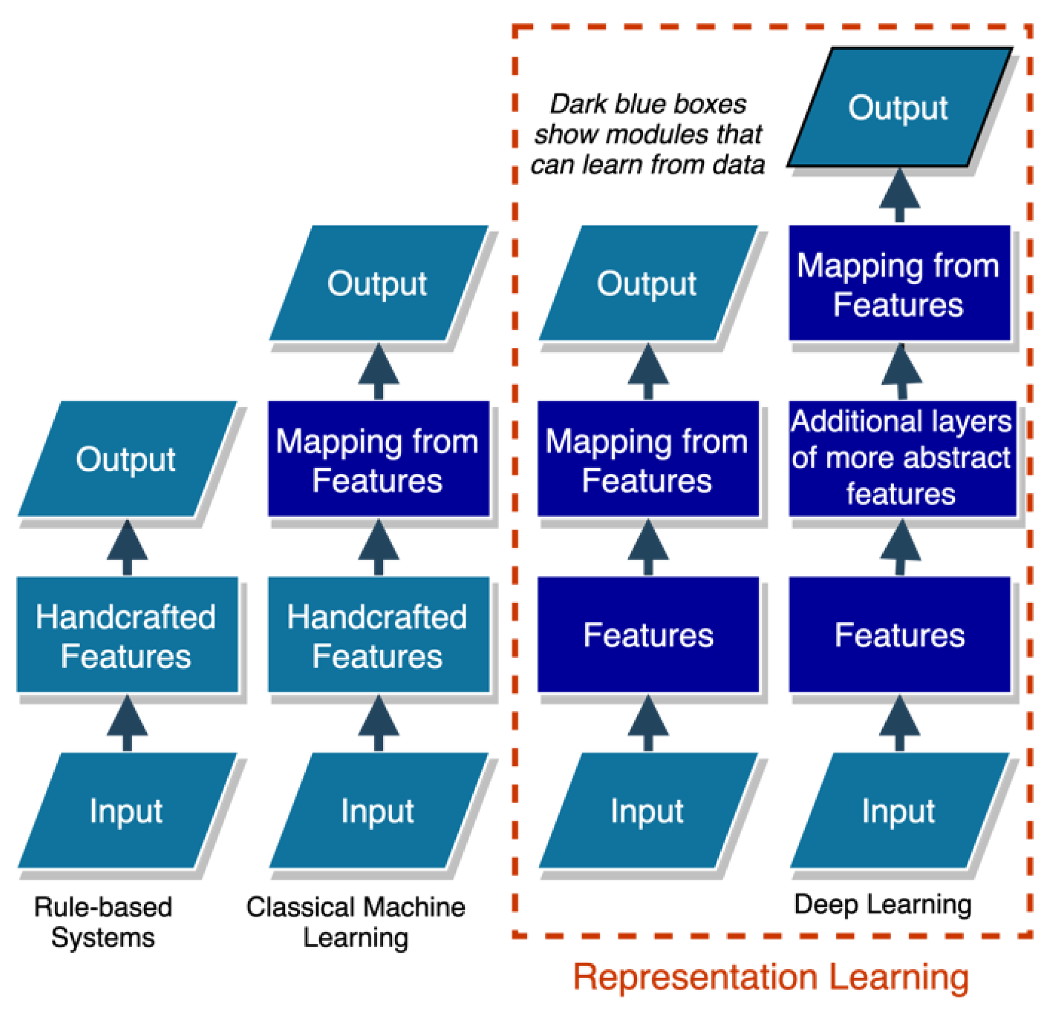
Figure 1.
AI approaches for data classification (adapted from Goodfellow et al. [
22]).
Figure 1.
AI approaches for data classification (adapted from Goodfellow et al. [
22]).
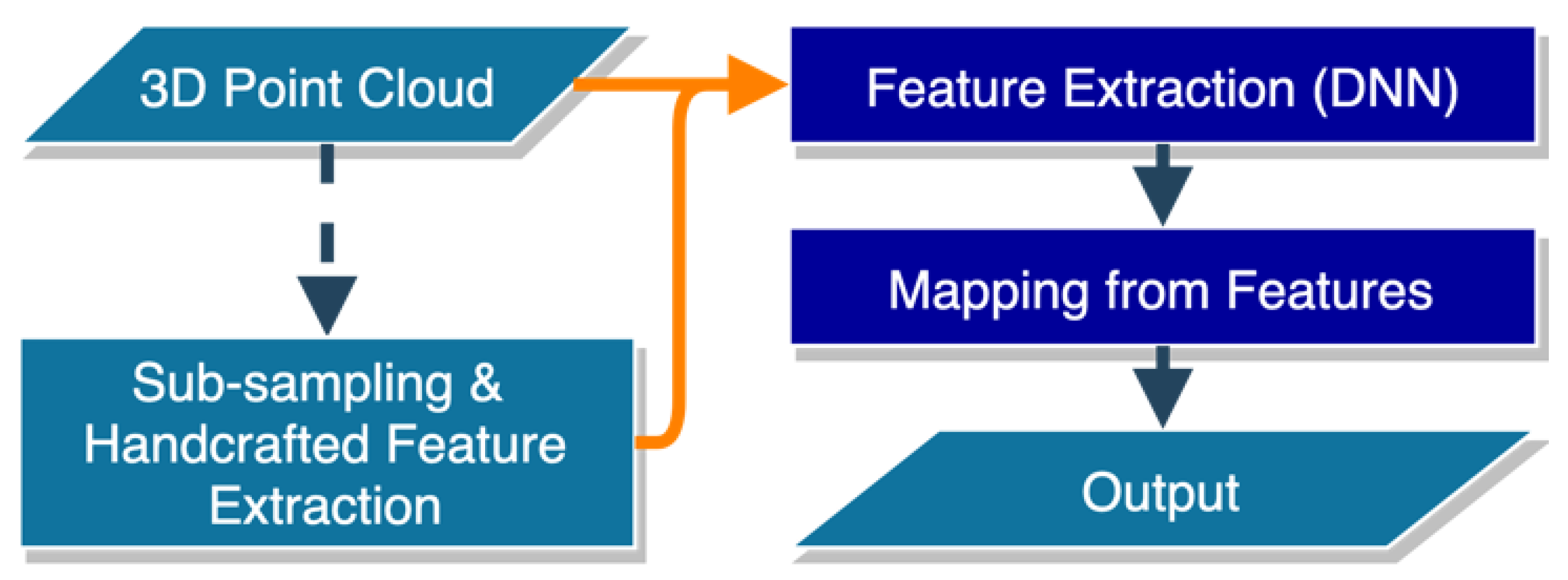
Figure 2.
The proposed classification framework based on deep learning (modules that can learn from the given data are shown with dark blue boxes).
Figure 2.
The proposed classification framework based on deep learning (modules that can learn from the given data are shown with dark blue boxes).
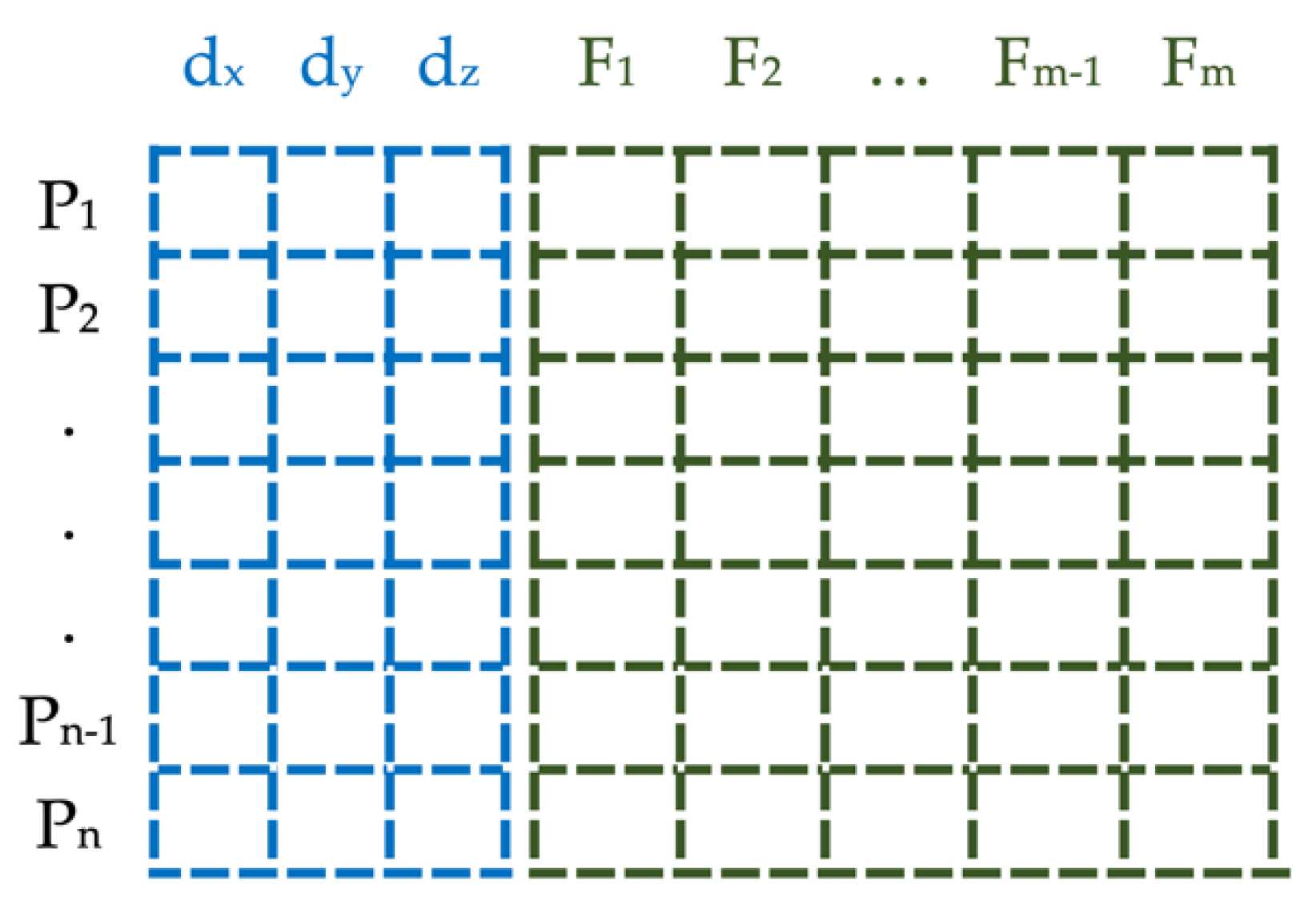
Figure 3.
2D patches generated for each 3D point of the cloud: Pn denotes points, dx,y,z denotes patch-wise scaled coordinates (blue cells) and Fm denotes the available/computed features (green cells).
Figure 3.
2D patches generated for each 3D point of the cloud: Pn denotes points, dx,y,z denotes patch-wise scaled coordinates (blue cells) and Fm denotes the available/computed features (green cells).
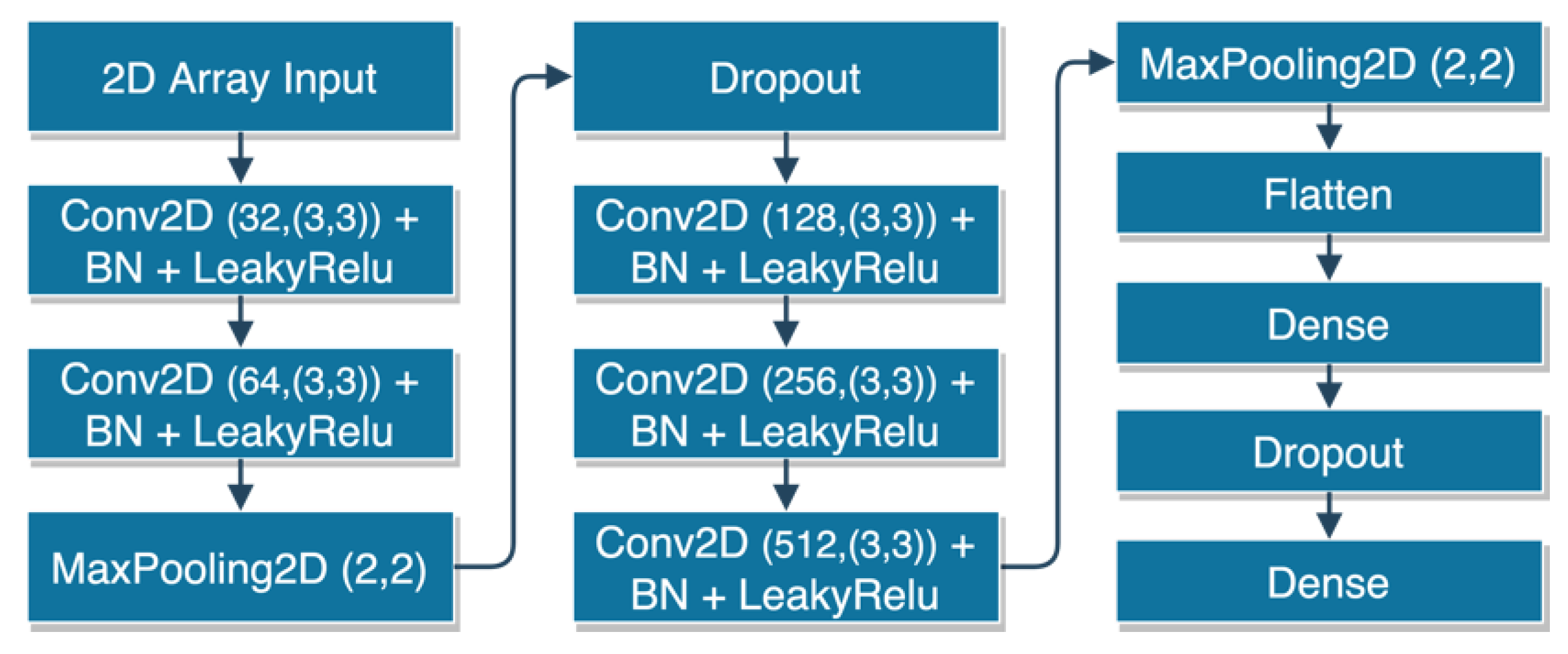
Figure 4.
Our 2DCNN structure (BN stands for batch normalization layer).
Figure 4.
Our 2DCNN structure (BN stands for batch normalization layer).
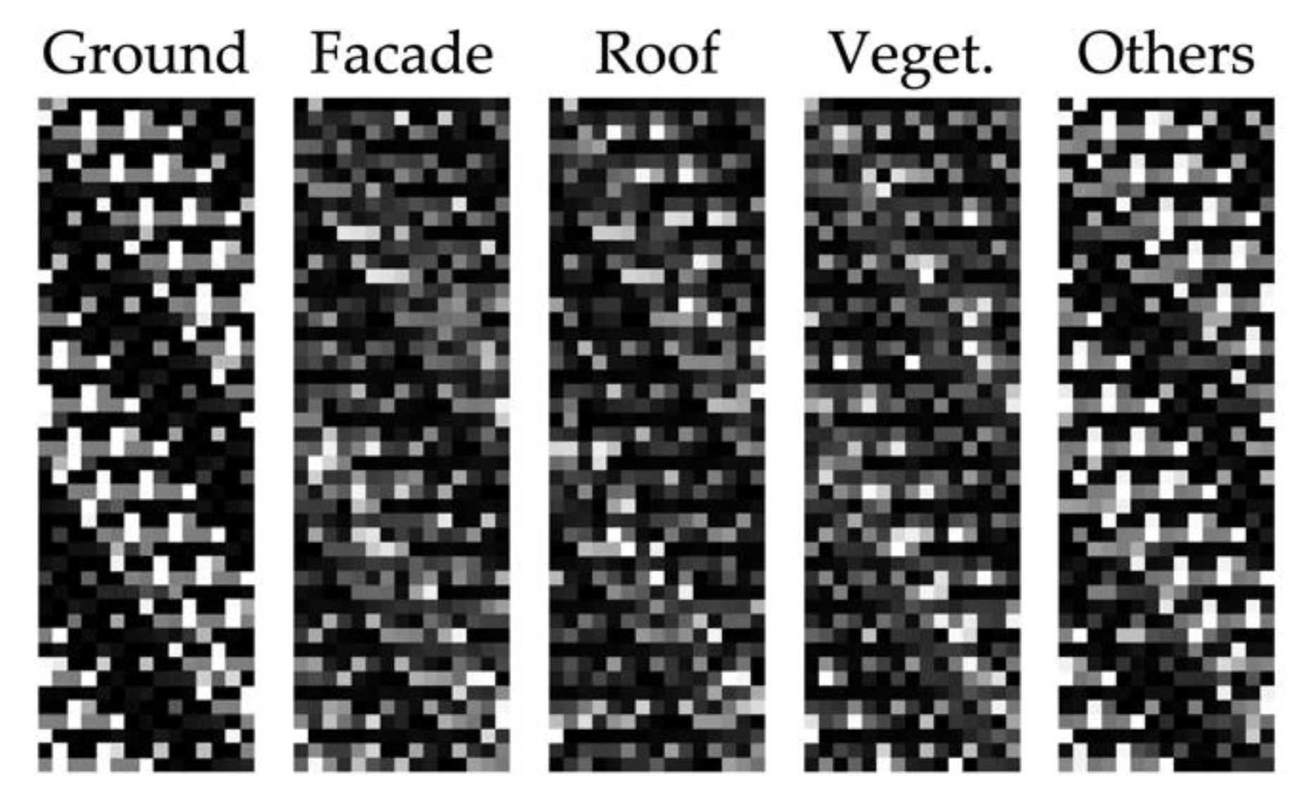
Figure 5.
An example of 2D patch visualization (transposed for better picturing).
Figure 5.
An example of 2D patch visualization (transposed for better picturing).
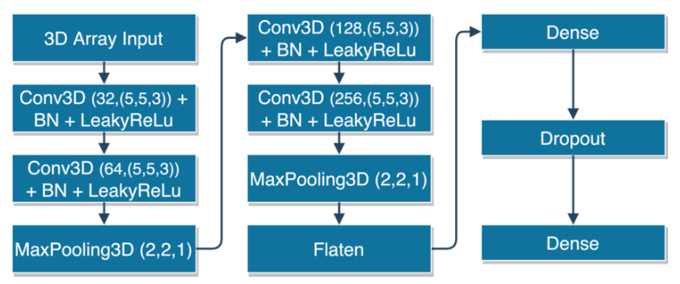
Figure 6.
Our 3DCNN structure.
Figure 6.
Our 3DCNN structure.
Figure 7.
An example of generated 3D patches (transposed for better pitcuring).
Figure 7.
An example of generated 3D patches (transposed for better pitcuring).
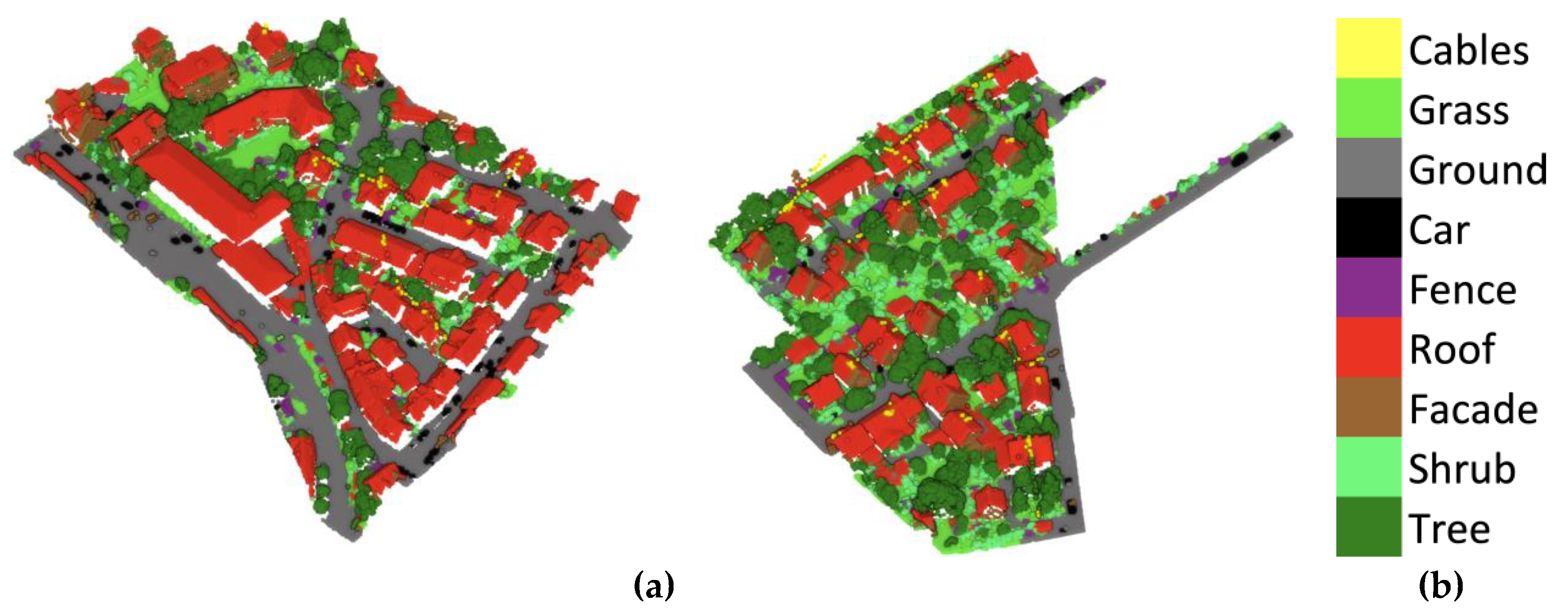
Figure 8.
ISPRS Vaihingen point cloud with its nine classes. (a) Training, (b) test sections and (c) legend.
Figure 8.
ISPRS Vaihingen point cloud with its nine classes. (a) Training, (b) test sections and (c) legend.
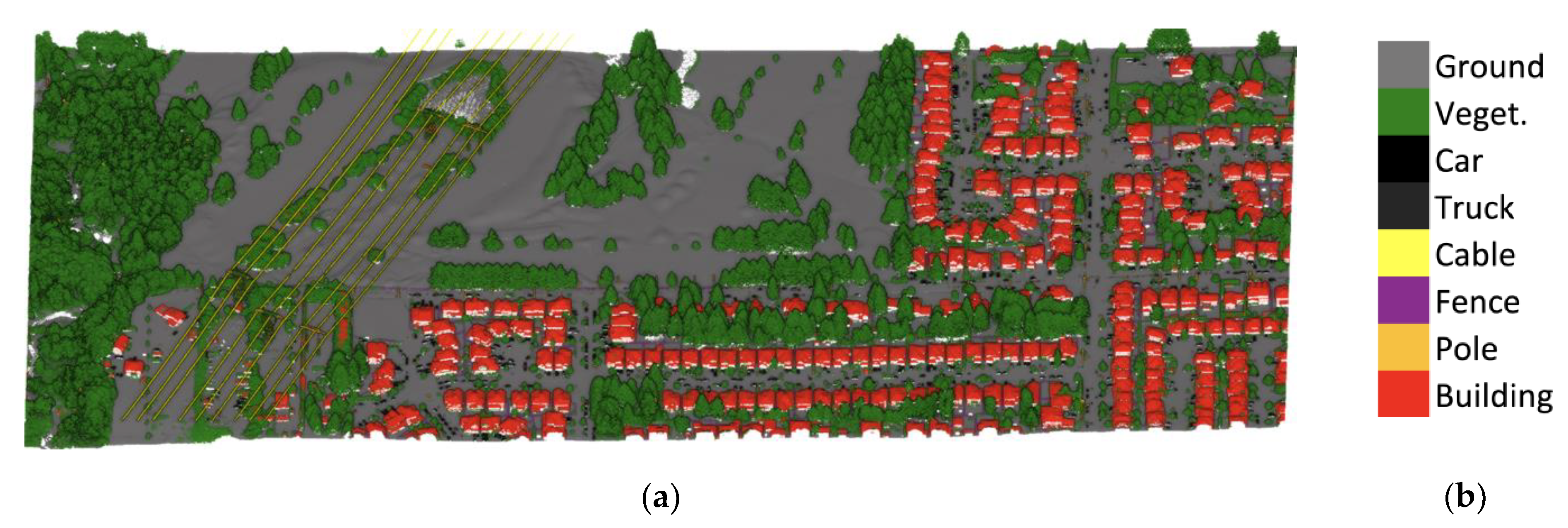
Figure 9.
(a) DALES point cloud with its eight classes (b) legend.
Figure 9.
(a) DALES point cloud with its eight classes (b) legend.
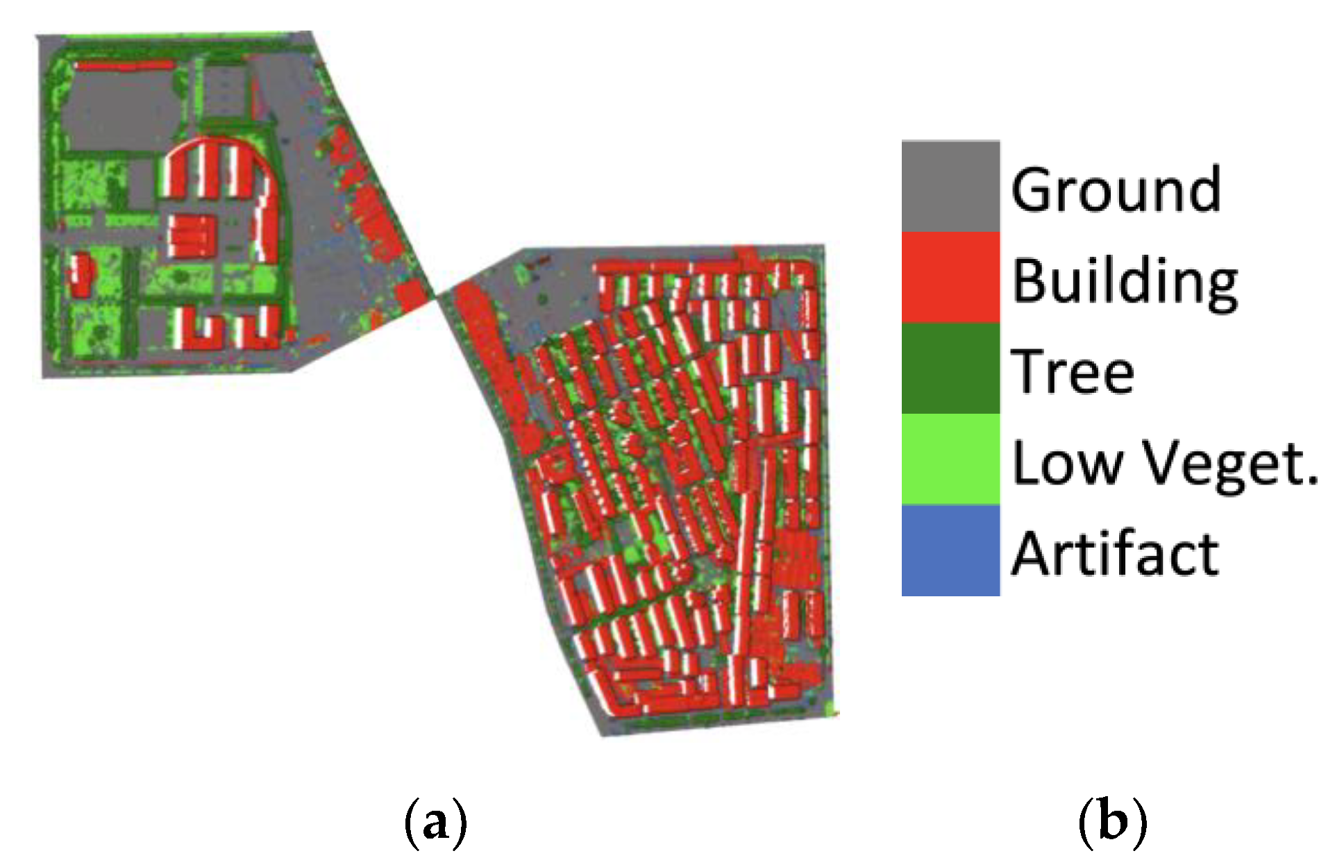
Figure 10.
LASDU point cloud with its five classes (a). Training (red) and test (blue) sections (b). (c) Legend.
Figure 10.
LASDU point cloud with its five classes (a). Training (red) and test (blue) sections (b). (c) Legend.
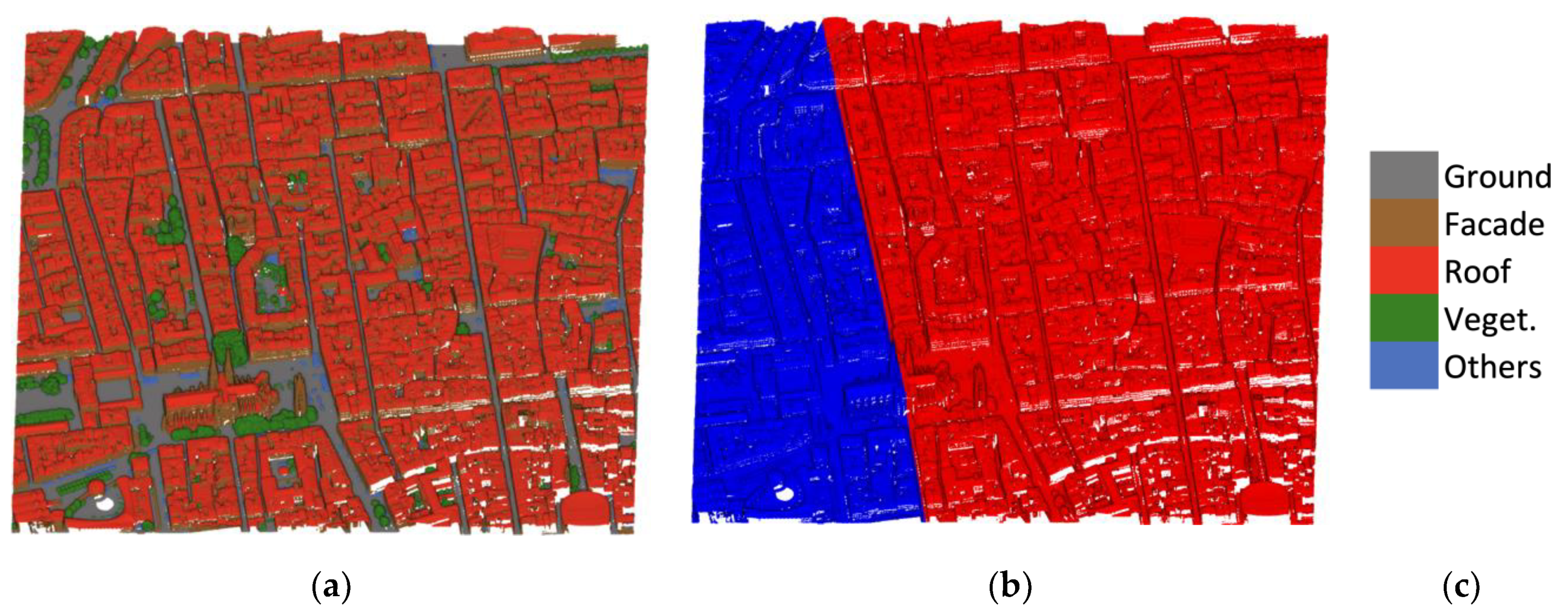
Figure 11.
Bordeaux point cloud with its five classes (a). The dataset is separated (b) into training (~70%, blue) and test (~30%, red). (c) Legend.
Figure 11.
Bordeaux point cloud with its five classes (a). The dataset is separated (b) into training (~70%, blue) and test (~30%, red). (c) Legend.
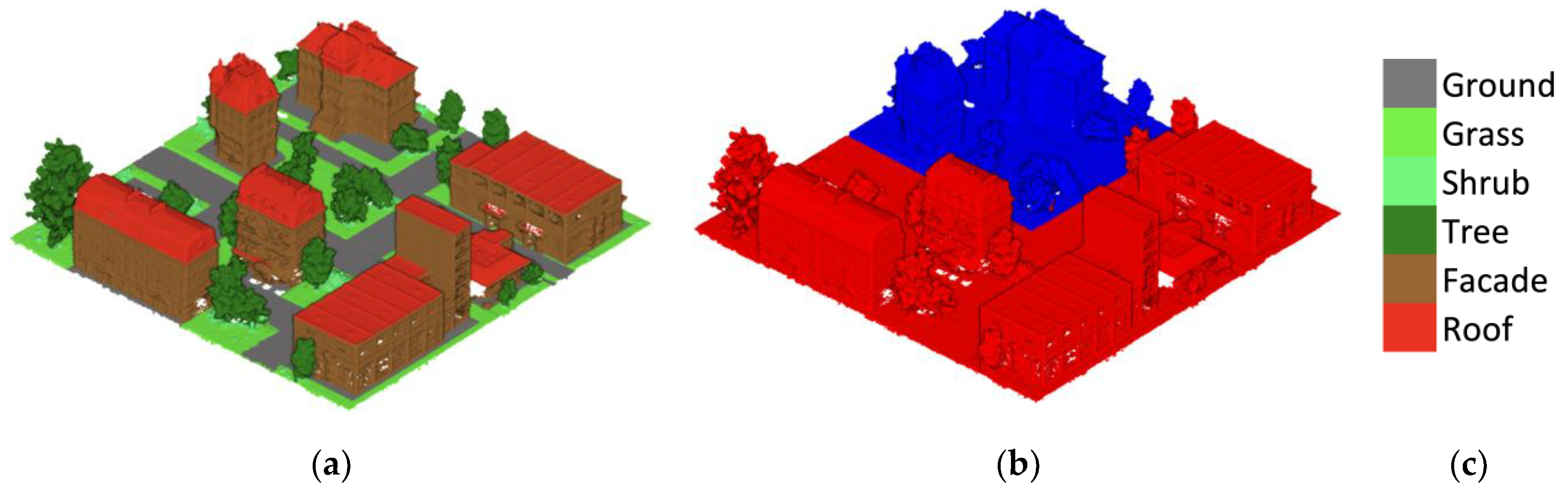
Figure 12.
3DOMCity point cloud and its six classes (a). The dataset is separated (b) into training (~70%, blue) and test (~30%, red). (c) Legend.
Figure 12.
3DOMCity point cloud and its six classes (a). The dataset is separated (b) into training (~70%, blue) and test (~30%, red). (c) Legend.
Figure 13.
(a) Classification result of the ISPRS Vaihingen dataset with the 2DCNN approach. (b). Legend.
Figure 13.
(a) Classification result of the ISPRS Vaihingen dataset with the 2DCNN approach. (b). Legend.
Figure 14.
(a) Classification result of both DALES tiles with our 3DCNN, (b) legend.
Figure 14.
(a) Classification result of both DALES tiles with our 3DCNN, (b) legend.
Figure 15.
(a) 3DCNN classification results on the testing area of the LASDU dataset, (b) legend.
Figure 15.
(a) 3DCNN classification results on the testing area of the LASDU dataset, (b) legend.
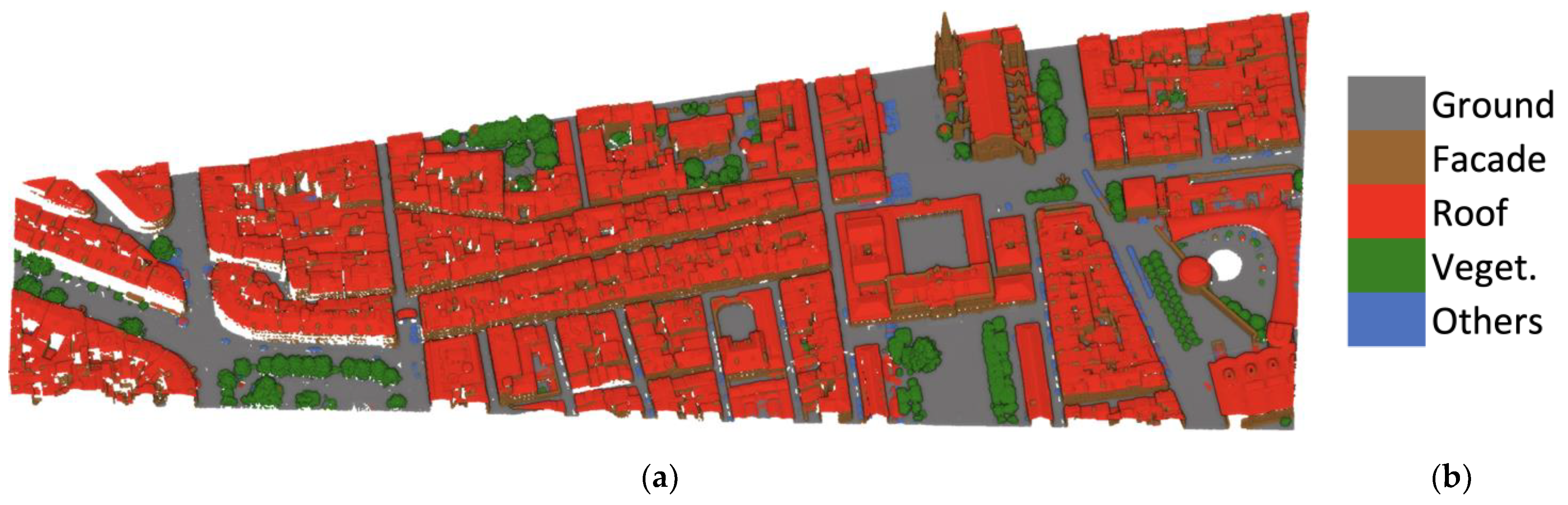
Figure 16.
(a) Classification result on the testing area of the Bordeaux dataset with our 2DCNN, (b) legend.
Figure 16.
(a) Classification result on the testing area of the Bordeaux dataset with our 2DCNN, (b) legend.
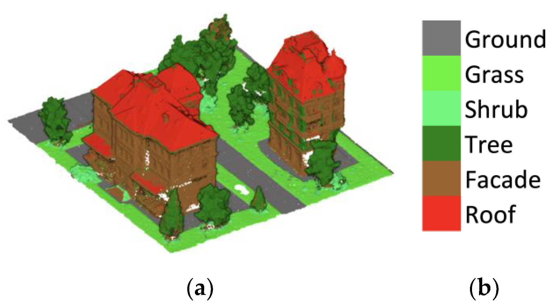
Figure 17.
(a) Classification result on testing area of the 3DOMCity dataset with our 2DCNN, (b) legend.
Figure 17.
(a) Classification result on testing area of the 3DOMCity dataset with our 2DCNN, (b) legend.
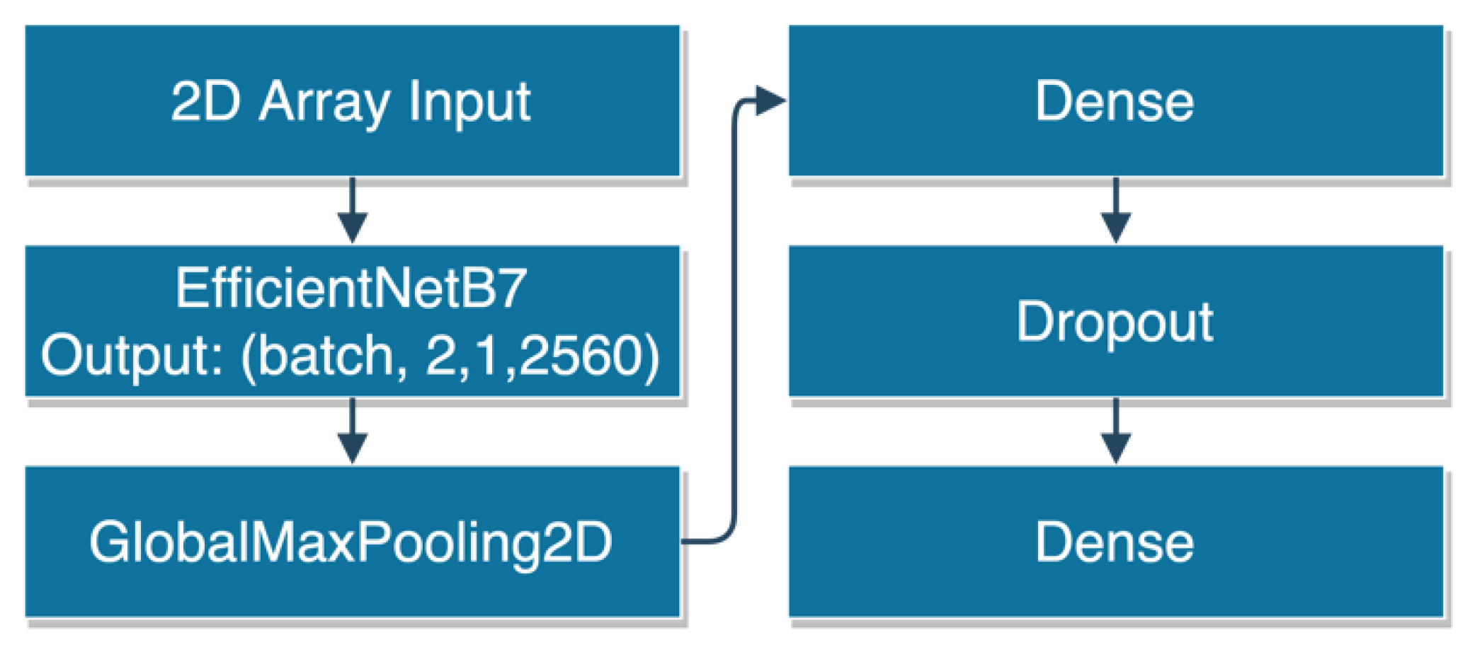
Figure 18.
Implementation of EfficientNetb7 from TensorFlow library.
Figure 18.
Implementation of EfficientNetb7 from TensorFlow library.
Table 1.
Employed handcrafted features.
Table 1.
Employed handcrafted features.
| Linearity | |
| Sphericity | |
| Omnivariance | |
| Local Elevation Change | |
| Local Planarity | |
| Vertical Angle | |
| Height Above Ground | |
Table 2.
Summary of the used datasets (L: LiDAR, OP: Oblique Photogrammetry, lab: laboratory).
Table 2.
Summary of the used datasets (L: LiDAR, OP: Oblique Photogrammetry, lab: laboratory).
| Dataset (Year) | Source | Points | Density (pts/m2) | Resolution (m) | Coverage
(m × m) (Tiles) | RGB | Classes |
|---|
| ISPRS Vaihingen (2013) [51] | L | 1,165,598 | 4 | 0.258 | Train: 383 × 405
Test: 374 × 402 | NIR | 9 |
DALES
(2020) [52] | L | 497,632,442 | 35 | 0.116 | 500 × 500 (40 tiles) | No | 8 |
LASDU
(2020) [53,54] | L | 3,080,856 | 3 | 0.484 | 1071 × 1285 | No | 5 |
Bordeaux
(2020) [55] | L + OP | 10,230,941 | 25 | 0.173 | 704 × 739 | Yes | 5 |
3DOMCity
(2019) [56] | OP (lab.) | 22,825,024 | 14000 | 0.158mm | 0.813 × 0.811 | Yes | 6 |
Table 3.
Density analysis on the ISPRS Vaihingen dataset.
Table 3.
Density analysis on the ISPRS Vaihingen dataset.
| Leaf Coeff. | % of Points | Resol. (m) | Min. knn | Mean knn | Median knn | Max. knn | Std. knn | Weigh. F1 | OA |
|---|
| 1 | 100 | 0.258 | 2 | 11 | 5 | 106 | 12.99 | 0.788 | 0.788 |
| 2 | 50 | 0.434 | 2 | 4 | 5 | 15 | 1.51 | 0.798 | 0.796 |
| 4 | 20 | 0.732 | 2 | 4 | 4 | 13 | 1.31 | 0.776 | 0.788 |
| 6 | 11 | 1.07 | 2 | 4 | 3 | 13 | 1.37 | 0.768 | 0.770 |
Table 4.
Density analysis on LASDU dataset.
Table 4.
Density analysis on LASDU dataset.
| Leaf Coeff. | % of Points | Resol. (m) | Min. knn | Mean knn | Median knn | Max. knn | Std. knn | Weigh. F1 | OA |
|---|
| 1 | 100 | 0.484 | 2 | 4 | 4 | 83 | 1.45 | 0.826 | 0.814 |
| 2 | 48 | 0.792 | 2 | 5 | 4 | 12 | 1.24 | 0.823 | 0.821 |
| 4 | 15 | 1.440 | 2 | 5 | 5 | 14 | 1.31 | 0.805 | 0.816 |
Table 5.
Density Analysis on Bordeaux dataset.
Table 5.
Density Analysis on Bordeaux dataset.
| Leaf Coeff. | % of Points | Resol. (m) | Min. knn | Mean knn | Median knn | Max. knn | Std. knn | Weigh. F1 | OA |
|---|
| 1 | 100 | 0.173 | 2 | 6 | 2 | 61 | 6.01 | 0.930 | 0.928 |
| 4 | 23 | 0.528 | 2 | 4 | 2 | 14 | 1.44 | 0.922 | 0.942 |
| 6 | 12 | 0.737 | 2 | 4 | 4 | 12 | 1.31 | 0.940 | 0.940 |
| 8 | 8 | 0.946 | 2 | 4 | 4 | 12 | 1.32 | 0.935 | 0.935 |
Table 6.
Number of points in each dataset before and after the downsampling procedure.
Table 6.
Number of points in each dataset before and after the downsampling procedure.
| Dataset | ISPRS Vaihingen | DALES | LASDU | Bordeaux | 3DOMCity |
|---|
| # of original points | 1,165,598 | 497,632,442 | 3,080,856 | 10,230,941 | 22,825,024 |
| # of downsampled points | 236,603 | 27,652,837 | 1,465,068 | 1,264,690 | 2,075,937 |
| % of kept points | 0.203 | 0.056 | 0.476 | 0.124 | 0.091 |
Table 7.
Average and weighted F1 and IoU scores for 2DCNN and 3DCNN classifiers on the ISPRS Vaihingen dataset (LV: low vegetation). The OA is also reported.
Table 7.
Average and weighted F1 and IoU scores for 2DCNN and 3DCNN classifiers on the ISPRS Vaihingen dataset (LV: low vegetation). The OA is also reported.
| | Cables | LV | Ground | Car | Fence | Roof | Facade | Shrub | Tree | Average | Weighted | OA |
|---|
| 2DCNN-F1 | 0.000 | 0.795 | 0.904 | 0.733 | 0.213 | 0.929 | 0.583 | 0.451 | 0.817 | 0.603 | 0.822 | 0.826 |
| 3DCNN-F1 | 0.301 | 0.781 | 0.896 | 0.688 | 0.207 | 0.902 | 0.536 | 0.413 | 0.802 | 0.614 | 0.804 | 0.806 |
| 2DCNN-IoU | 0.000 | 0.660 | 0.825 | 0.579 | 0.119 | 0.867 | 0.411 | 0.291 | 0.690 | 0.494 | 0.719 | 0.826 |
| 3DCNN-IoU | 0.177 | 0.641 | 0.811 | 0.525 | 0.116 | 0.822 | 0.367 | 0.261 | 0.670 | 0.488 | 0.693 | 0.806 |
Table 8.
Average and weighted F1 and IoU scores for 2DCNN and 3DCNN classifiers on the DALES dataset. The OA is also reported.
Table 8.
Average and weighted F1 and IoU scores for 2DCNN and 3DCNN classifiers on the DALES dataset. The OA is also reported.
| | Ground | Veget. | Car | Truck | Cable | Fence | Pole | Building | Avg. | Weighted | OA |
|---|
| 2DCNN-F1 | 0.962 | 0.927 | 0.666 | 0.000 | 0.903 | 0.530 | 0.468 | 0.911 | 0.671 | 0.937 | 0.938 |
| 3DCNN-F1 | 0.958 | 0.923 | 0.682 | 0.000 | 0.914 | 0.490 | 0.547 | 0.905 | 0.677 | 0.932 | 0.934 |
| 2DCNN-IoU | 0.926 | 0.863 | 0.499 | 0.000 | 0.823 | 0.360 | 0.306 | 0.837 | 0.577 | 0.884 | 0.938 |
| 3DCNN-IoU | 0.919 | 0.857 | 0.517 | 0.000 | 0.841 | 0.325 | 0.377 | 0.826 | 0.583 | 0.876 | 0.934 |
Table 9.
Average and weighted F1 and IoU scores for 2DCNN and 3DCNN classifiers for the LASDU dataset. The OA is also reported.
Table 9.
Average and weighted F1 and IoU scores for 2DCNN and 3DCNN classifiers for the LASDU dataset. The OA is also reported.
| | Ground | Building | Tree | LV | Artifact | Average | Weighted | OA |
|---|
| 2DCNN-F1 | 0.887 | 0.935 | 0.860 | 0.691 | 0.360 | 0.746 | 0.851 | 0.846 |
| 3DCNN-F1 | 0.885 | 0.915 | 0.858 | 0.673 | 0.322 | 0.730 | 0.840 | 0.837 |
| 2DCNN-IoU | 0.796 | 0.878 | 0.754 | 0.527 | 0.220 | 0.635 | 0.757 | 0.846 |
| 3DCNN-IoU | 0.793 | 0.843 | 0.751 | 0.507 | 0.192 | 0.617 | 0.741 | 0.837 |
Table 10.
Average and weighted F1 and IoU scores for 2DCNN and 3DCNN classifiers for the Bordeaux dataset. The OA is also reported.
Table 10.
Average and weighted F1 and IoU scores for 2DCNN and 3DCNN classifiers for the Bordeaux dataset. The OA is also reported.
| | Ground | Facade | Roof | Vegetation | Others | Average | Weighted | OA |
|---|
| 2DCNN-F1 | 0.972 | 0.819 | 0.956 | 0.986 | 0.708 | 0.888 | 0.943 | 0.944 |
| 3DCNN-F1 | 0.966 | 0.807 | 0.951 | 0.985 | 0.682 | 0.878 | 0.937 | 0.938 |
| 2DCNN-IoU | 0.945 | 0.694 | 0.916 | 0.972 | 0.548 | 0.808 | 0.897 | 0.944 |
| 3DCNN-IoU | 0.934 | 0.676 | 0.907 | 0.970 | 0.517 | 0.801 | 0.887 | 0.938 |
Table 11.
Average and weighted F1 and IoU scores for 2DCNN and 3DCNN classifiers for the 3DOMCity dataset. The OA is also reported.
Table 11.
Average and weighted F1 and IoU scores for 2DCNN and 3DCNN classifiers for the 3DOMCity dataset. The OA is also reported.
| | Ground | Grass | Shrub | Tree | Facade | Roof | Average | Weighted | OA |
|---|
| 2DCNN-F1 | 0.945 | 0.936 | 0.798 | 0.878 | 0.864 | 0.906 | 0.888 | 0.889 | 0.889 |
| 3DCNN-F1 | 0.954 | 0.938 | 0.777 | 0.864 | 0.866 | 0.887 | 0.881 | 0.883 | 0.883 |
| 2DCNN-IoU | 0.897 | 0.880 | 0.664 | 0.782 | 0.761 | 0.828 | 0.802 | 0.802 | 0.889 |
| 3DCNN-IoU | 0.913 | 0.883 | 0.635 | 0.760 | 0.763 | 0.796 | 0.792 | 0.793 | 0.883 |
Table 12.
Performance comparison between our methods and recent papers, ordered by OA. (* difference from the highest OA score in the table).
Table 12.
Performance comparison between our methods and recent papers, ordered by OA. (* difference from the highest OA score in the table).
| Method | GPU TFLOPS FP32 | Training Time (Hours) | GPU Watt | GPU Memory | OA | GPU |
|---|
| Li et al. [37] | 8.73 | 10 | 250 | 24 GB | 0.839 | Nvidia Tesla K80 |
| Li et al. [21] | 2 × 12.15 | 7 | 2 × 250 | 2 × 12 GB | 0.835 | 2 × Nvidia Titan Xp |
| Wen et al. [35] | 12.15 | 10 | 250 | 12 GB | 0.832 | Nvidia Titan Xp |
| Chen et al. [39] | 14.13 | 2 | 250 | 32 GB | 0.832 | Nvidia Tesla V100 |
| EfficientNetB7 [57] | 13.45 | 1 | 250 | 11 GB | 0.748 (−9.1% *) | Nvidia RTX 2080Ti |
| Ours (2DCNN) | 13.45 | 0.15 | 250 | 11 GB | 0.826 (−1.3% *) | Nvidia RTX 2080Ti |
| Ours (3DCNN) | 13.45 | 0.5 | 250 | 11 GB | 0.806 (−3.3% *) | Nvidia RTX 2080Ti |
Table 13.
OA scores for 2DCNN and 3DCNN classifiers for DALES dataset.
Table 13.
OA scores for 2DCNN and 3DCNN classifiers for DALES dataset.
| | Ground | Vegetation | Car | Truck | Cable | Fence | Pole | Building | OA |
|---|
| KPConv [40] | 0.971 | 0.941 | 0.853 | 0.419 | 0.955 | 0.635 | 0.750 | 0.966 | 0.978 |
| PointNet++ [32] | 0.941 | 0.912 | 0.754 | 0.303 | 0.799 | 0.462 | 0.400 | 0.891 | 0.957 |
| Ours (2DCNN) | 0.926 | 0.863 | 0.499 | 0.000 | 0.823 | 0.360 | 0.306 | 0.837 | 0.938 |
| Ours (3DCNN) | 0.919 | 0.857 | 0.517 | 0.000 | 0.841 | 0.325 | 0.377 | 0.826 | 0.934 |
Table 14.
Comparison of F1 scores and OA on the LASDU dataset with respect to current state-of-the-art methods.
Table 14.
Comparison of F1 scores and OA on the LASDU dataset with respect to current state-of-the-art methods.
| | Ground | Building | Tree | LV | Artifact | Avg. F1 | OA |
|---|
| Ours (2DCNN) | 0.887 | 0.935 | 0.860 | 0.691 | 0.360 | 0.746 | 0.846 |
| Ours (3DCNN) | 0.885 | 0.915 | 0.858 | 0.673 | 0.322 | 0.730 | 0.837 |
| PointNet++ [32] | 0.877 | 0.906 | 0.820 | 0.632 | 0.313 | 0.710 | 0.828 |
| HDA-PointNet++ [36] | 0.887 | 0.932 | 0.822 | 0.652 | 0.369 | 0.733 | 0.844 |
Table 15.
Averaged and weighted F1 and IoU scores for 2DCNN and 3DCNN classifiers trained on DALES dataset and predicting on ISPRS Vaihingen dataset. The OA is also reported.
Table 15.
Averaged and weighted F1 and IoU scores for 2DCNN and 3DCNN classifiers trained on DALES dataset and predicting on ISPRS Vaihingen dataset. The OA is also reported.
| | Cable | Ground | Car | Fence | Building | Vegetation | Average | Weighted | OA |
|---|
| 2DCNN DALES F1 | 0.130 | 0.926 | 0.399 | 0.001 | 0.759 | 0.397 | 0.435 | 0.753 | 0.779 |
| 3DCNN DALES F1 | 0.230 | 0.929 | 0.347 | 0.000 | 0.758 | 0.318 | 0.430 | 0.739 | 0.774 |
| 2DCNN DALES IoU | 0.069 | 0.862 | 0.249 | 0.000 | 0.611 | 0.247 | 0.340 | 0.649 | 0.779 |
| 3DCNN DALES IoU | 0.130 | 0.867 | 0.210 | 0.000 | 0.610 | 0.189 | 0.334 | 0.639 | 0.774 |
Table 16.
Corresponding classes between ISPRS Vaihingen and DALES datasets along with their distributions.
Table 16.
Corresponding classes between ISPRS Vaihingen and DALES datasets along with their distributions.
| ISPRS Vaihingen | Points (Test) | DALES | Points (Train) |
|---|
| Powerline | 0.2% | Cable | 29.7% |
| Low veget./Imp. Surface | 38.9% | Ground | 50.0% |
| Car | 0.8% | Car/Truck | 1.2% |
| Fence | 1.9% | Fence | 0.6% |
| Roof/Facade | 22.7% | Building/Pole | 0.9% |
| Shrub/Tree | 35.5% | Vegetation | 17.6% |
Table 17.
Average and weighted F1 and IoU scores for the 2DCNN and 3DCNN classifiers trained on DALES dataset and predicted on Bordeaux dataset. The OA is also reported.
Table 17.
Average and weighted F1 and IoU scores for the 2DCNN and 3DCNN classifiers trained on DALES dataset and predicted on Bordeaux dataset. The OA is also reported.
| | Ground | Building | Vegetation | Others | Average | Weighted | OA |
|---|
| 2DCNN DALES F1 | 0.965 | 0.978 | 0.947 | 0.434 | 0.831 | 0.968 | 0.969 |
| 3DCNN DALES F1 | 0.956 | 0.972 | 0.937 | 0.462 | 0.832 | 0.961 | 0.961 |
| 2DCNN DALES IoU | 0.931 | 0.958 | 0.900 | 0.277 | 0.766 | 0.941 | 0.969 |
| 3DCNN DALES IoU | 0.916 | 0.945 | 0.882 | 0.300 | 0.761 | 0.927 | 0.961 |
Table 18.
Corresponding classes between Bordeaux and DALES datasets.
Table 18.
Corresponding classes between Bordeaux and DALES datasets.
| Bordeaux | Points (Test) | DALES | Points (Train) |
|---|
| Ground | 13.9% | Ground | 29.7% |
| Roof/Facade | 80.2% | Building/Cable/Pole | 50.0% |
| Vegetation | 5.0% | Vegetation | 2.1% |
| Others | 1.0% | Car/Truck/Fence | 18.2% |
Table 19.
F1, IoU with 2DCNN and 3DCNN classifiers trained on ISPRS Vaihingen dataset and predicted on Bordeaux dataset. The OA is also reported.
Table 19.
F1, IoU with 2DCNN and 3DCNN classifiers trained on ISPRS Vaihingen dataset and predicted on Bordeaux dataset. The OA is also reported.
| | Ground | Facade | Roof | Vegetation | Others | Average | Weighted | OA |
|---|
| 2DCNN ISPRS F1 | 0.921 | 0.690 | 0.923 | 0.759 | 0.400 | 0.739 | 0.878 | 0.882 |
| 3DCNN ISPRS F1 | 0.882 | 0.743 | 0.878 | 0.832 | 0.331 | 0.733 | 0.855 | 0.855 |
| 2DCNN ISPRS IoU | 0.854 | 0.527 | 0.857 | 0.612 | 0.250 | 0.620 | 0.793 | 0.882 |
| 3DCNN ISPRS IoU | 0.789 | 0.591 | 0.782 | 0.712 | 0.198 | 0.614 | 0.751 | 0.855 |
Table 20.
Corresponding classes between Bordeaux and ISPRS Vaihingen datasets.
Table 20.
Corresponding classes between Bordeaux and ISPRS Vaihingen datasets.
| Bordeaux | Points (Test) | ISPRS Vaihingen | Points (Train) |
|---|
| Ground | 13.9% | Ground | 18.1% |
| Roof | 43.6% | Roof | 26.9% |
| Facade | 36.6% | facade | 5.1% |
| Vegetation | 5.0% | Low Veget./Shrub/Tree | 46.1% |
| Others | 1.0% | Cables/Car/Fence | 3.7% |
Table 21.
Summarized OA achieved in the different datasets considered in the evaluation procedures.
Table 21.
Summarized OA achieved in the different datasets considered in the evaluation procedures.
| | ISPRS Vaihingen | DALES | LASDU | Bordeaux | 3DOMCity |
|---|
| 2DCNN | 0.826 | 0.938 | 0.846 | 0.944 | 0.889 |
| 3DCNN | 0.806 | 0.934 | 0.837 | 0.938 | 0.883 |
Table 22.
Summarized OA for the generalization tests.
Table 22.
Summarized OA for the generalization tests.
| Trained on | Predicted on | Model | OA |
|---|
| DALES | ISPRS Vaihingen | 2DCNN | 0.779 |
| DALES | ISPRS Vaihingen | 3DCNN | 0.774 |
| DALES | Bordeaux | 2DCNN | 0.969 |
| DALES | Bordeaux | 3DCNN | 0.961 |
| ISPRS Vaihingen | Bordeaux | 2DCNN | 0.882 |
| ISPRS Vaihingen | Bordeaux | 3DCNN | 0.855 |


