
Maneuvering Target Detection Based on Subspace Subaperture Joint Coherent Integration


Abstract

1. Introduction
2. Mathematical Model
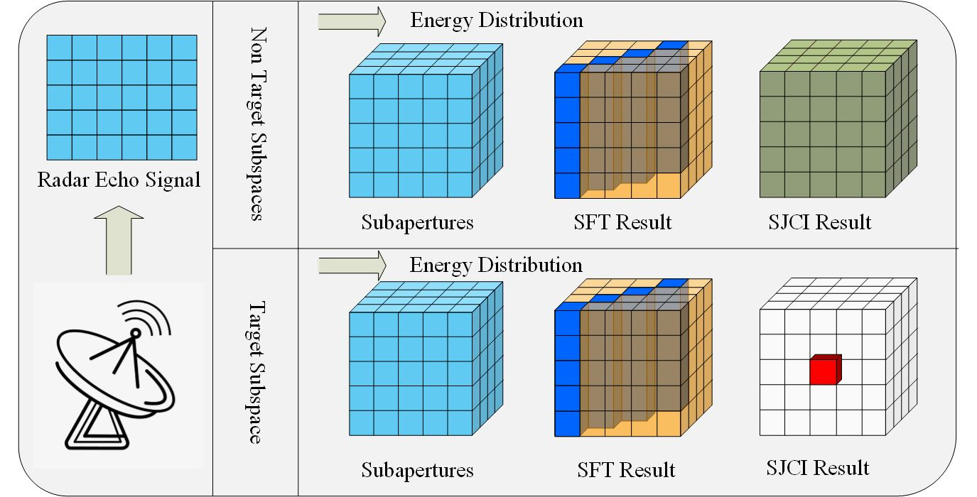
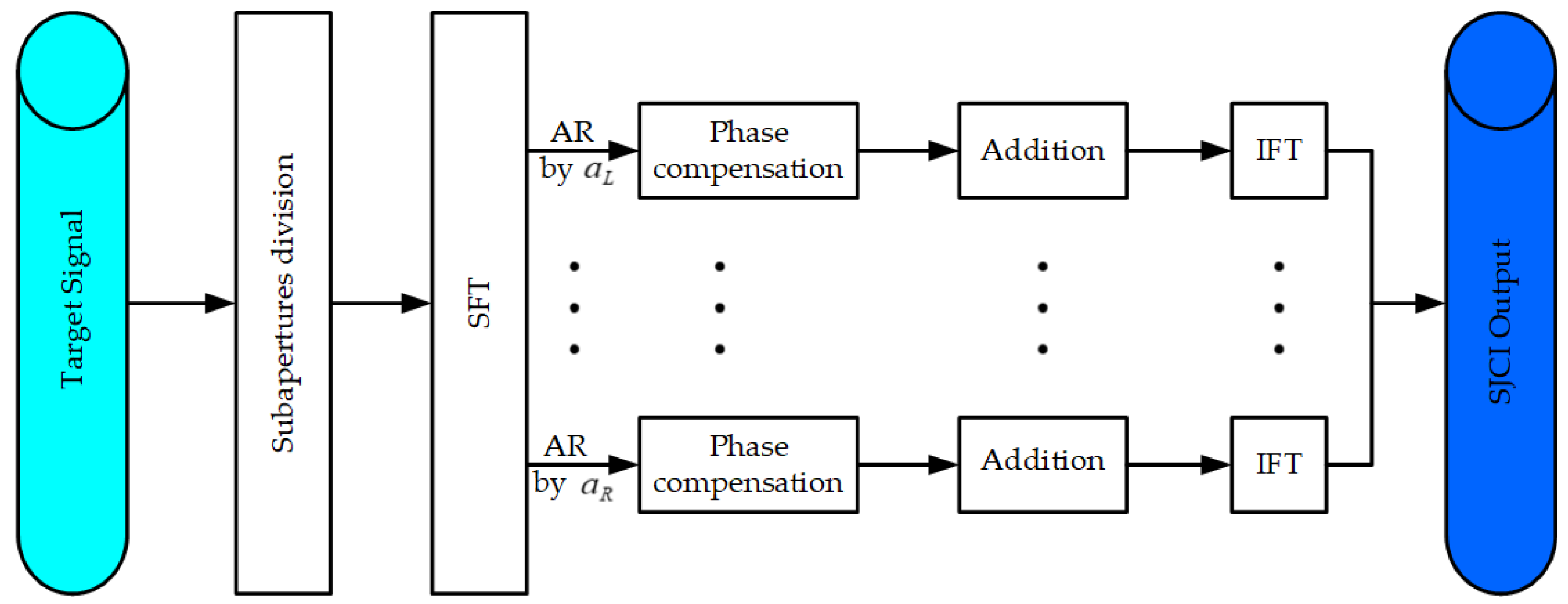
3. SJCI Algorithm
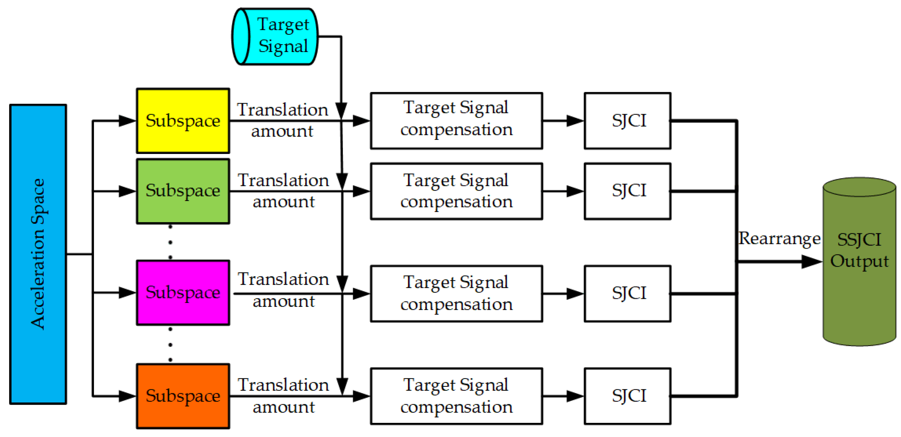
4. SSJCI Algorithm
5. Theoretical Analyses and Performance Comparisons
5.1. Subaperture Time
5.2. SNR Gain
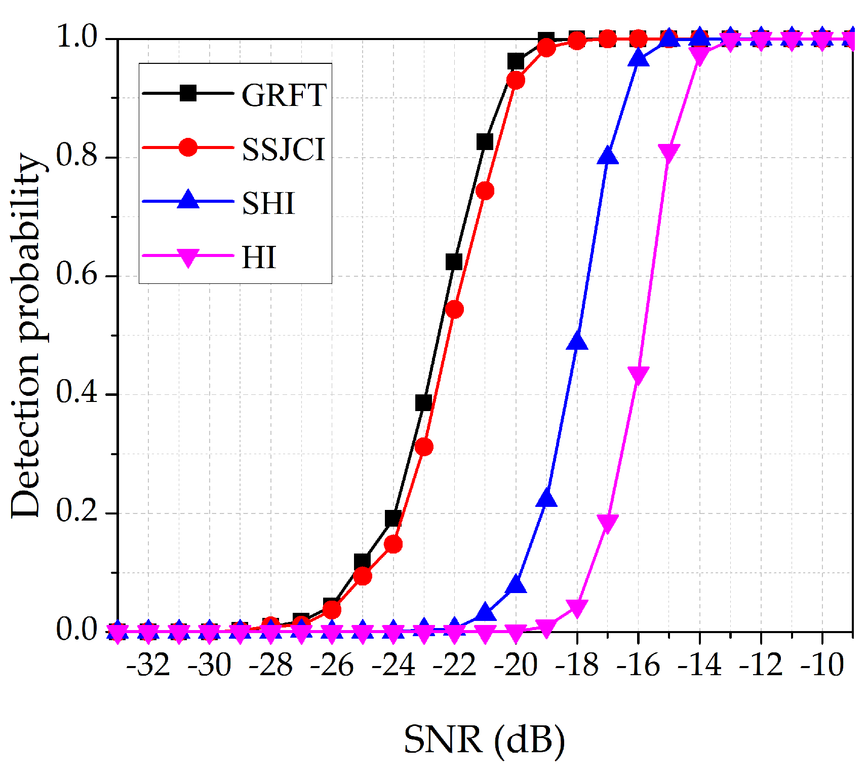
5.3. Detection Probability
5.4. Resolution
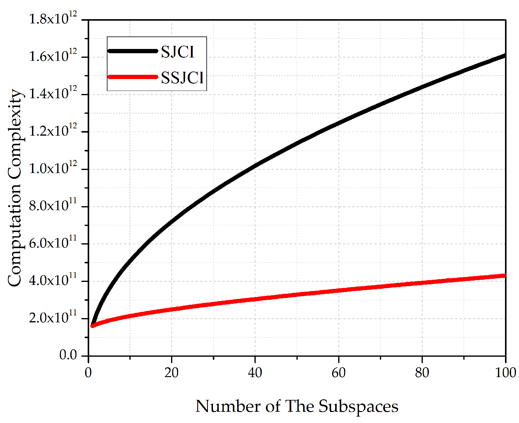
5.5. Computation Complexity
6. Numerical Experiments and Results Analyses
6.1. Multiple Targets Detection
6.2. Detection Performance Comparison
6.3. Real Measured Data Processing
7. Conclusions
Author Contributions
Funding
Conflicts of Interest
References
- Zhu, S.; Liao, G.; Yang, D.; Tao, H. A New Method for Radar High-Speed Maneuvering Weak Target Detection and Imaging. IEEE Geosci. Remote Sens. Lett. 2014, 11, 1175–1179. [Google Scholar]
- Kong, L.; Li, X.; Cui, G.; Yi, W.; Yang, Y. Coherent Integration Algorithm for a Maneuvering Target With High-Order Range Migration. IEEE Trans. Signal Process. 2015, 63, 4474–4486. [Google Scholar] [CrossRef]
- Zheng, J.; Su, T.; Zhu, W.; He, X.; Liu, Q. Radar High-Speed Target Detection Based on the Scaled Inverse Fourier Transform. IEEE J. Sel. Top. Appl. Earth Obs. Remote Sens. 2015, 8, 1108–1119. [Google Scholar] [CrossRef]
- Zheng, J.; Su, T.; Liu, H.; Liao, G.; Liu, Z.; Liu, Q. Radar High-Speed Target Detection Based on the Frequency-Domain Deramp-Keystone Transform. IEEE J. Sel. Top. Appl. Earth Obs. Remote Sens. 2016, 9, 285–294. [Google Scholar] [CrossRef]
- Zhan, M.; Huang, P.; Liu, X.; Liao, G.; Zhang, Z.; Wang, Z.; Hou, Q. Space Maneuvering Target Integration Detection and Parameter Estimation for a Spaceborne Radar System With Target Doppler Aliasing. IEEE J. Sel. Top. Appl. Earth Obs. Remote Sens. 2020, 13, 3579–3594. [Google Scholar] [CrossRef]
- Tian, M.; Liao, G.; Zhu, S.; Liu, Y.; He, X.; Li, Y. Long-time coherent integration and motion parameters estimation of radar moving target with unknown entry/departure time based on SAF-WLVT. Digit. Signal Process. 2020, 107, 102854. [Google Scholar] [CrossRef]
- Rao, X.; Tao, H.; Xie, J.; Su, J.; Li, W. Long-time coherent integration detection of weak manoeuvring target via integration algorithm, improved axis rotation discrete chirp-Fourier transform. IET Radar Sonar Navigat. 2015, 9, 917–926. [Google Scholar] [CrossRef]
- Huang, P.; Liao, G.; Yang, Z.; Xia, X.; Ma, J.; Ma, J. Maneuvering Target Detection and High-Order Motion Parameter Estimation Based on Keystone Transform. IEEE Trans. Signal Process. 2016, 64, 4013–4026. [Google Scholar] [CrossRef]
- Su, J.; Tao, H.; Xie, J.; Rao, X.; Guo, X. Imaging and Doppler parameter estimation for maneuvering target using axis mapping based coherently integrated cubic phase function. Digit. Signal Process. 2017, 62, 112–124. [Google Scholar] [CrossRef]
- Zhang, J.; Su, T.; Zheng, J.; He, X. Novel Fast Coherent Detection Algorithm for Radar Maneuvering Target With Jerk Motion. IEEE J. Sel. Top. Appl. Earth Obs. Remote Sens. 2017, 10, 1792–1803. [Google Scholar] [CrossRef]
- Zheng, J.; Zhang, J.; Xu, S.; Liu, H.; Liu, Q. Radar Detection and Motion Parameters Estimation of Maneuvering Target Based on the Extended Keystone Transform. IEEE Access 2018, 6, 76060–76074. [Google Scholar] [CrossRef]
- Huang, P.; Xia, X.; Liao, G.; Yang, Z.; Zhang, Y. Long-Time Coherent Integration Algorithm for Radar Maneuvering Weak Target With Acceleration Rate. IEEE Trans. Geosci. Remote Sens. 2019, 57, 3528–3542. [Google Scholar] [CrossRef]
- Zhang, S.; Zeng, T.; Long, T.; Yuan, H. Dim target detection based on keystone transform. In Proceedings of the IEEE International Radar Conference, Arlington, VA, USA, 9–12 May 2005; pp. 889–894. [Google Scholar]
- Zhu, D.; Li, Y.; Zhu, Z. A Keystone Transform Without Interpolation for SAR Ground Moving-Target Imaging. IEEE Geosci. Remote Sens. Lett. 2007, 4, 18–22. [Google Scholar] [CrossRef]
- Rao, X.; Tao, H.; Su, J.; Guo, X.; Zhang, J. Axis rotation MTD algorithm for weak target detection. Digit. Signal Process. 2014, 26, 81–86. [Google Scholar] [CrossRef]
- Rao, X.; Zhong, T.; Tao, H.; Xie, J.; Su, J. Improved axis rotation MTD algorithm and its analysis. Multidimens. Syst. Signal Process. 2019, 30, 885–902. [Google Scholar] [CrossRef]
- Xu, J.; Yu, J.; Peng, Y.; Xia, X. Radon-Fourier Transform for Radar Target Detection, I: Generalized Doppler Filter Bank. IEEE Trans. Aerosp. Electron. Syst. 2011, 47, 1186–1202. [Google Scholar] [CrossRef]
- Xu, J.; Yu, J.; Peng, Y.; Xia, X. Radon-Fourier Transform for Radar Target Detection (II): Blind Speed Sidelobe Suppression. IEEE Trans. Aerosp. Electron. Syst. 2011, 47, 2473–2489. [Google Scholar] [CrossRef]
- Xu, J.; Yu, J.; Peng, Y.; Xia, X. Radon-Fourier Transform for Radar Target Detection (III): Optimality and Fast Implementations. IEEE Trans. Aerosp. Electron. Syst. 2012, 48, 991–1004. [Google Scholar]
- Li, J.; Liu, G.; Jiang, N.; Stoica, P. Moving Target Feature Extraction for Airborne High-Range Resolution Phased-Array Radar. IEEE Trans. Signal Process. 2001, 49, 277–289. [Google Scholar]
- Addabbo, P.; Orlando, D.; Ricci, G. Adaptive Radar Detection of Dim Moving Targets in Presence of Range Migration. IEEE Signal Process. Lett. 2019, 26, 1461–1465. [Google Scholar] [CrossRef]
- Shen, Y.; Xu, Y. Analysis of the Code Phase Migration and Doppler Frequency Migration Effects in the Coherent Integration of Direct-Sequence Spread-Spectrum Signals. IEEE Access 2019, 7, 26581–26594. [Google Scholar] [CrossRef]
- Guan, J.; Chen, X.; Huang, Y.; He, Y. Adaptive fractional Fourier transform-based detection algorithm for moving target in heavy sea clutter. IET Radar Sonar Navigat. 2012, 6, 389–401. [Google Scholar] [CrossRef]
- Lv, X.; Bi, G.; Wang, C.; Xing, M. Lv’s Distribution: Principle, Implementation, Properties, and Performance. IEEE Trans. Signal Process. 2011, 59, 3576–3591. [Google Scholar] [CrossRef]
- Tian, J.; Cui, W.; Wu, S. A Novel Method for Parameter Estimation of Space Moving Targets. IEEE Geosci. Remote Sens. Lett. 2014, 11, 389–393. [Google Scholar] [CrossRef]
- Rao, X.; Tao, H.; Su, J.; Xie, J.; Zhang, X. Detection of Constant Radial Acceleration Weak Target Via IAR-FRFT. IEEE Trans. Aerosp. Electron. Syst. 2015, 51, 3242–3253. [Google Scholar] [CrossRef]
- Xu, J.; Xia, X.; Peng, S.; Yu, J.; Peng, Y.; Qian, L. Radar Maneuvering Target Motion Estimation Based on Generalized Radon-Fourier Transform. IEEE Trans. Signal Process. 2012, 60, 6190–6201. [Google Scholar]
- Chen, X.; Guan, J.; Liu, N.; He, Y. Maneuvering Target Detection via Radon-Fractional Fourier Transform-Based Long-Time Coherent Integration. IEEE Trans. Signal Process. 2014, 62, 939–953. [Google Scholar] [CrossRef]
- Li, X.; Cui, G.; Yi, W.; Kong, L. Coherent Integration for Maneuvering Target Detection Based on Radon-Lv’s Distribution. IEEE Signal Process. Lett. 2015, 22, 1467–1471. [Google Scholar] [CrossRef]
- Li, X.; Cui, G.; Yi, W.; Kong, L. A Fast Maneuvering Target Motion Parameters Estimation Algorithm Based on ACCF. IEEE Signal Process. Lett. 2015, 22, 270–274. [Google Scholar] [CrossRef]
- Zheng, J.; Liu, H.; Liu, J.; Du, X.; Liu, Q. Radar High-Speed Maneuvering Target Detection Based on Three-Dimensional Scaled Transform. IEEE J. Sel. Top. Appl. Earth Obs. Remote Sens. 2018, 11, 2821–2833. [Google Scholar] [CrossRef]
- Zhao, L.; Tao, H.; Chen, W. Maneuvering Target Detection Based on Three-Dimensional Coherent Integration. IEEE Access 2020, 8, 188321–188334. [Google Scholar] [CrossRef]
- Xu, J.; Zhou, X.; Qian, L.; Xia, X.; Long, T. Hybrid Integration for Highly Maneuvering Radar Target Detection Based on Generalized Radon-Fourier Transform. IEEE Trans. Aerosp. Electron. Syst. 2016, 52, 2554–2561. [Google Scholar] [CrossRef]
- Ding, Z.; You, P.; Qian, L.; Zhou, X.; Liu, S.; Long, T. A Subspace Hybrid Integration Method for High-Speed and Maneuvering Target Detection. IEEE Trans. Aerosp. Electron. Syst. 2020, 56, 630–644. [Google Scholar] [CrossRef]
- Shidman, D.A. Radar Detection Probabilities and Their Calculation. IEEE Trans. Aerosp. Electron. Syst. 1995, 31, 928–950. [Google Scholar] [CrossRef]
- You, P.; Xu, J.; Qian, L.; Zhou, X.; Xia, X.; Long, T.; Bian, M. Parameter Resolutions of Uniformly Accelerated Targets Based on Hybrid Integration. In Proceedings of the 2016 CIE International Conference on Radar (RADAR), Guangzhou, China, 10–13 October 2016; pp. 1–5. [Google Scholar]


| Procedure | Computation Cost |
|---|---|
| Doppler ambiguity compensation | |
| SFT operation | |
| Phase compensation | |
| Complex addition operation | |
| IFT operation |
| Procedure | Computation Cost |
|---|---|
| ST compensation | |
| SJCI operation |
| Method | Computation Cost |
|---|---|
| HI | |
| SHI | |
| SJCI | |
| SSJCI | |
| GRFT |
| Target | Range () | Velocity () | Acceleration () | SNR () |
|---|---|---|---|---|
| Target A | 5000 | 540 | 54 | −10 |
| Target B | 5000 | 540 | 45 | −10 |
| Target C | 5000 | 630 | 45 | −10 |
| Target D | 5450 | 540 | 45 | −10 |
| Algorithm | HI | SHI | SSJCI | GRFT |
|---|---|---|---|---|
| Required false alarm probability |
Publisher’s Note: MDPI stays neutral with regard to jurisdictional claims in published maps and institutional affiliations. |
© 2021 by the authors. Licensee MDPI, Basel, Switzerland. This article is an open access article distributed under the terms and conditions of the Creative Commons Attribution (CC BY) license (https://creativecommons.org/licenses/by/4.0/).
Share and Cite
Zhao, L.; Tao, H.; Chen, W.; Song, D. Maneuvering Target Detection Based on Subspace Subaperture Joint Coherent Integration. Remote Sens. 2021, 13, 1948. https://doi.org/10.3390/rs13101948
Zhao L, Tao H, Chen W, Song D. Maneuvering Target Detection Based on Subspace Subaperture Joint Coherent Integration. Remote Sensing. 2021; 13(10):1948. https://doi.org/10.3390/rs13101948
Chicago/Turabian StyleZhao, Langxu, Haihong Tao, Weijia Chen, and Dawei Song. 2021. "Maneuvering Target Detection Based on Subspace Subaperture Joint Coherent Integration" Remote Sensing 13, no. 10: 1948. https://doi.org/10.3390/rs13101948
APA StyleZhao, L., Tao, H., Chen, W., & Song, D. (2021). Maneuvering Target Detection Based on Subspace Subaperture Joint Coherent Integration. Remote Sensing, 13(10), 1948. https://doi.org/10.3390/rs13101948