Article

Local- and Regional-Scale Forcing of Glacier Mass Balance Changes in the Swiss Alps

1
Department of Chemistry and Geosciences, Jacksonville State University, Jacksonville, AL 36265, USA
2
International Arctic Research Center, University of Alaska Fairbanks, Fairbanks, AK 99775, USA
3
Department of Geography, Texas State University, San Marcos, TX 78666, USA
4
School of Geosciences, University of Aberdeen, Meston Building, King’s College, Aberdeen AB24 3UE, UK
5
ILR School, Cornell University, 617 Main Street, Suite 300, Buffalo, NY 14203, USA
*
Author to whom correspondence should be addressed.
Remote Sens. 2021, 13(10), 1949; https://doi.org/10.3390/rs13101949
Submission received: 8 March 2021 / Revised: 22 April 2021 / Accepted: 11 May 2021 / Published: 17 May 2021
(This article belongs to the Special Issue Applications of Remote Sensing in Glaciology)

Abstract

:
Glacier mass variations are climate indicators. Therefore, it is essential to examine both winter and summer mass balance variability over a long period of time to address climate-related ice mass fluctuations. In this study, we analyze glacier mass balance components and hypsometric characteristics with respect to their interactions with local meteorological variables and remote large-scale atmospheric and oceanic patterns. The results show that all selected glaciers have lost their equilibrium condition in recent decades, with persistent negative annual mass balance trends and decreasing accumulation area ratios (AARs), accompanied by increasing air temperatures of ≥ +0.45 °C decade−1. The controlling factor of annual mass balance is mainly attributed to summer mass losses, which are correlated with (warming) June to September air temperatures. In addition, the interannual variability of summer and winter mass balances is primarily associated to the Atlantic Multidecadal Oscillation (AMO), Greenland Blocking Index (GBI), and East Atlantic (EA) teleconnections. Although climate parameters are playing a significant role in determining the glacier mass balance in the region, the observed correlations and mass balance trends are in agreement with the hypsometric distribution and morphology of the glaciers. The analysis of decadal frontal retreat using Landsat images from 1984 to 2014 also supports the findings of this research, highlighting the impact of lake formation at terminus areas on rapid glacier retreat and mass loss in the Swiss Alps.

Graphical Abstract

1. Introduction

Glacier mass balance, the difference between accumulation and ablation, is an important prerequisite for monitoring direct and immediate impacts of climate forcing on the cryosphere [1]. Glaciers react to climatic conditions by losing or gaining mass [2,3,4]. This reaction is mainly controlled by two processes: snowfall precipitation within the accumulation zone in winter and snow–ice melt, runoff, and sublimation during the summer. In connection with ongoing global atmospheric warming and rising air temperatures, the ablation season has expanded and resulted in the acceleration of glacier volume loss [2,5]. Therefore, changes in seasonal mass balance can be considered a clear indicator of climatic variations in high-mountain regions [6]. Since glacier mass balance is linked directly to local meteorological conditions and large-scale atmospheric circulation, as well as glacier dynamics and hydrology, a thorough understanding of glacier mass balance and its interactions with climatic variables is critical to local communities and regions because of hydropower supply [7,8,9,10,11,12], irrigation systems [13,14], hazard monitoring [15,16,17,18], and opportunities like geotourism [19,20,21,22].
There is a long-standing tradition of measurements of European glacier’s surface mass balance conditions. The first mass balance concepts involved a series of accumulation and ablation measurements on Nordic glaciers in the 1920s and 1930s [23]. However, glacier monitoring started in 1894 with a more simplified focus on glacier length changes [24]. After the late 1940s, interests were shifted to collecting data on glacier-wide mass balance [25]. The first standardized data publication on change in glacier length, area, volume, and mass started with the ‘Fluctuations of Glaciers’ series in the late 1960s [2,26]. Since the 1980s, data on glacial changes has been documented in a relational database, Worldwide Glacier Monitoring, for access by scientists, policy makers, and the public [2,27]. The World Glacier Monitoring Service (WGMS) plays a critical role by compiling available data through a scientific and international network based on contributions from thousands of observers from all over the world. These archives are based on common measurement protocols and are currently available through the WGMS and Global Terrestrial Network for Glaciers (GTNG) as part of the Global Climate Observing System. Mass balance data are obtained either from direct glaciological methods (field measurements) or from satellite/aerial monitoring change on glacier surface topography, which converts the volume to mass change using a density assumption [28,29].
Compared to other mountain ranges around the world, the European Alps have the longest record of mass balance data [23]. According to available reports and previous studies, these glaciers have demonstrated great mass loss since the Little Ice Age. Zemp et al. [30] modeled glacier mass balance fluctuations for the European Alps dating back to 1850 using the inventory from the WGMS and the Swiss Glacier Inventory of 2000. They reported an overall estimated loss of 35% in glaciated areas from 1850 to the 1970s, followed by a 50% acceleration in mass loss from 1970s to 2000, visible mainly as terminus retreat. It has been suggested that such fluctuations in glaciers are the indirect and lagged response to past climatic conditions [2,31,32]. Huss et al. [31] re-analyzed seasonal glacier-wide mass balance in the southeastern Swiss Alps from 1900 to 2008 based on field measurements. Using a distributed accumulation and temperature-index model, the authors concluded that the rate of mass loss in this time frame varied significantly between adjacent glaciers because of the dynamic adjustment to the post-Little Ice Age climate change, namely warm air temperatures. Their study also projected a 63% decrease in glacier extent through 2050 and increased annual runoff over the next three decades for the deglaciating catchments. Fischer et al. [1] extended a re-evaluated inventory of geodetic mass balance, surface elevation change, and volume change for the entire glaciers in the Swiss Alps from 1980 to 2010. The estimated average mass balance was −0.62 ± 0.07 m w.e. yr−1, with an overall volume loss of −22.51 ± 1.76 km3. The findings of this research also revealed the mass change for the glaciers in Valais Alps (Rhone) to be lesser (−0.59 m w.e. yr−1), and that for the southern glaciers (e.g., Maggia, Ticino, Maira, Poschiavino) to be greater, than that for the entire Swiss Alps. Following that study, Huss et al. [33] re-evaluated 19 series of the Swiss glacier-wide seasonal mass balance from 1920 based on point observations to establish a homogenous mass balance series. This dataset, which includes winter (1 October–30 April) and summer (1 May–30 September) observations back to the 1980s, offers a strong basis for analyzing the response of glacier mass balance components to climate variability and change.
Previously, numerous studies have addressed the sensitivity of mass balance to various climatic factors including changes in surface air temperature and precipitation [3,34,35,36,37,38,39]. Huss and Fischer [40] developed a model, the Glacier Evolution Runoff, to evaluate the response of very small glaciers (<0.5 km2) in Switzerland to current and future atmospheric warming. According to their study, Swiss glaciers are projected to disappear in the next 25 years. Glacier mass balance, in general, has also been linked to oceanic and atmospheric variability through various climate indices (e.g., the North Atlantic Oscillation (NAO), the East Atlantic (EA) pattern, and the Atlantic Multidecadal Oscillation (AMO)) [3,41,42,43,44]. The impact of such climate forcing on Swiss glaciers have been addressed in a few studies [6,32,45]. Huss et al. [32] associated North Atlantic climate variability with the 100-year surface mass balance record for thirty Swiss glaciers. The results found the AMO index inversely correlated with glacier mass balance, suggesting that positive AMO values (warm sea surface temperatures) impacted significant mass loss from 1908 to 2008.
Even with a rich literature dedicated to monitoring long-term glacier trends, there is still a further need to perform time series analysis to quantify Swiss glacier mass balance changes and drivers as they relate to local and remote climatic conditions, specifically for glaciers included in newly developed datasets [33]. Moreover, there is a special need to study the development and evolution of catchments through ice melt and associated features such as new lakes, since they are closely tied to glacier ice loss [46]. As such, our study employed glaciological, remote sensing, and climate datasets and assessed glacier mass balance components and hypsometric characteristics with respect to interactions with local meteorological variables and remote large-scale atmospheric and oceanic patterns to more comprehensively understand physical processes driving glacier mass balance variability.
Precisely, we analyzed the behaviors of the southwestern Swiss glaciers in the context of post-Little Ice Age climate change. We also conducted a long-term (1970–2017) time series analysis of annual glacier mass balance (1 October–30 September), as well as winter (1 October–30 April) and summer (1 May–30 September) mass balances, derived from glaciological reports (1881–2014) contained in the WGMS [26]. Additionally, we analyzed and compared the time series data to identify trends, fluctuations, and similarities in glacier annual and seasonal mass balances. We further provided hypsometric characteristics of these glaciers using swissALTI3D Digital Elevation Model (DEM) and Advanced Spaceborne Thermal Emission and Reflection Radiometer (ASTER) Global DEM (GDEM) Version 3 (V3) and examined the possible impacts of geometry on the recorded responses. Using Landsat satellite images covering a span of 30 years, we investigated the changes in the rate of terminus retreat for these glaciers. We further explored impacts of local climatic variations, including the air temperature fluctuations during ablation season (May–September) and precipitation during accumulation season (October–April). We then evaluated multidecadal variations of glacier mass balance and local climate to forcing from regional atmosphere–ocean patterns, including the AMO, NAO, and EA, as well as the Scandinavian pattern (SCA) and Greenland Blocking (described by the Greenland Blocking Index (GBI)), since the atmospheric patterns described by these indices play a key role in modulating European weather and climate [47].

2. Study Area

This study is focused on seven glaciers (Grosser Aletschgletscher, Allalin, Hohlaub, Schwarzberg, Gries, Gietro, and Rhone) of varying size, geometry, hypsometry, aspect, and slope, in the Upper Rhone catchment (Figure 1 and Table 1). Grosser Aletschgletscher, which is located within the Bernese Alps, is the longest (22.6 km) and largest (83.0 km2) ice body in the European Alps, with an extensive archive of climate data and glaciological records dating back to 1841 [22,48]. The accumulation area of this glacier faces south and contains two summits, Jungfrau and Mönch. The main body is divided by three branches (Grosser Aletschfirn, Jungfraufirn, and Ewig Schneefeld) at Konkordiaplatz with reported ice thickness of 890 m at its summit. According to the reports, it has lost significant volume since the Little Ice Age with a fast acceleration since the late 1980s [26].
Rhone is a south-facing valley glacier with a climatic condition similar to Aletsch. Gries is different in this regard than the other glaciers as it is placed south of the main Alpine crest at the border of Italy within a small valley exposed in a northeastern direction with relatively high precipitation. According to Huss et al. [6], Gries and Aletsch have lost 39% and 16% of their ice volume in the 20th century, respectively. Mass balance monitoring programs were established on Gries in the 1960s with hydropower projects, whereas the data collections on Aletsch and Rhone were taken as a part of glaciological research projects.
The Mattmark region includes three glaciers (Allalin, Hohlaub, Schwarzberg), with the longest mass balance record dating back to 1955, established during the construction of Mattmark dam in the Saas Valley. The Laboratory of Hydraulics, Hydrology, and Glaciology at ETH Zürich (VAW/ETHZ) has been observing the glaciers in corresponding catchments, including Gietro and two other glaciers, Allalin and Schwarzberg, in the Mattmark area (Saastal). Allalin is a large valley glacier flowing in a northeast direction and covers 9.6 km2 of the Saas Valley. This glacier has the highest equilibrium line altitude (ELA) of 3575 m a.s.l. owing to the little solid precipitation in the valley [26]. According to the Swiss glaciers report in 2014/2015, the least amount of mass loss, relative to the inventory, was recorded for this glacier, with average thickness changes of approximately −0.6 m w.e. [26].
Two additional glaciers, Silvretta and Clariden, located outside of the catchment in the Central and Glarus Alps, respectively, have the longest records in the Swiss glacier database since the 1900s, and are included to understand the regional variations between the glaciers and provide information on the temporal and spatial patterns of mass balance fluctuations within the Swiss Alps. The glaciers vary in size from 2 to 83 km2 as documented by VAW/ETHZ glaciological reports (1881–2014), which includes stake-derived mass balance measurements as well as geometries, aspects, and local climatic conditions of individual glaciers.

3. Data

A wealth of data is available for the Swiss glaciers, especially in the Upper Rhone catchment. The combination of mass balance measurements (Table 1) and climate data allows us to draw an integrative picture of the local and regional forcing of mass balance variations in this region.

3.1. Mass Balance Data

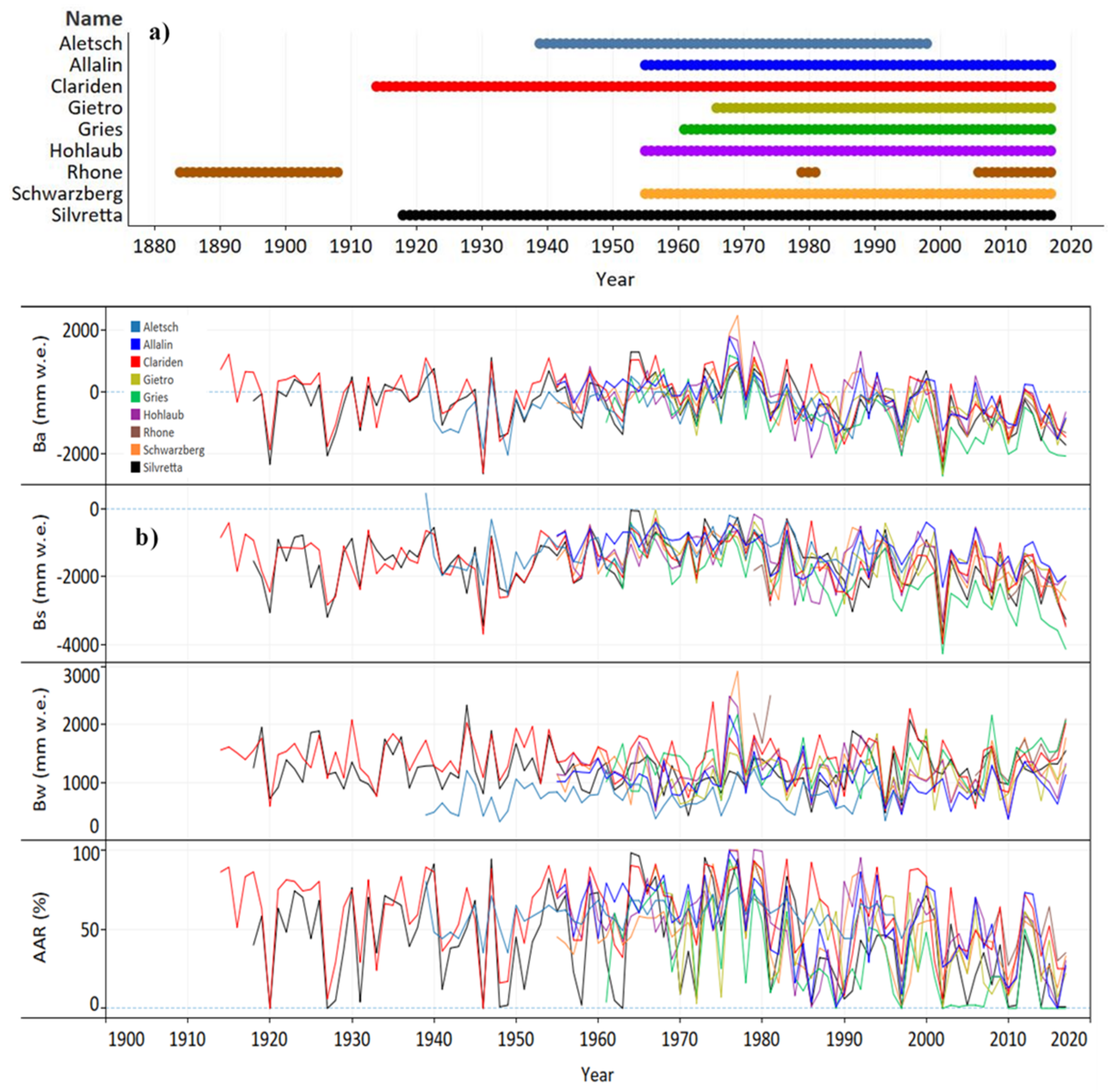
For the Swiss Alps, two direct mass balance series are available that span five continuous decades (Table 1, Figure 2) [26,33].
These mass balance time series are calculated by glaciological field methods including dense snow probings and pits dug in April–May that measured the winter snow accumulation, and ablation stake readings in September [40]. The longest mass balance time series (since 1900) for 50 glaciers in the Swiss Alps was reconstructed by Huss et al. [33] based on the combination of field measurements and ice volume changes by comparison of DEMs. The extrapolation of individual measurements to the entire glacier surface was performed using a mass balance model which considers all important processes controlling glacier mass balance distribution. There are seven glaciers in the Upper Rhone catchment with a long sequence of mass balance measurements recorded since 1884. In this dataset, winter mass balance (Bw), corresponds to the accumulated snow/ice mass measured from October to the end of April. Summer mass balance (Bs) is the result of difference between annual mass balance (Ba) determined at the end of the ablation period (end of September) and Bw. The length of annual mass balance and time series of Ba, Bw, Bs, and AAR for each glacier are presented in Table 1 and Figure 2a,b.

3.2. Climate Data

Monthly mean air temperature and precipitation data are used to determine the relationship between the mass balance components and local climate. Long-term homogenized series of average daily air temperatures (two meters above surface) and total precipitation from the Swiss National Basic Climatological Network (NBCN) stations considering the underlying topography, with coverage since 1961 over the entire Swiss Alps, were provided by MeteoSwiss in a 2 × 2 km grid structure [49,50]. The daily mean meteorological time series is extracted from the gridded area covering the glaciers.
In order to assess the relationship between the components of mass balance and the larger-scale atmosphere and oceanic conditions, seasonal (October–April and May–September) and annual times series of the NAO, SCA, and EA were obtained from the Climatic Prediction Center (CPC), and those of the GBI [44] and AMO were downloaded from the National Oceanic and Atmospheric Administration (NOAA). The GBI represents the normalized 500 hPa mean GPH anomalies across Greenland, 60–80° N, 20–80° W [51,52,53,54]. The NAO has been defined in several ways, and we use two versions here. The Hurrell NAO index used here is based on an empirical orthogonal function (EOF) analysis of North Atlantic sea-level pressure, which tends to capture spatial variations in the action centers generally found over Iceland and the Azores [55]. To evaluate the upper-air circulation features over a similar geographic area, the CPC NAO index is used supplementally and is identified as the first EOF derived from a rotated EOF analysis of 500 hPa anomalies from 20–90° N. The corresponding second and third EOFs, the EA and SCA, are also analyzed to understand a broader array of North Atlantic synoptic settings potentially linked to the Swiss glaciers variability and changes. The EA pattern tends to have an action center near 80° N and 20–35° W, while the SCA coincides with a high-pressure center over the Scandinavian countries during its positive phase [56,57]. The AMO index used here is based on detrended North Atlantic sea surface temperature anomalies from the Kaplan SST dataset [58,59]. This teleconnection is linked to continental climate variations in both North America and Europe [58]. Positive AMO values are associated with warm near-surface air temperature anomalies in Europe, and prevailing low-pressure anomalies over the Atlantic and Europe during the winter (DJF) [60].

3.3. Remotely Sensed Data

For hypsometric analysis, we use swissALTI3D DEM obtained from the Swiss Federal Office of Topography (Swisstopo) for the seven glaciers in the catchment and the newly released ASTER GDEM Version 3 (V3) data for the two additional glaciers located in the Central and Glarus Alps. This swissALTI3D DEM (2019 edition) represents the surface glaciers at a spatial resolution of 10 m with ±1 m to 3 m (1σ) vertical accuracy for the stereo correlation and ±0.1 m to 1 m for manual stereo measurements. Areas below 2000 m a.s.l. were created using airborne laser scanning data with an accuracy of ±0.5 m (1σ) [61]. The ASTER GDEM V3 was released in 2019 and displays similar level of accuracy as ASTER GDEM V2. However, V3 has lesser void area due to the increase in ASTER stereo image data since the previous release and improved processing [62].
To observe the glacier termini changes over a period of three decades (1984–2014), we use 12 Landsat 5 Thematic Mapper (TM) and Landsat 8 Operational Land Imager (OLI) images downloaded from EarthExplorer data portal [63]. The images are selected if they are completely cloud-free over the termini of the glaciers and show least seasonal snow cover for the selected timeframe. The collected images are then spread across a 10-year time interval, except for Gietro (Table 2), due to the unavailability of cloud-free coverage of its terminus within the same years as for other glaciers.

4. Methods

To achieve the research objectives, we adopted a coherent approach combining statistical methods for glaciological and climate time series with geospatial methods for remote sensing data (Landsat and DEM) analyses to make meaningful inferences. Below, we have compiled the methods within various sub-sections to detail on the key steps for any such analyses in future works.

4.1. Statistical Analysis

4.1.1. Exploratory Data Analysis

Using the WGMS database, time series of Ba, Bw, Bs, and AAR (the ratio of accumulation area at the end of melt season to total glacier area) are calculated and assessed for inhomogeneities (i.e., missing values (Figure 2), and any change in unit measurements), testing assumptions to select the analysis strategy (e.g., presence of autocorrelation within the time series), trends and outliers, fluctuations, and the general pattern of glacier behaviors (i.e., mean and standard deviation of Ba, Bs, Bw, and AAR of glaciers) within the common period of observation (1970–2017). Exploratory analyses are initially conducted, including time series plots, boxplots, autocorrelation functions, correlation matrices, and smoothing techniques (i.e., moving averages). To identify similarities between glaciers and address the seasonal aspect of mass balance, the Ba series of all the glaciers are intercompared and linked with Bw and Bs characteristics using Spearman correlation analysis. Prior to conducting correlation analyses, data series are detrended using a triangular moving average approach to detect and highlight intradecadal changes [44,64,65]. A seven year level of triangular average is applied as it yields optimal correlations between the annual and seasonal mass balance of all glaciers versus seasonal and annual climate indices.

4.1.2. Structural Change Model

Various approaches have been developed in the literature for testing structural changes and identifying breakpoints in time series. Most tests examine coefficient changes of a linear regression model where the assumption is a single change in time and the type of change is known [66]. Another method referred to as multiple structural changes has been widely used [66,67,68,69,70] to test the presence of multiple shifts over time. We consider a linear regression model as:
y i = x i T β i + µ i i = 1 , ,   n
where at time   i , y i is the observation of the dependent variable, x i is a k × 1 vector of regressors, and β i is the k × 1 vector of regression coefficients [71]. Here, the null hypothesis is that the regression coefficients are constant, while the alternative hypothesis is that at least one coefficient changes over time:
H 0   : β i   = β 0 i = 1 , ,   n
This assumes that there are m breakpoints, where the coefficients deviate from one stable regression relationship to a different one [66]. Thus, there are m + 1 segments in which the regression coefficients are constant, and model (1) can be rewritten as:
y i = x i T β i + µ i i = i j 1 + 1 , ,   i j   , j = 1 , ,   m + 1
where j is the segment index, and Im,n = {i1, …, im} refers to the set of breakpoints or the number of m partitions [66].
Overall, two approaches for testing structural change are used: (i) F statistics [72], and (ii) generalized fluctuation tests [73]; the former approach tests against a single-shift alternative of unknown timing, whereas the latter technique, also known as empirical fluctuation process (efp), is concerned with constancy in a graphic method reflecting the fluctuations in residuals and coefficient estimates [74]. The null hypothesis of the generalized fluctuation test is based on the central limit theorem, and if the efp boundaries are crossed by fixed probability α, the fluctuation is large, and the null hypothesis of no structural break is rejected. The efp function from the fluctuation test framework was programmed in R and the cumulated sum of standard OLS residuals (CUSUM) function was specified as the type of fluctuation process to be fitted in the argument. CUSUM detects change points in time series that often results from structural changes based on the limiting process of standard Brownian motion [75]. Since the number of breakpoints m is not known in advance, it is necessary to compute the optimal breakpoints for m = 0, 1, …n breaks and choose the model that minimizes some information criterion such as the Bayesian information criterion (BIC) [76]. Following this exercise, a Chow test [77] is also performed to confirm the statistical significance of resulting change points (10-year sliding window) at the 95% confidence level when p ≤ 0.05.

4.1.3. Trend Analysis

Mann–Kendall and Sen’s Slope Estimator

To evaluate whether mass balance values increase or decrease over time, the Mann–Kendall test is applied. This test, which is a nonparametric form of monotonic trend regression analysis, is robust to missing values and outliers in time series. The test assumes that the data are independent, and the distribution of data remains consistent [78]. Therefore, autocorrelation (ACF) and partial autocorrelation (PACF) tests are conducted, and serial correlation is not found in the series which further motivated application of this approach.
The Mann–Kendall test calculates the difference between the later value and all previous values, (xjxi), where j > i, and assigns the value of 1, 0, or −1 to positive, no differences, and negative differences, respectively [79,80]. The test statistic, S, is then calculated as:
S = i = 1 n 1 J = i + 1 n s g n x j x i
where sgn (xj − xi), is equal to +1, 0, or −1. When S is greater than 0, xj > xi, an upward trend is indicated, while negative S values, xj < xi, indicate a downward trend. If xj − xi is 0, trend is not present within the time series. The test statistic τ can be computed as:
τ = S n n 1 / 2
which has a range of −1 to +1 and is analogous to the correlation coefficient in regression analysis. S and τ values that are significantly different from zero indicate the presence of trend and reject the null hypothesis of no trend. Following that, the rate of change or the power of the trend can be obtained using Sen’s slope estimator [78]:
β 1 = median   x j   x i y j   y i
in which the slope of all the pairs is computed and the median of these slopes is denoted.

Multiple Linear Regression

We used multiple linear regression to account for the association of relevant variables including mean summer temperature (May–September) and winter precipitation (October–April), with the annual mass balance response variable. The regression model that is estimated specified annual mass balance (Ba) as a function of time (t), summer temperature (Ts), and winter precipitation (Pw) is as follows:
Ba = β0 + β1 t + β2 Ts + β3 Pw
where β0 is the intercept, ε is the unexplained model error, and β1..3 refers to the slope coefficients of time, summer temperature, and winter precipitation, respectively. The null hypothesis related to time is that the parameter β1 = 0. Rejecting this null hypothesis in favor of a nonzero β1 would indicate a trend. Similarly, the null hypotheses related to parameter β2 and β3 are that both are equal to zero (i.e., no trend). Evidence against these hypotheses (i., β1 > 0) suggests that they are helpful in understanding temporal variation in annual mass balance. If the null hypotheses are not rejected, however, a simple regression model should be applied. The key assumptions in this model include normal distribution of residuals, independent variables, and homoscedasticity, which are tested and satisfied, justifying use of this technique.

4.2. Remotely Sensed Data Analysis

In the following Section 4.2.1 and Section 4.2.2 we use remotely sensed data to link the mass balance analysis and the local and regional climate forces with the hypsometry and decadal frontal retreat of glaciers to confirm the statistical results from the previous sections.

4.2.1. Hypsometric Index (HI) and Hypsometric Integral (HIn)

We use Equation (8) as suggested by Jiskoot et al. [81] to perform the HI calculations.
HI = (Hmax − Hmed)/(Hmed − Hmin), If 0 < HI < 1 then HI = −1 / HI
Here, Hmax and Hmin are the maximum and minimum elevations, respectively, and Hmed is the median elevation. Based on the thresholds suggested by Jiskoot et al. [81], glaciers can be divided into five categories: (1) very top-heavy (HI < −1.5), (2) top-heavy (−1.5 < HI < −1.2), (3) equidimensional (−1.2 < HI < 1.2), (4) bottom-heavy (1.2 < HI < 1.5), and (5) very bottom-heavy (HI > 1.5).
HIn, also known as the ‘elevation–relief ratio’, represents the area under the normalized elevation curve with values between 0 and 1. HIn is widely used in hydrological and geomorphological studies and is calculated using Equation (9) [82,83].
HIn = (Hmean − Hmin)/(Hmax − Hmin)
Here, Hmax and Hmin are the maximum and minimum elevations, respectively; and Hmean is the mean elevation. Low HIn values represent a concave hypsometric curve, whereas larger values depict a convex curve. Both HI and HIn are used to give a better understanding of the erosion and fluvial activity along with the shape of the glacier basin [81,83,84].

4.2.2. Glacier Terminus Delineation

The terminus outlines are delineated manually based on visual observations of temporal Landsat images. The approach defined by Bjørk et al. [85] is adopted for reporting the recession rates, where the ice front is first divided by generating equally spaced points. We then calculate the mean distance between points with respect to a fixed point placed up glacier. To maintain uniformity in this approach related to data spatial resolution, we make all the observations on 30 m Landsat images. We follow the approach suggested by Hall et al. [86] and use Equation (10) to estimate the uncertainty associated with terminus recession rates:
U = ((I1)2+(I2)2)1/2 + Ereg
where U is the total uncertainty in terminus position, I1 is the pixel size of the image from earlier year, I2 is the pixel size of the image from the later year, and Ereg the co-registration error between images. The geo-registration of Landsat Tier 1 scenes is consistent and within prescribed image-to-image tolerances of ≤12 m radial root mean square error (RMSE). Thus, considering 12 m as the Ereg value provides us with a total uncertainty of U~ 54.43 m.

5. Results and Discussion

5.1. Analysis of Annual Mass Balance

Trend calculations on the annual mass balance dataset for the selected glaciers in the Swiss Alps, from the early 1900s to 2017, reveal a negative downward trend and two significant breaks in the 1980s and 2000s (Figure 2b and Table 3). However, the Ba of Gries and Schwarzberg glaciers show three break points. Accordingly, the series of Schwarzberg includes three phases: (i) the years from 1956 to 1970 with a near-equilibrium condition (μBa = −69 mm w.e., σ = 344 mm w.e.), (ii) the period from 1971 to 1980 of mass gain (μBa = 621 mm w.e., σ = 933 mm w.e.), and (iii) the period after 1980 with a strong imbalance due to mass loss (μBa = −640 mm w.e., σ = 650 mm w.e.). Similarly, Gries shows breaks in: (i) the period from 1962 to 1980 with a nearly balanced condition, (ii) from 1981 to 2000 (μBa = −885 mm w.e., σ = 541 mm w.e.), and (iii) a rapid mass loss period from 2001 to 2017 (μBa = −1527 mm w.e., σ = 590 mm w.e.). Among the other glaciers, the rates of change after break years (1980s) become negative for Allalin and Hohlaub. In Gietro and Silvretta, the rates have changed from −200 to −1000 mm w.e., indicating a trajectory toward the disappearance of these glaciers in the near future. Based on these results, we can conclude that the 1970s was a decade of mass gain, and the mid-1980s onward, especially the 2000s and 2010s, have been the decades of rapid mass loss for many of the glaciers in the Swiss Alps. According to [87], the melt extremes of the 2000s occurred under high shortwave irradiance and large downward latent and sensible heat fluxes in association with increased atmospheric moisture content. In contrast, melt events at the end of the 1980s were associated with lower downward turbulent heat fluxes explained by high downward shortwave radiation under relatively dry atmospheric conditions.
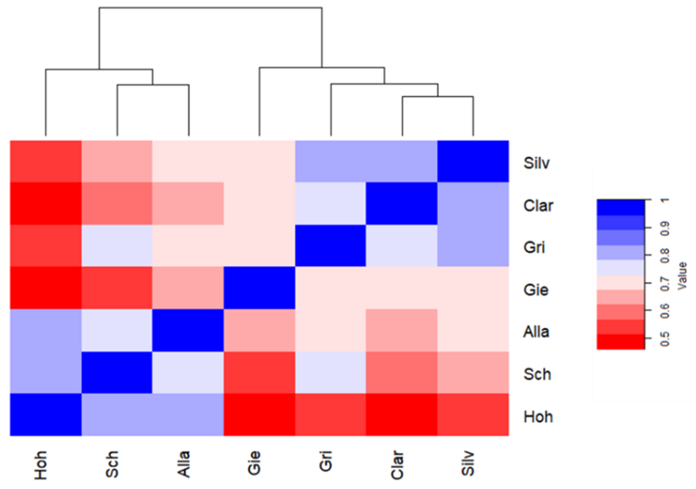
The correlation analysis of glaciers reveals a significant relationship among the Ba of the glaciers (Figure 3). Accordingly, Silvretta, Clariden, Gries, and Gietro can be categorized into one group, and Allalin, Schwarzberg, and Hohlaub in another group. The similarity of Allalin, Schwarzberg, and Hohlaub can be attributed to the proximity of these glaciers and corresponding geomorphic (e.g., elevation range, degree of debris coverage, surface slope, and surface facing) and local climatic factors (e.g., precipitation and temperature).
Although the glaciers in the first group are located apart from each other, they have exhibited similar rapid rates of change in mass balance in the available series. In this group, the size of these glaciers, except Gietro, is less than 5 km2 (see Table 1), which makes them more sensitive to warming air temperatures.

5.2. Analysis of Seasonal Mass Balance and Accumulation Area

The analysis of Bs and Bw suggests that the changes in mass balance are primarily influenced by increases in ablation rates during summer (Table 4), which agrees with previous studies [3,33].
The comparison of summer mass balance and AAR series indicates that the glaciers’ accumulation area has decreased at the expense of increased ablation rates and areas. Among the glaciers, the accumulation area of Gries approached zero from 2000 to 2007 and again from 2014 to 2017. Gries is a medium-sized steep glacier that is faced to the northeast. Unlike Gries, the highest increase in AAR was observed in Clariden, which is likely related to the greater amount of solid precipitation received during the accumulation months. Overall, the accumulation areas of larger glaciers have been more consistent than smaller glaciers. For example, the AAR of Aletsch glacier, the largest of those surveyed, has fluctuated around 50% through the entire period and has been less sensitive to climate variations. The larger glaciers’ state can be explained by their ability to dynamically adjust to climate warming by retreating to higher elevations [33]. Further, the decrease in surface albedo and bare terrain exposure at the terminus coincides with an increase in upward longwave radiation from and downward shortwave absorption to accelerate glacier frontal retreat and melt in the ablation area [33,87].
The time series of glaciers is continuous within the common period of 1970 to 2017 (Figure 2b). With the comparison of glaciers in this period, lower Bs mean and higher Bs variation are observed for Gries with −2232 mm w.e. and 838 mm w.e., respectively. During the accumulation season, glaciers received an average of approximately 1000 mm w.e., with the highest value for Clariden (1385 mm w.e.). In the same period, the lowest average annual mass balances of −919 mm w.e. for Gries and −509 mm w.e. for Silvretta were detected. Similarly, the mean AARs were significantly lower for Gries and Silvretta (26% and 36%) and higher for Clariden (56%). The comparison of seasonal and AAR values indicates that the glaciers like Hohlaub, Allalin, and Schwarzberg are roughly in equilibrium relative to other glaciers due to higher altitudinal ranges. Switzerland’s air temperatures are highly dependent on elevation, and much of the observed warming has been found at lower elevations due to increased incoming shortwave radiation under more frequent anticyclonic conditions [88].

5.3. Climatic Controls

5.3.1. Local Meteorological Variables

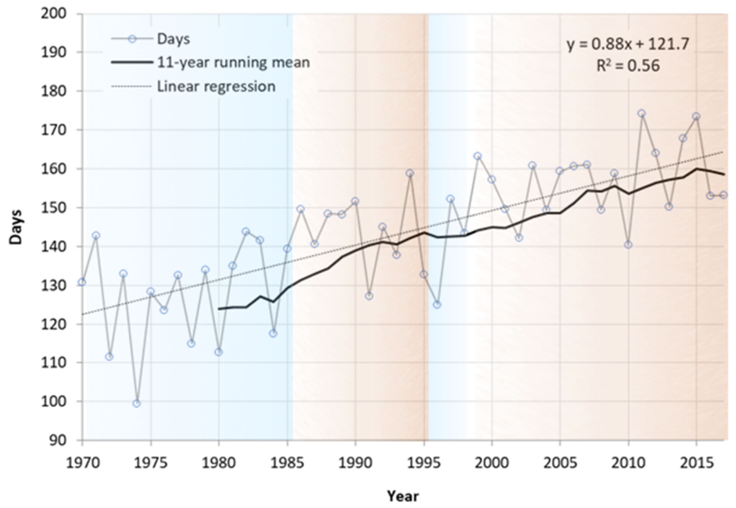
The overall analysis of days with the maximum temperature > 0 °C per year for all selected glaciers indicates that the total number of days has considerably increased from 130 days in 1970 to 175 in 2015 with a change rate of ~9 days per decade (Figure 4).
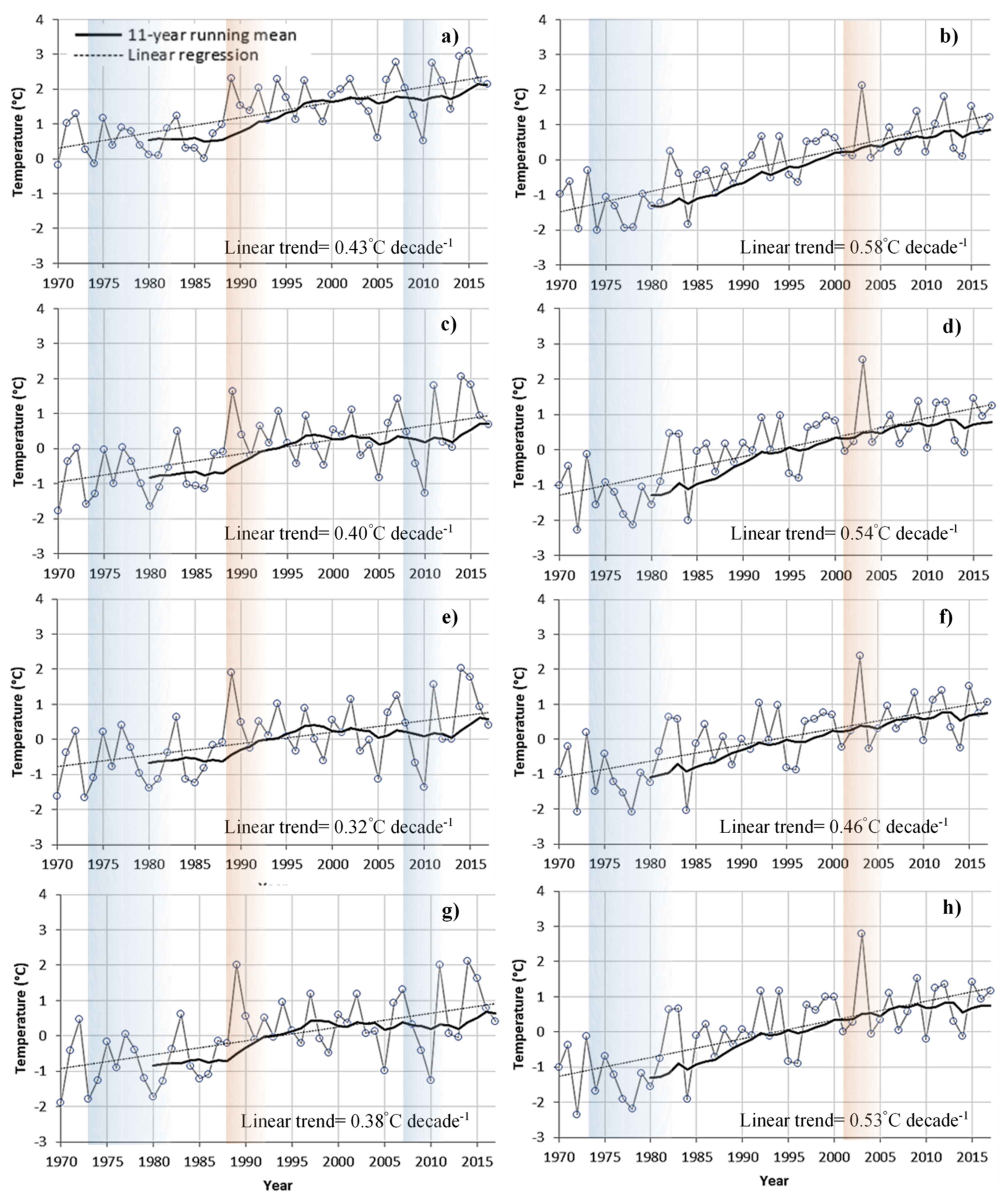
The strongest summer warming trends were during the period of 1970 to 2017 (Figure 5b,d,f,h). The largest trends were found for glaciers located in the southern Rhone including Gietro, Hohlaub, Allalin, and Schwarzberg (0.58 °C decade−1) (Figure 5b), and the smallest trend was found for for Silvretta (0.46 °C decade−1) (Figure 5f). Following the same pattern of the Italian Alps [3], three discernible phases can be detected from a 11-year running mean applied to the time series. The first phase starts from 1970 with the mean air temperature anomalies around −1 °C. Then, after 1985, the anomalies reached 0 °C and remained stable until 2000s. Since the 2000s, air temperature anomalies over glaciers have been accelerating beyond 0 °C and have approached +1 °C in recent years with the unprecedented peak of roughly +3 °C for all glaciers in 2003.
The warming trends during the winter season vary from 0.32 to 0.43 °C decade−1, with the lowest trend associated with Silvretta and the highest to the southern Rhone glaciers. The fluctuations in temperature values over the selected period were different for the glaciers located in southern Rhone during the accumulation season. The corresponding moving averages show that the positive trend lasted up to 1985, then gradually declined for five years until it reached 0–1 °C above average in 1990s. Over the 2010s, the temperature anomalies of this group of glaciers oscillated between +2 and +3 °C during the winter months. The warmest peaks of these glaciers happened in 1989 and 2014/2015, whereas a dramatic drop (below 1 °C for the southern glaciers and below −1 °C for other groups) occurred in 2010. Despite the dissimilarity of Silvretta and Clariden during summer (Figure 5f,h), the temperature trends are quite similar during the accumulation season.
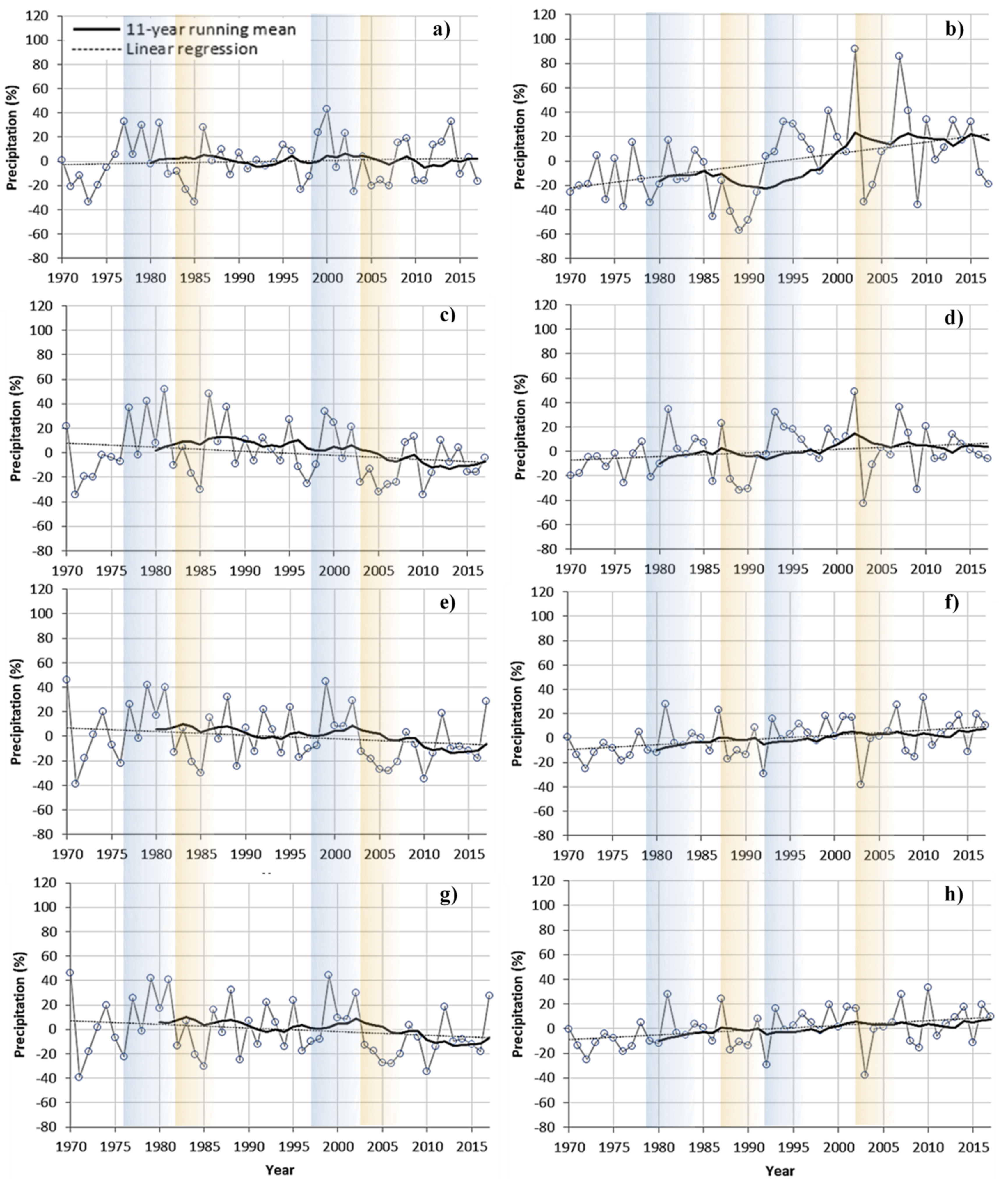
The total precipitation anomalies do not reveal significant trends in accumulation season (Figure 6a,c,e,g). The moving averages of precipitation have fluctuated close to the long-term mean. However, for the northern Rhone glaciers (Figure 6c), Silvretta (Figure 6e), and Clariden (Figure 6g), two phases are apparent. In the first phase, periods with above-average precipitation were frequent prior to the second half of the 2000s, with the maximum of ≈40% and the minimum of ≈−40% in 1985 and 2005 and the maximum of 50% at the beginning of the 1980s. In the second phase, running average precipitation remained steady prior to 2010 and was then followed by a ≈10% drop below the long-term mean after 2010.
Precipitation during the ablation season showed a slightly different pattern (Figure 6b,d,f,h), especially for the glaciers located in the southern Rhone (Figure 6b). This group of glaciers has experienced an upward trend over the selected period, including three phases as highlighted by the moving average. The period of the 1970s and the first half of the 1980s with precipitation 10% below the average was followed by a drastic drop to 20% below average that lasted for 20–25 years. From 2000 to 2015, only weak fluctuations in precipitation anomalies occurred as values remained around the long-term mean. The variability of precipitation in summer months is considerably higher in the northern Rhone glaciers (Figure 6d) compared to Silvretta (Figure 6f) and Clariden (Figure 6h). Maximum observed summertime precipitation, 50% and 90% above the mean, occurred in 2002 in the northern and southern Rhone glaciers, respectively, while minimum precipitation, 40% below mean, is evident among all glaciers in 2003. The investigation of local meteorological time series supports the results in Section 5.2 that indicated that increased ablation duration and the associated feedbacks, e.g., surface elevation and albedo reduction, are the main culprits of the annual mass imbalance for the Swiss glaciers.
Reduction in snow/ice-albedo creates a positive feedback mechanism that amplifies snow melt as the temperature increases [87]. Exposed dark mountain surfaces absorb incoming shortwave radiation, which in turn augments near-surface air temperatures. This finding is supported by the higher significant correlation of Ba with May–September and annual air temperatures than the seasonal and annual precipitation (Table 5 and Table 6). In contrast to this overall pattern, the Ba of Clariden and Silvretta show a higher correlation with May–September precipitation and October–April air temperature. Correlations may vary between glaciers as orographic precipitation and accumulation in higher elevations may largely differ from one glacier to another. Therefore, the altitude differences between glaciers and the corresponding orographic effect, along with wind drift and avalanches from near slopes, appear responsible for the accumulation differences [44,89].
A multiple linear regression model is applied to winter precipitation and summer temperature to assess the combined impact of these two components on annual mass balance. The results indicate that the winter precipitation effect is weaker than the May–September temperature effect (Table 7), meaning that at a given precipitation level, the temperature has a stronger, more negative association with the annual balance. Among the glaciers, the Ba of Clariden is more highly influenced by winter precipitation (r = 0.27, p < 0.05) than by summer air temperature (r = −0.06), whereas the Ba of Gries and Schwarzberg glaciers have a significantly inverse relationship with May–September temperature, r = −0.40 (p < 0.01) and r = −0.33 (p < 0.05), respectively.

5.3.2. Large-Scale Atmospheric Circulation

The selected glaciers and the two other glaciers in the central and eastern Alps, Clariden and Silvretta, showed regional mass loss consistency throughout the 20th century. Therefore, it is important to further examine the relationships between seasonal components of glaciers mass balance and large-scale North Atlantic atmospheric circulation and ocean surface temperature conditions that impact the temperature and precipitation regimes of the glaciers.
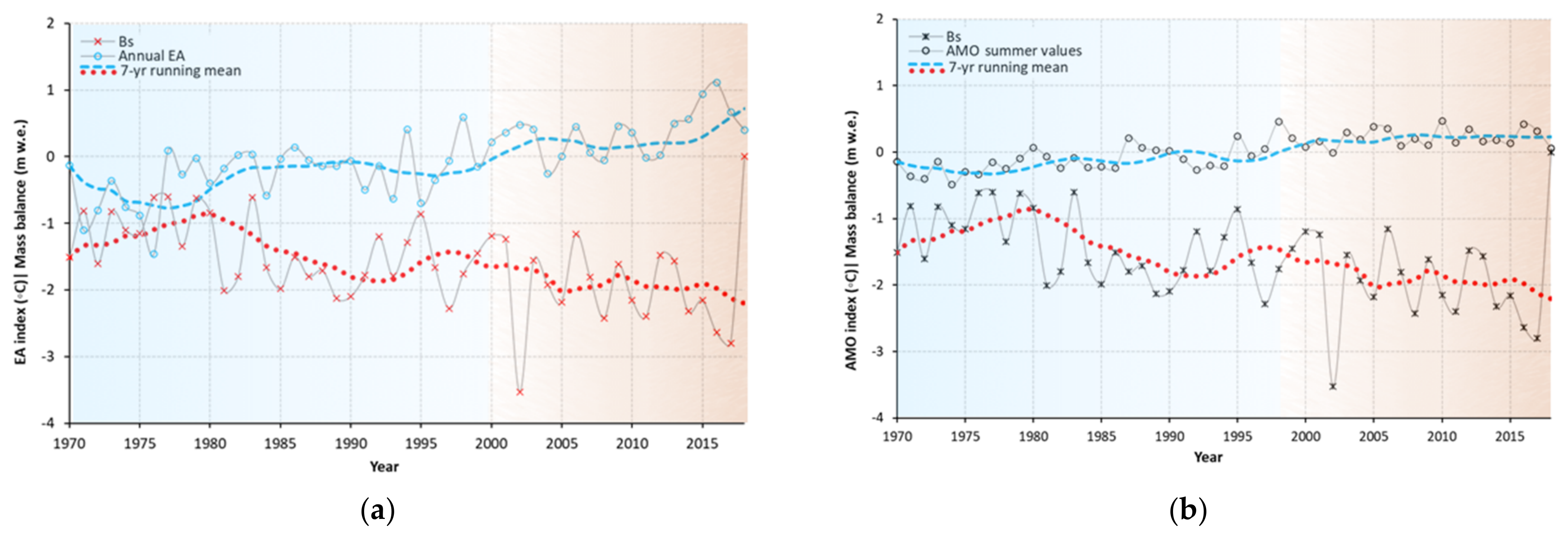
The correlation analysis indicates that there is predominantly a positive relationship between winter mass balance and seasonal and annual teleconnection patterns (Table 8). Although the corresponding values are not highly significant, there are negative correlations between winter mass balance and winter GBI and the summer NAOHurrell index. The correlations between summer balance and the selected indices are mostly significant (p < 0.05). A strong relationship is found between the annual AMO and EA indices and summer mass balance with correlation coefficients of −0.86 and −0.88 (p < 0.05), respectively. The ten lowest Bs had summer AMO and EA mean values of 0.22 and 0.46, respectively. Further, the summer GBI index is significantly anticorrelated with summer mass balance patterns in Switzerland. The summer GBI tends to direct the North Atlantic storm track and associated moisture over Northern Europe and concurrently influence a warming and drying effect over much of the central/southern continent [53]. In contrast to other indices, both summer NAOCPC and SCA show a positive correlation with summer mass balances, r = 0.69 and 0.66 (p < 0.05), respectively. However, the lagged associations between the teleconnections and summer and annual mass balance should be taken into account, as cold season precipitation (presumably snow) influences the melt rates of the following summer.
In addition to the correlation between summer and winter balances, we also examined the relationship between annual balance and teleconnection patterns. In general, seasonal and annual AMO, GBI, and EA show statistically significant, negative correlations with the annual balance of the Swiss glaciers. In comparison with the other indices, we conclude that the summer and annual balance of the Swiss glaciers are largely driven by AMO and EA behaviors (Table 8). Figure 7 highlights this strong negative association between summer mass balance and summer AMO (r =−0.86) and annual EA (r =−0.88), as well as the consistency of EA and AMO staying above 0 °C since the late 1990s. This is well corroborated by Huss’s (2010) findings, showing that the decadal AMO and mass balance of Swiss glaciers exhibit a strong and negative correlation of 0.78 [32]. Our findings similarly suggest that the positive (warmer-than-average) North Atlantic sea surface temperature (SST) anomalies amplify glacier mass losses (Figure 7), perhaps through warmer regional air temperatures and increased rain versus snow at high altitudes. In contrast, negative (cool) SST anomalies are associated with periods of cooler air temperatures and more snowfall, resulting in positive mass balance.
The oceanic surface temperature conditions are linked to the mass balance of the Swiss glaciers through atmospheric circulation. For instance, under a positive NAO regime, low pressure near Iceland and high pressure over the Azores work in tandem to promote a zonal jet stream and westerly winds that transport warm, moist air from the North Atlantic Ocean to continental Europe.
Comas-Bru and McDermott (2014) noted the association of positive NAO, EA, and SCA indices with below-normal winter precipitation and colder winters in southern Europe [90]. The authors also examined the relationship between the indices and found that winter precipitation patterns are affected by the state and combination of the NAO with either the EA or the SCA; NAO and EA patterns of the same sign coincide with poleward migration of the Icelandic Low and Azores High over North Atlantic waters. When positive phasing occurs between the patterns, the northward shifted jet stream leads to decreased precipitation over central and southern Europe. On the other hand, in-phase NAO and SCA patterns tend to coincide with low pressure atop Greenland with the subtropical high situated over Western Europe. This meridional jet stream configuration produces southwesterly flow and increased precipitation across Scotland and northern Scandinavia while drier conditions persist across much of central Europe [90].
These spatial precipitation patterns, in part modulated by the ocean–atmosphere climate modes, are supported by the strong anticorrelation found herein between the EA pattern and Swiss glaciers’ mass balance characteristics (e.g., positive EA tends to yield less precipitation to the region). Future work will further explore observed seasonal mass balance responses to teleconnection phasing and related ocean–atmosphere interactions, including patterns of temperature advection off the mid-to-high latitude North Atlantic Ocean.

5.4. Hypsometric Characteristic and Terminus Retreat

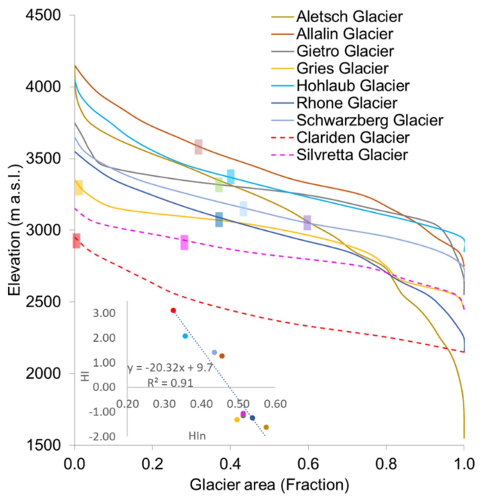
Hypsometric analyses of the studied glaciers provide some new insights (Figure 8). In general, the shape of the hypsometric curve explains the temporal changes in the slope of the original basin. Strahler classified the drainage basins as youth (convex upward curves), mature (S-shaped curves that are concave upward at high elevations and convex downward at low elevations) and peneplain or distorted (concave upward curves) [91].
In addition to describing the stages of the landscape evolution, these hypsometric curves also provide an indication of erosion status for a watershed. HIn, in general, gives an estimate of the distribution of landmass volume above a reference plane [92], and for a glacier, it may represent the geometry and corresponding volumetric distribution of ice and snow. The inset plot in Figure 8 shows a significant congruence between HI and HIn for the selected glaciers, further highlighting the agreeable inferred geometry of the glaciers represented in Table 9.
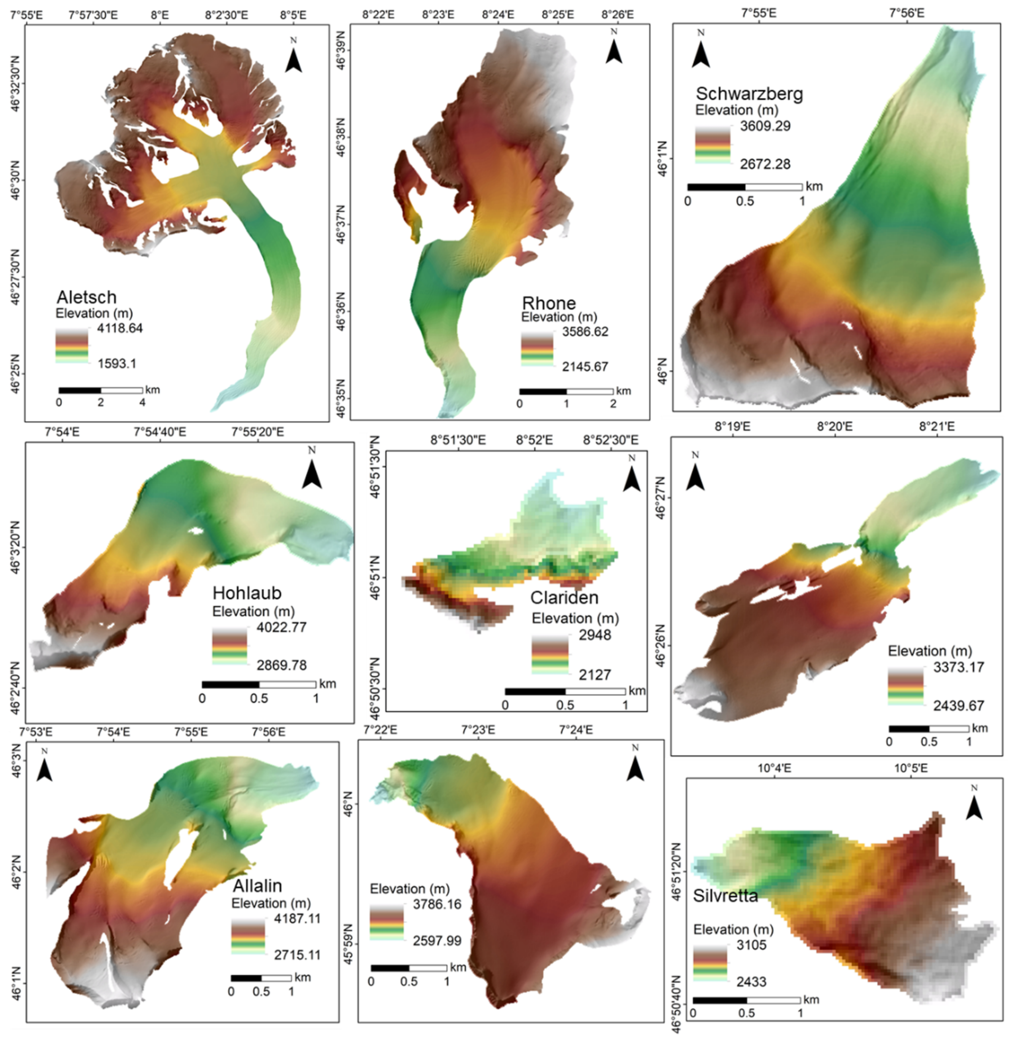
HI and corresponding shapes are compiled in Table 9. We note that the two DEMs used for this analysis are based on availability and differ in origin and source data, spatial resolutions, accuracy, and processing steps (Figure 9). As described in Section 5.1, the rate of mass balance change after the 1980s became negative for Allalin and Hohlaub. According to Table 9 and Figure 8, both glaciers are bottom-heavy with N-NE facing aspects. In Gietro and Silvretta, the rates also significantly changed from −200 to −1000 mm w.e., indicating heavy mass loss for these glaciers in near future. It is interesting to note that these two are the only equidimensional glaciers in the study area and both have N-NW aspect (Table 9 and Figure 8).
Similarly, the correlation analysis of Ba presented in Section 5.1 reveals two distinct classes. Silvretta, Gries, and Gietro can be categorized into one group as per correlations (Figure 3) and equidimensional morphologies. Allalin, Schwarzberg, and Hohlaub show a stronger correlation with each other, and interestingly, all three glaciers display bottom-heavy or very bottom-heavy morphologies. Aletsch is the only glacier with ELA below the mean elevation [26,33], and the fluctuation of this glacier near mean is well-supported by its very top-heavy morphology (Table 9). The dashed curves in Figure 8 represent the two glaciers outside the catchment, and the remarkably distinct morphologies of these two glaciers are apparent in the shape of the curves.
Silvretta, in particular, is located in a very narrow elevation range of 672 m, and its hypsometric curve is nearest to a straight line, highlighting its equidimensional shape. The three glaciers with the highest AAR (Table), i.e., Aletsch, Rhone, and Schwarzberg, have similar S-shaped curves that are distinct from the rest of the glaciers (Figure 8). A comparative analysis between Clariden and Gries reveals another interesting facet. These two glaciers are within ~2400–3300 m, have similar area, and have NE facing aspect (Table 1). Clariden displays a convex curve, making it very bottom-heavy, while Gries has a distinct concave profile for the majority of its middle elevations, thus making it an equidimensional glacier (Figure 8). During the accumulation season, Clariden on average showed the highest accumulation (1385 mm w.e.), while in the same period, the lowest average annual mass balance of −919 mm w.e. was observed for Gries. Similarly, the mean AAR was the lowest for Gries (26%) and the highest for Clariden (56%) from 1970 to 2017. The very bottom-heavy morphology of Clariden, its gentler slope than Gries (Figure 9), and significant winter accumulation are well coupled with Ba and Bw (Table 4). Thus, these observations highlight the observed correlations and mass balance trends in agreement with hypsometric distribution and morphology of glaciers. Future morphological changes due to continued mass loss in these glaciers have the potential to further accelerate the rate of negative mass balance.
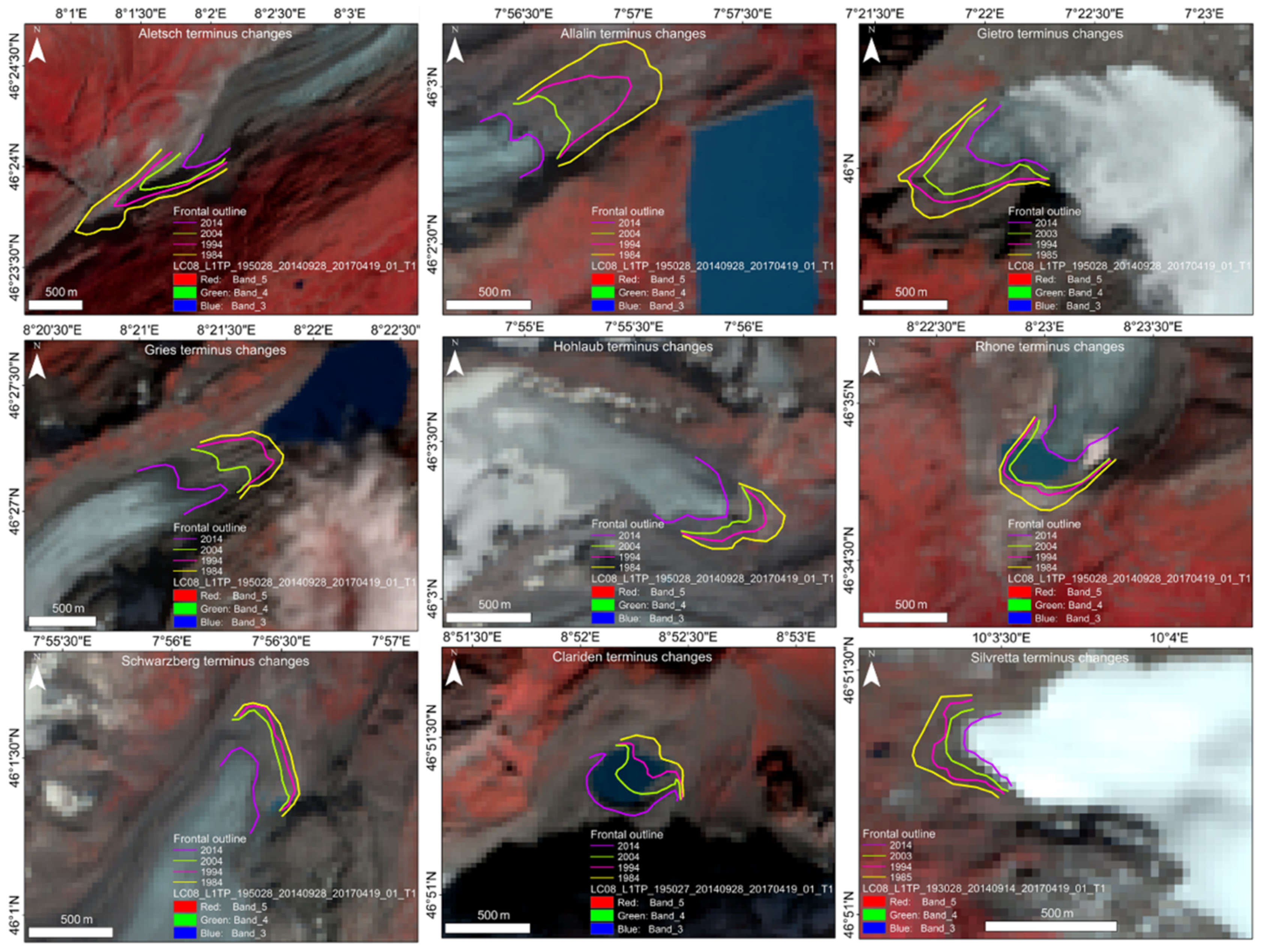
We further observed the effect of local climate controls and hypsometry on the glacier termini changes over the past three decades (1984–2014) (Figure 10 and Table 10). The frontal retreat patterns reveal a significant spatiotemporal disparity (Table 10). Apart from Allalin and Silvretta, all the glaciers show higher retreat rates in the recent decade (2004–2014). The retreat rate is even stronger for the two bottom-heavy glaciers in the Mattmark region, i.e., Hohlaub and Schwarzberg, at ~50% and ~647%, respectively, higher than the previous decade (Figure 10, Table 10). The dramatic retreat of Schwarzberg can be attributed to a substantial mass imbalance since the 1990s (μBa = −640 mm w.e., σ = 650 mm w.e., rate of change = −641 mm w.e.) that reciprocated in its extreme terminus retreat rate in the next decade. As mentioned above, the three glaciers with the highest AAR (Table 1), i.e., Aletsch, Rhone, and Schwarzberg, have smoother S-shaped curve that are distinct from the rest of the glaciers (Figure 8).
Table 10 reveals that Rhone has also followed the same substantial retreat path of Schwarzberg in the recent decade (2004–2014) with the retreat rate increasing by ~424% compared to the previous decade. It is notable that the decadal retreat of Aletsch was considerably higher (>1100 m) from 1984 to 2014 (Table 10). WGMS report also confirms the accelerated thinning of this glacier since the late 1980s [26]. Being the largest glacier in the Alps, it indicates varying climatic controls over its accumulation and ablation zones. Although the local climate of Aletsch’s front is characterized as dry, the accumulation area receives a high amount of precipitation due to regional advection effects [49].

6. Conclusions

This study effectively used the available glaciological, terrain, and remote sensing data to provide updated analyses of long-term annual and seasonal mass balance time series of glaciers across the Swiss Alps. The purpose of this analysis was to identify trends/changes in the mass balance series and study the relationship between the components of mass balance, and local climatic variables and large-scale oceanic and atmospheric patterns. The most prominent result of this research is the significant glacier mass loss and acceleration in ablation due to the warming signals influenced by North Atlantic climate patterns. According to the results emerging from this analysis, the following conclusions can be reached:
-
All selected glaciers have lost their equilibrium condition in the recent century, and persistent negative annual mass balance trends, accompanied by decreasing AARs, have been observed for the glaciers located in the south of Switzerland.
-
Such imbalanced behavior is the product of ablation induced by warmer temperatures, increased melting, and acceleration of the ice-albedo feedback process. Although the precipitation trends are not significant, the increase in the number of days with the air temperature above 0 °C supports the reduction in solid precipitation over the glaciers. Additionally, rain-on-snow events may also be another contributor to the ice mass loss in these regions.
-
The analyzed glaciers reveal that the annual mass balances are mainly controlled by the summer mass balance, which is statistically attributed to the significant anticorrelation with summer air temperature.
-
Atmosphere–ocean teleconnection patterns, including AMO and EA, are strongly linked through the time to mass balance characteristics of the southern Swiss Alps, and these large-scale climatic forcings will likely continue to influence surface mass balance regime.
-
Most of the observed glaciers are losing accumulation area given that AAR percent has dropped from approximately 75% in 1970 to 25% in recent years, which highlights the acceleration of the melt rate.
-
Although a decadal frontal retreat analysis during 1984–2014 reveals significant spatiotemporal variations, nearly all glaciers have considerably receded during 2004–2014. This highlights the possibility of continuing high melt rates in the next decades and corroborates the mass balance–climate coupling in the region.
-
Based on the current research and the corresponding results, the negative mass balance trends cannot be simply attributed to the direct response of global warming. Hence, we emphasize that future investigations should focus on resolving complex and indirect surface–atmosphere interactions (e.g., reflectivity and impurities of glacier surfaces [93]) to more comprehensively understand physical processes driving glacier mass balance variability. In particular, the hypsometric evolution of glaciers with continued mass loss warrants considering dynamic modeling approaches to simulate the future state of glaciers as we observe glacier hypsometry and morphology playing considerable roles in defining mass balance trends. In an attempt to better understand the physical drivers of the Swiss glaciers’ mass balance, we recommend that future work provide a deeper evaluation of the spatiotemporal impacts of climatic teleconnections on the glaciers, including analyzing patterns of regional temperature advection along with wind speed and direction variations as it relates to changing glacial conditions.

Author Contributions

Conceptualization, S.G., J.L.R.J., and T.J.B.; methodology, S.G., A.B., and T.J.B.; software, S.G. and L.S.; validation, S.G.; formal analysis, S.G., A.B., and L.S.; investigation, S.G.; resources, S.G. and T.J.B.; data curation, S.G.; writing—original draft preparation, S.G. and A.B.; writing—review and editing, S.G., J.L.R.J., T.J.B., D.R.B., R.C.W., and A.B.; visualization, S.G., L.S., and A.B.; supervision, J.L.R.J., T.J.B., R.C.W., and D.R.B.; funding acquisition, S.G. and J.L.R.J. All authors have read and agreed to the published version of the manuscript.

Funding

This research was funded by Texas State University through the Doctoral Research Support Fellowship. Support for T.J.B. was provided by the University of Alaska Fairbanks Experimental Arctic Prediction Initiative.

Institutional Review Board Statement

Not applicable.

Informed Consent Statement

Not applicable.

Data Availability Statement

The monthly CPC teleconnections (NAO, EA, SCA) are available at the CPC website. The NAO (Cropper daily version) can be obtained from Thomas Cropper, the NAO (Hurrell version) from Climate Data Guide, and the daily GBI [53] from NOAA. The AMO monthly data is also available at NOAA.

Acknowledgments

Weather data were purchased from MeteoSwiss and delivered by Gergely Rigo. We thank Huss for sharing annual and seasonal mass balance datasets, and Klimeš for revising the earlier manuscript draft.

Conflicts of Interest

The authors declare no conflict of interest.

Abbreviations

The following abbreviations are used in this manuscript:
AMOAtlantic Multidecadal Oscillation
AARsaccumulation area ratios
GBIGreenland Blocking Index
EAEast Atlantic pattern
WGMSworld glacier monitoring service
GTNGglobal terrestrial network for glaciers
NAOEANorth Atlantic Oscillation
GLOFsglacial lake outburst floods
ASTERadvanced spaceborne thermal emission and reflection radiometer
GDMglobal digital elevation model
SCAScandinavian pattern
VAW/ETHZlaboratory of hydraulics, hydrology, and glaciology at ETH Zürich
ELAequilibrium line altitude
Baannual mass balance
Bwwinter mass balance
Bssummer mass balance
NBCNSwiss national basic climatological network
NOAANational Oceanic and Atmospheric Administration
CPCNOAA Climatic Prediction Center
EOFempirical orthogonal function
CUSUMcumulated sum of standard residuals
efpempirical fluctuation process
BICBayesian information criterion
ACFautocorrelation
PACFpartial autocorrelation
HIhypsometric index
HInhypsometric integral
RMSEroot mean square error

References

  1. Fischer, M.; Huss, M.; Hoelzle, M. Surface elevation and mass changes of all Swiss glaciers 1980–2010. Cryosphere 2015, 9, 525–540. [Google Scholar] [CrossRef] [Green Version]
  2. Zemp, M.; Frey, H.; Gärtner-Roer, I.; Nussbaumer, S.U.; Hoelzle, M.; Paul, F.; Haeberli, W.; Denzinger, F.; Ahlstrøm, A.P.; Anderson, B.; et al. Historically unprecedented global glacier decline in the early 21st century. J. Glaciol. 2015, 61, 745–762. [Google Scholar] [CrossRef] [Green Version]
  3. Carturan, L.; Baroni, C.; Brunetti, M.; Carton, A.; Fontana, G.D.; Salvatore, M.C.; Zanoner, T.; Zuecco, G. Analysis of the mass balance time series of glaciers in the Italian Alps. Cryosphere 2016, 10, 695–712. [Google Scholar] [CrossRef] [Green Version]
  4. Medwedeff, W.G.; Roe, G.H. Trends and variability in the global dataset of glacier mass balance. Clim. Dyn. 2016, 48, 3085–3097. [Google Scholar] [CrossRef]
  5. Naegeli, K.; Huss, M. Sensitivity of mountain glacier mass balance to changes in bare-ice albedo. Ann. Glaciol. 2017, 58, 119–129. [Google Scholar] [CrossRef] [Green Version]
  6. Huss, M.; Bauder, A. 20th-century climate change inferred from four long-term point observations of seasonal mass balance. Ann. Glaciol. 2009, 50, 207–214. [Google Scholar] [CrossRef] [Green Version]
  7. Miller, J.D.; Immerzeel, W.W.; Rees, G. Climate Change Impacts on Glacier Hydrology and River Discharge in the Hindu Kush–Himalayas: A Synthesis of the Scientific Basis. Mt. Res. Dev. 2012, 32, 461–467. [Google Scholar]
  8. Schleiss, A.; Oberrauch, F. Flexibilisierung Der Wasserkraft in Der Schweiz Für Zukünftige Aufgaben Im Internationalen Strommarkt. Wasser Energ. Luft 2014, 106, 175–178. [Google Scholar]
  9. Piot, M. Wirtschaftlichkeit der Wasserkraft in der Schweiz. Wasserwirtschaft 2017, 107, 33–38. [Google Scholar] [CrossRef]
  10. Rahman, K.; da Silva, A.G.; Tejeda, E.M.; Gobiet, A.; Beniston, M.; Lehmann, A. An independent and combined effect analysis of land use and climate change in the upper Rhone River watershed, Switzerland. Appl. Geogr. 2015, 63, 264–272. [Google Scholar] [CrossRef]
  11. Rasul, G.; Molden, D. The Global Social and Economic Consequences of Mountain Cryospheric Change. Front. Environ. Sci. 2019, 7, 91. [Google Scholar] [CrossRef]
  12. Milner, A.M.; Khamis, K.; Battin, T.J.; Brittain, J.E.; Barrand, N.E.; Füreder, L.; Cauvy-Fraunié, S.; Gíslason, G.M.; Jacobsen, D.; Hannah, D.M.; et al. Glacier shrinkage driving global changes in downstream systems. Proc. Natl. Acad. Sci. USA 2017, 114, 9770–9778. [Google Scholar] [CrossRef] [Green Version]
  13. Immerzeel, W.W.; Van Beek, L.P.H.; Bierkens, M.F.P. Climate change will affect the Asian Water Towers. Science 2010, 328, 1382–1385. [Google Scholar]
  14. Chevallier, P.; Pouyaud, B.; Suarez, W.; Condom, T. Climate change threats to environment in the tropical Andes: Glaciers and water resources. Reg. Environ. Chang. 2011, 11, 179–187. [Google Scholar] [CrossRef]
  15. Huggel, C.; Haeberli, W.; Kääb, A.; Bieri, D.; Richardson, S. An assessment procedure for glacial hazards in the Swiss Alps. Can. Geotech. J. 2004, 41, 1068–1083. [Google Scholar] [CrossRef]
  16. Klimeš, J.; Novotný, J.; Novotná, I.; De Urries, B.J.; Vilímek, V.; Emmer, A.; Strozzi, T.; Kusák, M.; Rapre, A.C.; Hartvich, F.; et al. Landslides in moraines as triggers of glacial lake outburst floods: Example from Palcacocha Lake (Cordillera Blanca, Peru). Landslides 2016, 13, 1461–1477. [Google Scholar] [CrossRef]
  17. Haeberli, W.; Buetler, M.; Huggel, C.; Friedli, T.L.; Schaub, Y.; Schleiss, A.J. New lakes in deglaciating high-mountain regions–opportunities and risks. Clim. Chang. 2016, 139, 201–214. [Google Scholar] [CrossRef]
  18. Harrison, S.; Kargel, J.S.; Huggel, C.; Reynolds, J.; Shugar, D.H.; Betts, R.A.; Emmer, A.; Glasser, N.; Haritashya, U.K.; Klimeš, J.; et al. Climate change and the global pattern of moraine-dammed glacial lake outburst floods. Cryosphere 2018, 12, 1195–1209. [Google Scholar] [CrossRef] [Green Version]
  19. Koenig, U.; Abegg, B. Impacts of Climate Change on Winter Tourism in the Swiss Alps. J. Sustain. Tour. 1997, 5, 46–58. [Google Scholar] [CrossRef]
  20. Spandre, P.; François, H.; Verfaillie, D.; Pons, M.; Vernay, M.; Lafaysse, M.; George, E.; Morin, S. Winter tourism under climate change in the Pyrenees and the French Alps: Relevance of snowmaking as a technical adaptation. Cryosphere 2019, 13, 1325–1347. [Google Scholar] [CrossRef] [Green Version]
  21. Spandre, P.; François, H.; Verfaillie, D.; Lafaysse, M.; Déqué, M.; Eckert, N.; George, E.; Morin, S. Climate controls on snow reliability in French Alps ski resorts. Sci. Rep. 2019, 9, 1–9. [Google Scholar] [CrossRef] [Green Version]
  22. Demiroglu, O.C.; Dannevig, H.; Aall, C. Climate change acknowledgement and responses of summer (glacier) ski visitors in Norway. Scand. J. Hosp. Tour. 2018, 18, 419–438. [Google Scholar] [CrossRef] [Green Version]
  23. Braithwaite, R.J. Glacier mass balance: The first 50 years of international monitoring. Prog. Phys. Geogr. Earth Environ. 2002, 26, 76–95. [Google Scholar] [CrossRef]
  24. Hall, M. II.—Les Variations Périodiques Des Glaciers. Discours Préliminaire. Par F. A. Forel, President de La Commission Internationale Des Glaciers. Archives Des Sciences Physiques et Naturelles. Genève. Vol. Xxxiv, p. 209. Geol. Mag. 1895, 2, 569–570. [Google Scholar]
  25. Haeberli, W.; Hoelzle, M.; Suter, S.; World Glacier Monitoring Service. Studies and reports in hydrology. In Into the Second Century of Worldwide Glacier Monitoring-Prospects and Strategies: A Contribution to the International Hydrological Programme (IHP) and the Global Environment Monitoring System (GEMS); UNESCO: Paris, France, 1998. [Google Scholar]
  26. World Glacier Monitoring Service (WGMS). Fluctuations of Glaciers Database; WGMS: Zurich, Switzerland, 2017. [Google Scholar]
  27. Holzhauser, H. Die bewegte Vergangenheit des Grossen Aletschgletschers. Bl. Aus Walliser Gesch. 2009, 47. [Google Scholar]
  28. Abermann, J.; Lambrecht, A.; Fischer, A.; Kuhn, M. Quantifying changes and trends in glacier area and volume in the Austrian Ötztal Alps (1969–1997–2006). Cryosphere 2009, 3, 205–215. [Google Scholar] [CrossRef] [Green Version]
  29. Carturan, L.; Filippi, R.; Seppi, R.; Gabrielli, P.; Notarnicola, C.; Bertoldi, L.; Paul, F.; Rastner, P.; Cazorzi, F.; Dinale, R.; et al. Area and volume loss of the glaciers in the Ortles-Cevedale group (Eastern Italian Alps): Controls and imbalance of the remaining glaciers. Cryosphere 2013, 7, 1339–1359. [Google Scholar] [CrossRef] [Green Version]
  30. Zemp, M.; Paul, F.; Hoelzle, M.; Haeberli, W. Glacier fluctuations in the European Alps, 1850–2000: An overview and spatio-temporal analysis of available data. In Darkening Peaks: Glacier Retreat, Science, and Society; Orlove, B., Wiegandt, E., Luckman, B.H., Eds.; University of California Press: Berkeley, CA, USA, 2008; pp. 152–167. [Google Scholar]
  31. Huss, M.; Usselmann, S.; Farinotti, D.; Bauder, A. Glacier mass balance in the south-eastern Swiss Alps since 1900 and perspectives for the future. Erdkunde 2010, 2010, 119–140. [Google Scholar] [CrossRef] [Green Version]
  32. Huss, M.; Hock, R.; Bauder, A.; Funk, M. 100-year mass changes in the Swiss Alps linked to the Atlantic Multidecadal Oscillation. Geophys. Res. Lett. 2010, 37, 10. [Google Scholar] [CrossRef] [Green Version]
  33. Huss, M.; Dhulst, L.; Bauder, A. New long-term mass-balance series for the Swiss Alps. J. Glaciol. 2015, 61, 551–562. [Google Scholar] [CrossRef] [Green Version]
  34. Oerlemans, J.; Anderson, B.; Hubbard, A.; Huybrechts, P.; Jóhannesson, T.; Knap, W.H.; Schmeits, M.; Stroeven, A.P.; Van De Wal, R.S.W.; Wallinga, J.; et al. Modelling the response of glaciers to climate warming. Clim. Dyn. 1998, 14, 267–274. [Google Scholar] [CrossRef] [Green Version]
  35. Braithwaite, R.J.; Zhang, Y. Sensitivity of mass balance of five Swiss glaciers to temperature changes assessed by tuning a degree-day model. J. Glaciol. 2000, 46, 7–14. [Google Scholar] [CrossRef] [Green Version]
  36. Oerlemans, J.; Reichert, B.K. Relating glacier mass balance to meteorological data by using a seasonal sensitivity characteristic. J. Glaciol. 2000, 46, 1–6. [Google Scholar] [CrossRef] [Green Version]
  37. (Lisette) Klok, E.; Oerlemans, J. Model study of the spatial distribution of the energy and mass balance of Morteratschgletscher, Switzerland. J. Glaciol. 2002, 48, 505–518. [Google Scholar] [CrossRef] [Green Version]
  38. Woul, M.D.; Hock, R. Static Mass-Balance Sensitivity of Arctic Glaciers and Ice Caps Using a Degree-Day Approach. Ann. Glaciol. 2005, 42, 217–224. [Google Scholar] [CrossRef] [Green Version]
  39. Zhu, M.; Yao, T.; Yang, W.; Xu, B.; Wu, G.; Wang, X. Differences in Mass Balance Behavior for Three Glaciers from Different Climatic Regions on the Tibetan Plateau. Clim. Dyn. 2018, 50, 3457–3484. [Google Scholar] [CrossRef]
  40. Huss, M.; Fischer, M. Sensitivity of Very Small Glaciers in the Swiss Alps to Future Climate Change. Front. Earth Sci. 2016, 4, 4. [Google Scholar] [CrossRef] [Green Version]
  41. McCabe, G.J.; Fountain, A.G.; Dyurgerov, M. Variability in Winter Mass Balance of Northern Hemisphere Glaciers and Relations with Atmospheric Circulation. Arct. Antarct. Alp. Res. 2000, 32, 64–72. [Google Scholar] [CrossRef]
  42. Shahgedanova, M.; Stokes, C.R.; Gurney, S.D.; Popovnin, V. Interactions between mass balance, atmospheric circulation, and recent climate change on the Djankuat Glacier, Caucasus Mountains, Russia. J. Geophys. Res. Space Phys. 2005, 110, 04108. [Google Scholar] [CrossRef]
  43. Marzeion, B.; Nesje, A. Spatial patterns of North Atlantic Oscillation influence on mass balance variability of European glaciers. Cryosphere 2012, 6, 661–673. [Google Scholar] [CrossRef] [Green Version]
  44. Thibert, E.; Eckert, N.; Vincent, C. Climatic Drivers of Seasonal Glacier Mass Balances: An Analysis of 6 Decades at Glacier de Sarennes (French Alps). Cryosphere 2013, 7, 47–66. [Google Scholar]
  45. Beniston, M. Variations of snow depth and duration in the swiss alps over the last 50 years: Links to changes in large-scale climatic forcings. Clim. Chang. 1997, 36, 281–300. [Google Scholar] [CrossRef]
  46. Gharehchahi, S.; James, W.H.M.; Bhardwaj, A.; Jensen, J.L.R.; Sam, L.; Ballinger, T.J.; Butler, D.R. Glacier Ice Thickness Estimation and Future Lake Formation in Swiss Southwestern Alps—The Upper Rhône Catchment: A VOLTA Application. Remote Sens. 2020, 12, 3443. [Google Scholar]
  47. Vihma, T.; Graversen, R.; Chen, L.; Handorf, D.; Skific, N.; Francis, J.A.; Tyrrell, N.; Hall, R.; Hanna, E.; Uotila, P.; et al. Effects of the Tropospheric Large-scale Circulation on European Winter Temperatures during the Period of Amplified Arctic Warming. Int. J. Climatol. 2020, 40, 509–529. [Google Scholar] [PubMed] [Green Version]
  48. Kropáček, J.; Neckel, N.; Bauder, A. Estimation of Mass Balance of the Grosser Aletschgletscher, Swiss Alps, from ICESat Laser Altimetry Data and Digital Elevation Models. Remote Sens. 2014, 6, 5614–5632. [Google Scholar] [CrossRef] [Green Version]
  49. Schwarb, M.; Schär, C.J. The Alpine Precipitation Climate. In Evaluation of a High-Resolution Analysis Scheme Using Comprehensive Rain-Gauge Data; ETH Zürich: Zürich, Switzerland, 2000. [Google Scholar]
  50. Spatial Climate Analyses-MeteoSwiss. Available online: https://www.meteoswiss.admin.ch/home/climate/swiss-climate-in-detail/raeumliche-klimaanalysen.html (accessed on 22 October 2019).
  51. Fang, Z.-F. Statistical Relationship Between the Northern Hemisphere Sea Ice and Atmospheric Circulation During Wintertime. In Observation, Theory and Modeling of Atmospheric Variability; World Scientific Series on Asia-Pacific Weather and Climate; World Scientific: Singapore, 2004; Volume 3, pp. 131–141. [Google Scholar]
  52. Hanna, E.; Fettweis, X.; Mernild, S.H.; Cappelen, J.; Ribergaard, M.H.; Shuman, C.A.; Steffen, K.; Wood, L.; Mote, T.L. Atmospheric and oceanic climate forcing of the exceptional Greenland ice sheet surface melt in summer 2012. Int. J. Clim. 2013, 34, 1022–1037. [Google Scholar] [CrossRef] [Green Version]
  53. Hanna, E.; Cropper, T.E.; Hall, R.J.; Cappelen, J. Greenland Blocking Index 1851–2015: A regional climate change signal. Int. J. Clim. 2016, 36, 4847–4861. [Google Scholar] [CrossRef] [Green Version]
  54. Hanna, E.; Hall, R.J.; Cropper, T.E.; Ballinger, T.J.; Wake, L.; Mote, T.; Cappelen, J. Greenland Blocking Index Daily Series 1851–2015: Analysis of Changes in Extremes and Links with North Atlantic and UK Climate Variability and Change. Int. J. Climatol. 2018, 38, 3546–3564. [Google Scholar]
  55. Hurrell, J.W. Decadal Trends in the North Atlantic Oscillation: Regional Temperatures and Precipitation. Science 1995, 269, 676–679. [Google Scholar] [CrossRef] [Green Version]
  56. Wallace, J.M.; Gutzler, D.S. Teleconnections in the Geopotential Height Field during the Northern Hemisphere Winter. Mon. Weather Rev. 1981, 109, 784–812. [Google Scholar]
  57. Barnston, A.G.; Livezey, R.E. Classification, Seasonality and Persistence of Low-Frequency Atmospheric Circulation Patterns. Mon. Weather Rev. 1987, 115, 1083–1126. [Google Scholar]
  58. Kaplan, A.; Cane, M.A.; Kushnir, Y.; Clement, A.C.; Blumenthal, M.B.; Rajagopalan, B. Analyses of global sea surface temperature 1856–1991. J. Geophys. Res. Space Phys. 1998, 103, 18567–18589. [Google Scholar] [CrossRef] [Green Version]
  59. Enfield, D.B.; Mestas-Nuñez, A.M.; Trimble, P.J. The Atlantic Multidecadal Oscillation and its relation to rainfall and river flows in the continental U.S. Geophys. Res. Lett. 2001, 28, 2077–2080. [Google Scholar] [CrossRef] [Green Version]
  60. Knight, J.R.; Folland, C.K.; Scaife, A.A. Climate impacts of the Atlantic Multidecadal Oscillation. Geophys. Res. Lett. 2006, 33, 17706. [Google Scholar] [CrossRef] [Green Version]
  61. Federal Office of Topography, Swisstopo Online Shop. Available online: https://shop.swisstopo.admin-.ch/en/products/height_models/alti3D (accessed on 7 October 2019).
  62. LP DAAC-NASA and METI Release ASTER Global DEM Version 3. Available online: https://lpdaac.usgs.gov/news/nasa-and-meti-release-aster-global-dem-version-3/ (accessed on 21 November 2019).
  63. USGS. Earth Explorer. Available online: https://earthexplorer.usgs.gov/ (accessed on 28 August 2016).
  64. Beniston, M. Mountain Climates and Climatic Change: An Overview of Processes Focusing on the European Alps. Pure Appl. Geophys. 2005, 162, 1587–1606. [Google Scholar] [CrossRef] [Green Version]
  65. Scherrer, S.; Appenzeller, C. Swiss Alpine snow pack variability: Major patterns and links to local climate and large-scale flow. Clim. Res. 2006, 32, 187–199. [Google Scholar] [CrossRef] [Green Version]
  66. Zeileis, A.; Kleiber, C.; Krämer, W.; Hornik, K. Testing and dating of structural changes in practice. Comput. Stat. Data Anal. 2003, 44, 109–123. [Google Scholar] [CrossRef] [Green Version]
  67. Bai, J. Estimation of a Change Point in Multiple Regression Models. Rev. Econ. Stat. 1997, 79, 551–563. [Google Scholar] [CrossRef]
  68. Hawkins, D.M. Fitting multiple change-point models to data. Comput. Stat. Data Anal. 2001, 37, 323–341. [Google Scholar] [CrossRef]
  69. Sullivan, J.H. Estimating the Locations of Multiple Change Points in the Mean. Comput. Stat. 2002, 17, 289–296. [Google Scholar] [CrossRef]
  70. Bai, J.; Perron, P. Computation and analysis of multiple structural change models. J. Appl. Econ. 2002, 18, 1–22. [Google Scholar] [CrossRef] [Green Version]
  71. Zeileis, A. Alternative boundaries for CUSUM tests. Stat. Pap. 2004, 45, 123–131. [Google Scholar] [CrossRef]
  72. Andrews, D.W.K.; Ploberger, W. Optimal Tests when a Nuisance Parameter is Present Only Under the Alternative. Econometrica 1994, 62, 1383. [Google Scholar] [CrossRef]
  73. Kuan, C.-M.; Hornik, K. The generalized fluctuation test: A unifying view. Econ. Rev. 1995, 14, 135–161. [Google Scholar] [CrossRef]
  74. Brown, R.L.; Durbin, J.; Evans, J.M. Techniques for Testing the Constancy of Regression Relationships Over Time. J. R. Stat. Soc. Ser. B (Methodol.) 1975, 37, 149–163. [Google Scholar] [CrossRef]
  75. Ploberger, W.; Krämer, W. The Cusum Test with Ols Residuals. Econometrica 1992, 60, 271. [Google Scholar] [CrossRef]
  76. Kleiber, C.; Zeileis, A. Applied Econometrics with R; Springer: New York, NY, USA, 2008. [Google Scholar]
  77. Chow, G.C. Tests of Equality Between Sets of Coefficients in Two Linear Regressions. Econometrica 1960, 28, 591. [Google Scholar] [CrossRef]
  78. Helsel, D.R.; Hirsch, R.M. Applicability of the t-Test for Detecting Trends in Water Quality Variables, by Robert H. Montgomery and Jim C. Loftis. JAWRA J. Am. Water Resour. Assoc. 1988, 24, 201–204. [Google Scholar] [CrossRef]
  79. Mann, H.B. Nonparametric tests against trend. Econometrica 1945, 13, 245–259. [Google Scholar] [CrossRef]
  80. Stuart, A. Rank Correlation Methods. By M. G. Kendall, 2nd Edition. Br. J. Stat. Psychol. 1956, 9, 68. [Google Scholar]
  81. Jiskoot, H.; Curran, C.J.; Tessler, D.L.; Shenton, L.R. Changes in Clemenceau Icefield and Chaba Group glaciers, Canada, related to hypsometry, tributary detachment, length–slope and area–aspect relations. Ann. Glaciol. 2009, 50, 133–143. [Google Scholar] [CrossRef] [Green Version]
  82. Pike, R.J.; Wilson, S.E. Elevation-Relief Ratio, Hypsometric Integral, and Geomorphic Area-Altitude Analysis. GSA Bull. 1971, 82, 1079. [Google Scholar] [CrossRef]
  83. Li, Y.; Li, Y. Topographic and Geometric Controls on Glacier Changes in the Central Tien Shan, China, since the Little Ice Age. Ann. Glaciol. 2014, 55, 177–186. [Google Scholar] [CrossRef] [Green Version]
  84. Sam, L.; Bhardwaj, A.; Kumar, R.; Buchroithner, M.F.; Martín-Torres, F.J. Heterogeneity in topographic control on velocities of Western Himalayan glaciers. Sci. Rep. 2018, 8, 1–16. [Google Scholar] [CrossRef] [Green Version]
  85. Bjørk, A.A.; Kjær, K.H.; Korsgaard, N.J.; Khan, S.A.; Kjeldsen, K.K.; Andresen, C.S.; Box, J.E.; Larsen, N.K.; Funder, S. An aerial view of 80 years of climate-related glacier fluctuations in southeast Greenland. Nat. Geosci. 2012, 5, 427–432. [Google Scholar] [CrossRef] [Green Version]
  86. Hall, D.K.; Bayr, K.J.; Schöner, W.; Bindschadler, R.A.; Chien, J.Y. Consideration of the errors inherent in mapping historical glacier positions in Austria from the ground and space (1893–2001). Remote. Sens. Environ. 2003, 86, 566–577. [Google Scholar] [CrossRef]
  87. Thibert, E.; Sielenou, P.D.; Vionnet, V.; Eckert, N.; Vincent, C. Causes of Glacier Melt Extremes in the Alps Since 1949. Geophys. Res. Lett. 2018, 45, 817–825. [Google Scholar] [CrossRef] [Green Version]
  88. Rottler, E.; Kormann, C.; Francke, T.; Bronstert, A. Elevation-dependent warming in the Swiss Alps 1981–2017: Features, forcings and feedbacks. Int. J. Clim. 2019, 39, 2556–2568. [Google Scholar] [CrossRef]
  89. Vincent, C. Influence of climate change over the 20th Century on four French glacier mass balances. J. Geophys. Res. Space Phys. 2002, 107, ACL-4. [Google Scholar] [CrossRef]
  90. Comas-Bru, L.; McDermott, F. Impacts of the EA and SCA patterns on the European twentieth century NAO-winter climate relationship. Q. J. R. Meteorol. Soc. 2014, 140, 354–363. [Google Scholar] [CrossRef]
  91. Strahler, A.N. Hypsometric (Area-Altitude) Analysis of Erosional Topography. Geol. Soc. Am. Bull. 1952, 63, 1117. [Google Scholar] [CrossRef]
  92. Lifton, N.A.; Chase, C.G. Tectonic, Climatic and Lithologic Influences on Landscape Fractal Dimension and Hypsome-try: Implications for Landscape Evolution in the San Gabriel Mountains, California. Geomorphology 1992, 5, 77–114. [Google Scholar] [CrossRef]
  93. Naegeli, K.; Huss, M.; Hoelzle, M. Change detection of bare-ice albedo in the Swiss Alps. Cryosphere 2019, 13, 397–412. [Google Scholar] [CrossRef] [Green Version]
Figure 1. Overview maps of the research study area and the glaciers with mass balance measurements analyzed in this work (source: ESRI, USGS, NOAA, and DHM25/200). The map represents: (a) Silvretta (b) Clariden (c) Rhone (d) Gries (e) Grosser Altesch (f) Hohlaub, Allalin, Schwarzberg (g) Gietro.
Remotesensing 13 01949 g001
Figure 2. Data coverage of annual mass balances (Ba) (a) and the time series of annual mass balance (Ba), summer mass balance (Bs), winter mass balance (Bw), and accumulation area ratios (AAR) for the selected glaciers from 1914 to 2017 (b) (Source: [33]).
Remotesensing 13 01949 g002
Figure 3. A heatmap representation of the Spearman correlation matrix of detrended Ba and dendrogram of similar groups of glaciers (group 1: Silvretta (Silv.), Clariden (Clar.), Gries (Gri.) and Gietro (Gie.); group 2: Allalin (Alla.), Schwarzberg (Sch.) and Hohlaub (Hoh.)). The right bar shows the color code of the correlation coefficients (all significant at p < 0.01).
Remotesensing 13 01949 g003
Figure 4. Number of days with the temperature above 0 °C over all glaciers per year. The blue and red shades show the dominant pattern of cold and warm periods below and above 130 days, respectively.
Remotesensing 13 01949 g004
Figure 5. Winter air temperature anomalies are shown for (a) the southern Rhone (including Gietro, Hohlaub, Allalin, and Schwarzberg glaciers), (c) the northern Rhone (including Grosser Altesch, Gries, and Rhone glaciers), (e) Silvretta, (g) Clariden. Summer air temperature anomalies are presented in (b) the southern Rhone, (d) the northern Rhone, (f) Silvretta, (h) Clariden. The blue and red shades show significant changes.
Remotesensing 13 01949 g005
Figure 6. Winter total precipitation anomalies in (a) the southern Rhone, (c) the northern Rhone, (e) Silvretta, (g) Clariden. May–Sept (summer) total precipitation anomalies in (b) the southern Rhone, (d) the northern Rhone, (f) Silvretta, (h) Clariden. The blue and red shades show significant changes.
Remotesensing 13 01949 g006
Figure 7. The relationship between the annual East Atlantic (EA) (a) and summer Multidecadal Atlantic Ocean (AMO) (b) indices versus summer mass balance from 1970 to 2017, with strong negative correlation coefficients of −0.86 and −0.88 (p < 0.05), respectively, for the 38-year record.
Remotesensing 13 01949 g007
Figure 8. Comparable hypsometric profiles for selected glaciers. The colored boxes for each profile mark the ELA of the respective glacier. The dashed curves represent the two glaciers outside the catchment. The inset plot represents the relationship between HI and HIn for the studied glaciers.
Remotesensing 13 01949 g008
Figure 9. The elevation maps of the selected Swiss glaciers (Sources: swissALTI3D, and ASTER GDEM V3 for Clariden and Silvretta).
Remotesensing 13 01949 g009
Figure 10. Glacier terminus changes during 1984–2014.
Remotesensing 13 01949 g010
Table 1. Characteristics of the selected Swiss glaciers referring to the end of the observation period. Glaciers are ordered based on the time series length (Δt), elevation range (elev. range), equilibrium line altitude (ELA), area, accumulation area ratio (AAR), and the prevailing aspect. Rhone and Aletsch are the two discontinuous time series, indicating seasonal data are not available for the entire period (Source: [33]).
GlacierLocation (Alps)PeriodΔt (yr)Elev. Range (m a.s.l.)ELA (m a.s.l.)Area (km2)AAR (%)Prevailing Aspect
AllalinValais1956–2017622693–418035759.6427NE
HohlaubValais1956–2017622843–403033652.12830E
SchwarzbergValais1956–2017622680–356631555.1033NE
GriesValais1962–2017562432–330732854.340NE
GietroValais1966–2017522751–381733155.2022NW
RhoneBernese1885–2017391775–3620308515.1035S
AletschBernese1940–1999591560–4085305583.0256SE
Silvretta *Central1918–2017992474–307130252.601W
Clariden *Glarus1914–20171032534–325129354.5025NE
(* two glaciers outside the study area).
Table 2. Overview of Landsat data used for termini delineation.
YearDate of CaptureLandsat Product IDSensorGlaciers Covered
1984, 19852 September 1984LT05_L1TP_194028_19840902_20170220_01_T1Landsat 5 Thematic Mapper (TM)Aletsch, Allalin, Clariden, Gries, Hohlaub, Rhone, Schwarzberg
2 September 1984LT05_L1TP_194027_19840902_20170220_01_T1Landsat 5 TMSilvretta
12 September 1985LT05_L1TP_195028_19850912_20171212_01_T1Landsat 5 TMGietro
19944 August 1994LT05_L1TP_195027_19940804_20180215_01_T1Landsat 5 TMClariden
4 August 1994LT05_L1TP_195028_19940804_20180215_01_T1Landsat 5 TMAletsch, Allalin, Gietro, Gries, Hohlaub, Rhone, Schwarzberg
6 August 1994LT05_L1TP_193028_19940806_20180214_01_T1Landsat 5 TMSilvretta
2003, 200414 September 2003LT05_L1TP_195028_20030914_20161204_01_T1Landsat 5 TMGietro
2 September 2004LT05_L1TP_193028_20040902_20161129_01_T1Landsat 5 TMSilvretta
9 September 2004LT05_L1TP_194028_20040909_20161130_01_T1Landsat 5 TMAletsch, Allalin, Clariden, Gries, Hohlaub, Rhone, Schwarzberg
201414 September 2014LC08_L1TP_193028_20140914_20170419_01_T1Landsat 8 Operational Land Imager (OLI)Silvretta
28 September 2014LC08_L1TP_195027_20140928_20170419_01_T1 Clariden
28 September 2014LC08_L1TP_195028_20140928_20170419_01_T1Landsat 8 OLIAletsch, Allalin, Gietro, Gries, Hohlaub, Rhone, Schwarzberg
Table 3. Structural break points of Ba and the pre/post-break change coefficients (mm w.e.).
GlacierBreaksChow TestRate of Change (Seg1)Rate of Change (Seg2)Rate of Change (Seg3)
Allalin19800.01242.8−505.4-
Hohlaub19830.02140.03−647.3-
Schwarzberg1971, 19800.40, 0.00−80.2686−641.2
Gries1980, 20010.04, 0.30−91.6890−1561.4
Gietro20010.20−224.5−874.8-
Silvretta20010.00−253−1076.6-
Clariden19880.0117.3−605.5-
Table 4. Correlation coefficients of Ba versus Bw and Bs. Values in bold are significant at p < 0.01.
GlacierΔtBwBs
Allalin620.420.90
Hohlaub620.480.89
Schwarzberg620.330.89
Gries560.120.88
Gietro520.150.85
Rhone390.440.90
Aletsch590.390.92
Silvretta990.300.87
Clariden1030.460.88
Table 5. Correlation coefficients of summer, winter, and annual precipitation versus Ba. Superscripts a–c indicate significance at p < 0.01, 0.05, and 0.10, respectively.
AllalinGietroGriesHohlaubSchwarzbergSilvrettaClariden
Winter0.150.150.28 c0.050.110.220.27 b
Summer0.01−0.20−0.16−0.07−0.140.37 b0.43 a
Annual0.160.010.13−0.03−0.010.000.00
Table 6. Correlation coefficients of summer, winter, and annual air temperature versus Ba. Superscripts a–c indicate significance at p < 0.01, 0.05, and 0.10, respectively.
AllalinGietroGriesHohlaubSchwarzbergSilvrettaClariden
Winter−0.16−0.190.43 a−0.180.29 b0.32 a0.35 b
Summer−0.20−0.230.40 a−0.220.33 b−0.21−0.06
Annual0.25 c0.25 c0.51 a0.27 c0.40 a0.36 a0.27 c
Table 7. Multiple regression coefficients for winter precipitation and summer temperature explaining Ba variation of Swiss glaciers. Superscripts a–c indicate significance at p < 0.01, 0.05, and 0.10, respectively.
AllalinGietroGriesHohlaubSchwarzbergSilvrettaClariden
Winter precipitation96.69130.90116.8062.70102.34131.95167.76
Summer temperature174.30 b−123.60325.32 a231.50 c317.78 a−175.38−58.68
Intercept−318.00−648.60−409.60−89.46567.42−500.80−776.65
% of explained variability10.006.0023.009.0019.009.005.00
Table 8. Spearman correlation coefficients of Bw, Bs, and Ba versus seasonal and annual indices. Superscripts a–b specify the significance level of correlations at p < 0.05 and p < 0.10, respectively.
IndexBwBsBa
WinterSummerAnnualWinterSummerAnnualWinterSummerAnnual
AMO−0.080.01−0.050.80 a0.86 a0.86 a0.79 a0.82 a0.85 a
NAOCPC0.30 a−0.160.26 b0.41 a0.69 a0.060.26 b0.61 a0.17
NAOHurrell0.35 a0.25 b0.30 a−0.150.39 a−0.04−0.020.31 a0.06
GBI0.34 a0.13−0.150.33 a0.68 a0.51 a0.44 a0.61 a0.55 a
SCA−0.03−0.21−0.170.33 a0.66 a0.56 a0.25 b0.59 a0.47 a
EA0.140.030.070.86 a0.82 a0.88 a0.79 a0.77 a0.81 a
Table 9. HIn, HI and glacier categories.
GlaciersHInHIGlacier Geometry
Aletsch0.58−1.62very top-heavy
Allalin0.461.26bottom-heavy
Gietro0.51−1.16equidimensional
Gries0.50−1.19equidimensional
Hohlaub0.362.06very bottom-heavy
Rhone0.54−1.24top-heavy
Schwarzberg0.441.41bottom-heavy
Clariden0.323.11very bottom-heavy
Silvretta0.51−1.06equidimensional
Table 10. Glacier retreat rates during 1984–2014.
GlacierPeriodTotal Retreat (m)Retreat Rate (m/yr)
Aletsch1984–1994433.0943.31
1994–2004282.1128.21
2004–2014451.0345.10
Allalin1984–1994190.9719.10
1994–2004461.7046.17
2004–2014190.0619.01
Gietro1985–1994102.5911.40
1994–200378.088.67
2003–2014287.8126.16
Gries1984–199485.068.51
1994–2004209.2220.92
2004–2014228.6022.86
Hohlaub1984–199494.189.42
1994–200490.589.06
2004–2014136.1513.61
Rhone1984–199498.819.88
1994–200438.563.86
2004–2014202.1720.22
Schwarzberg1984–199415.431.54
1994–200430.863.09
2004–2014230.6723.07
Clariden1984–1994137.2513.72
1994–2004170.6617.07
2004–2014193.0219.30
Silvretta1984–199480.248.02
1994–200461.116.11
2004–201465.786.58
Publisher’s Note: MDPI stays neutral with regard to jurisdictional claims in published maps and institutional affiliations.