Accelerating Haze Removal Algorithm Using CUDA

Abstract

The dark channel prior (DCP)-based single image removal algorithm achieved excellent performance. However, due to the high complexity of the algorithm, it is difficult to satisfy the demands of real-time processing. In this article, we present a Graphics Processing Unit (GPU) accelerated parallel computing method for the real-time processing of high-definition video haze removal. First, based on the memory access pattern, we propose a simple but effective filter method called transposed filter combined with the fast local minimum filter algorithm and integral image algorithm. The proposed method successfully accelerates the parallel minimum filter algorithm and the parallel mean filter algorithm. Meanwhile, we adopt the inter-frame atmospheric light constraint to suppress the flicker noise in the video haze removal and simplify the estimation of atmospheric light. Experimental results show that our implementation can process the 1080p video sequence with 167 frames per second. Compared with single thread Central Processing Units (CPU) implementation, the speedup is up to 226× with asynchronous stream processing and qualified for the real-time high definition video haze removal.

1. Introduction

Light attenuation induced by haze causes an image or video captured by camera to undergo subjective and objective information loss. The performance of computer vision algorithms (e.g., feature detection, target recognition, and video surveillance) inevitably suffers from the degraded low-contrast scene radiance. Removing haze can significantly increase the visibility of the image and correct the color bias caused by atmospheric light. Hence, haze removal algorithms are attracting much attention and being widely studied in computer vision applications.

In recent years, researchers proposed a series of algorithms aimed to remove the haze from noise-free images. Tan [1] suggested that haze-free images have higher contrasts than those with haze, so the haze can be removed by increasing the contrast of the image. Fattal [2] proposed a hypothesis that the transmittance of the medium is independent of the illumination changes on the surface of the object, thereby estimating the transmittance of the scene and further recovering the clear image. However, these methods are not suitable when the haze concentration is high. Based on statistics and observations on numerous outdoor haze-free images, He [3] proposed the dark channel prior (DCP) algorithm. Different from those classic enhancement-based algorithms, the DCP algorithm recovers images based on the fog formatting pattern and performs image defogging with physical mechanisms. Due to its excellent performance, it has been widely used in the field of haze removal and lots of haze removal algorithms based on the DCP algorithm have been proposed in recent years [4,5,6,7,8].

In 2013, He et al. proposed a novel explicit image filter called guided filter [9]. Currently, guided filter is one of the fastest edge-preserving filters. While we can use guided filtering instead of the soft matting algorithm to optimize the transmission map estimation and accelerate the algorithm, there is still a certain distance from real-time haze removal. The Graphics Processing Unit (GPU) parallel computing architecture makes the real-time implementation of the algorithm possible. Article [10] introduced a comprehensive evaluation parameter of atmospheric light, which reduced the computational complexity. Articles [11,12,13,14,15,16] attempted to utilize the GPU floating-point computing capabilities, but without deep analysis of the algorithm and the GPU architecture they failed to realize real-time haze removal. Article [15] proposed a parallel accelerated haze removal algorithm, but the resultant image is not always clear and natural. In article [17], the GPU implementation can achieve a processing speed of 27 fps. However, it is still difficult to realize real-time defogging for high-definition video series.

Along with convolutional neural networks (CNNs), researchers have used it to achieve haze removal [18,19,20,21,22,23,24,25,26]. Articles [18,19,20,21] focus on the transmission of the foggy image by establishing a multi-layer CNN network structure, and then the fog map in combination with the haze imaging model. Articles [22] and [23] used the CNN network with guided filter to complete the estimation of the scenery transmission, and use the fog imaging model to recover the clear image. Fully convolutional regression networks [24] is also being studied for haze removal and has achieved adequate performance. Cai [27] proposed a trainable end-to-end system called DehazeNet, for medium transmission estimation. DehazeNet-based deep architecture has layers that are specially designed to embody the established assumptions/priors in image dehazing. Li [28] proposed the All-in-One Dehazing Network (AOD-Net) on a re-formulated atmospheric scattering model. The haze removal algorithm is also drawing much attention in remote sensing areas recently [29,30,31]. Deep learning-based dehazing algorithms have achieved good dehazing performance [18,19,20,21,22,23,24,25,26,32,33,34], but their disadvantage is also obvious. The quality of these networks depends on the dataset. Meanwhile, these networks are relatively complicated, and they are difficult to use in real-time applications.

In this paper, we propose a novel explicit image filter called transposed filter combined with other fast parallel filter algorithms. After deep optimization for the haze removal algorithm and detailed analysis of GPU architecture, especially for the memory access pattern, our method achieved excellent accelerating result. It guarantees a high speedup in real-time haze removal for HD videos by the DCP algorithm with good image quality and visual effects. Especially for video processing, we propose an atmospheric light constraint algorithm to solve the video flicker problem. Meanwhile, in order to conceal I/O access delay between Central Processing Units (CPU) and GPU, we adopt the asynchronous memory transfer method and achieve a better speedup qualified for real-time high definition video haze removal.

2. An Image Haze Removal Algorithm Based on Dark Channel Prior

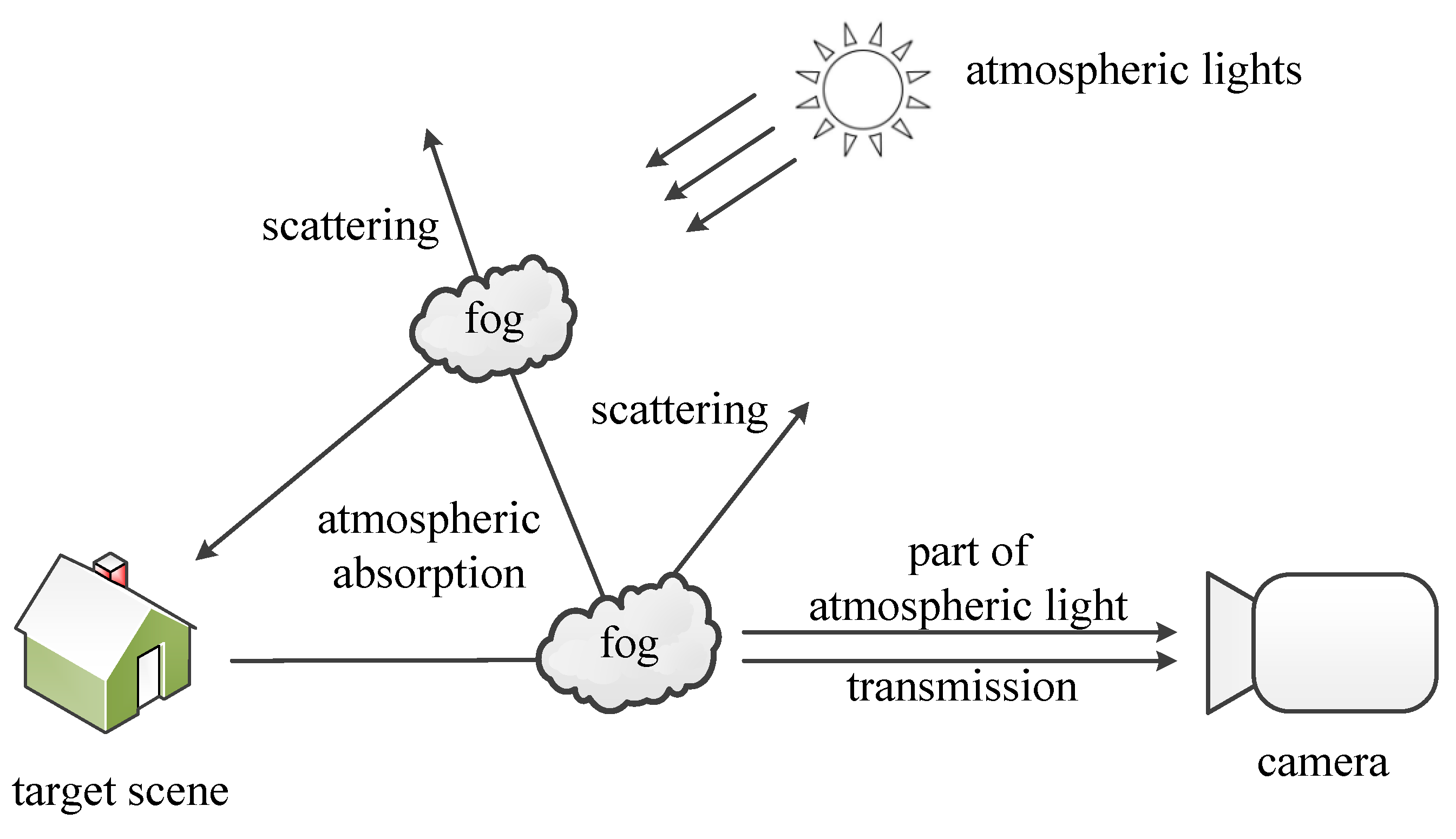
2.1. Haze Imaging Model

In computer vision and computer graphics, the haze imaging model generated according to the principles of the atmospheric scattering model is widely used, as shown in Figure 1, the physical model widely used to describe the formation of a haze image is as the following Equations (1)–(3):

$$I(x)=J(x)t(x)+A(1-t(x))$$

(1)

where $I$ is the observed intensity, $J$ is the original scene radiance, $A$ is the global atmospheric light, and $t$ is the medium transmission rate. The process of haze removal is to restore $J(x)$ from $I$ by estimating the scene parameter given by $A$ and $t(x)$.

Figure 1. Haze imaging model.

2.2. Dark Channel Prior

The dark channel prior [3] is based on statistics and observations on haze-free outdoor images. For most of the non-sky patches of haze-free images, some pixels always have pretty low intensity in at least one color channel. These dark spots are caused by those bright or dim colored objects and scenery shadows in the real scene. For an image $J$, a dark channel is defined as:

$$J^{dark}\left(x\right)={\min }_{c\in \left\{r,g,b\right\}}\left({\min }_{y\in \mathsf{\Omega }\left(x\right)}\left(J^c\left(y\right)\right)\right)$$

(2)

where $J^c$ is one color channel of image $J$, $\mathsf{\Omega }(x)$ is a local patch centered at $x$. According to the concept of DCP, the intensity of dark channel $J^{dark}$ is extremely low and tends to be zero except for the sky scenery if $J$ is a haze-free outdoor image [5].

Due to the additive scattering air light, the hazy images typically have larger pixel values in those areas where the transmission is small. The dark channel of the haze image hsas higher intensity than its original value in regions covered by the dense haze. It can be visually interpreted that the dark channel intensity of the haze image is a rough approximation of the haze concentration [5].

2.3. Algorithm Flow

In this method, a guided filter is used instead of the procedure to estimate and refine the transmission map of haze images. The basic algorithm flow of haze removal based on DCP is as follows; the input haze image is defined as I:

(1)

Calculate the grayscale image $I_{gray}$ with:

$$I_{gray}=0.299\times I_{red}+0.587\times I_{green}+0.114\times I_{blue}$$

(3)

(2)

Calculate the dark channel $I^{dark}$ by Equation (2).

(3)

Estimate the global atmospheric light $A$ based on the input haze image and its dark channel map. First, we index the position of the brightest 0.1% pixels in the dark channel map. Then, we calculate the average value of the pixels in these locations in $I$ as the atmospheric light $A$.

(4)

Assume that the value of scenery transmission remains as a constant in a local patch $\mathsf{\Omega }\left(x\right)$ and define the transmission as $\tilde{t}\left(x\right)$. According to the haze imaging model and the dark channel prior, we obtain the initial transmission with:

$$\tilde{t}\left(x\right)=1-\omega {min}_c\left({min}_{y\in \mathsf{\Omega }\left(x\right)}\frac{I^c\left(y\right)}{A^c}\right)$$

(4)

where the patch size is typically $15\times 15$. The variable $\omega$ is introduced into the transmission equation above to maintain the effect of depth and reality [3]. In order to reserve a small portion of haze for the remote scene in the image, we set $\omega$ to 0.95 in this paper.

(5)

The guided filtering is performed on the initial transmission $\tilde{t}(x)$ with the gray image as the guidance image and obtain the refined transmission $t(x)$. The soft matting algorithm is replaced in this paper due to its computing complexity.

(6)

To reduce the color distortion, the transmission [25] is adjusted for the bright areas with tolerances $K$:

$$t(x)=\{\begin{array}{ll}t(x)& \left|A-I(x)\right|>K\\ \frac{K}{\left|A-I(x)\right|}·t(x)& \left|A-I(x)\right|\le K\end{array}$$

(5)

The value of $K$ is set to 80 in our experiments.

(7)

Based on the atmospheric light $A$ and transmission $t(x)$, we can restore the clear image by Equation (6). Given the transmission $t(x)$, a minimum limit $t_0=0.1$.

$$J\left(x\right)=\frac{I\left(x\right)-A}{\max \left(t\left(x\right),t_0\right)}+A$$

(6)

Since the atmospheric light is usually brighter than the scene radiance, the image after haze removal appears darker. Meanwhile, due to the approximate estimation, the scenery transmission is relatively small, causing the value of pixels to be smaller. So, we increase the brightness of $J(x)$:

$$J^c(x)=J(x)+(1-J(x))\times J(x)\times B$$

(7)

where B is a brightness factor, takes 0.2 as in [25].

The results obtained by the above algorithm are shown in Figure 2.

Figure 2. Haze removal results. (a) Original images with haze. (b) Initial transmission maps. (c) Refined transmission maps after guided filter. (d) Recovered haze-free images by our method.

The time-consuming ratio of each module in the haze removal algorithm evaluated on a single thread CPU platform is shown in Figure 3. As we can see from Figure 3, the most time-consuming section is the dark channel calculation and transmission calculation.

Figure 3. The time-consuming ratio.

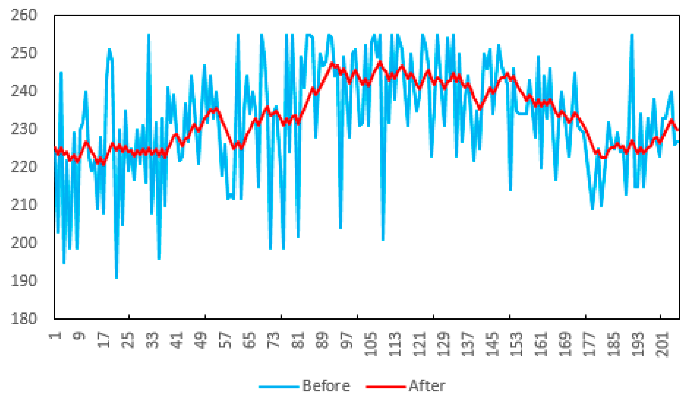
2.4. Atmospheric Light Optimization

A single image haze removal algorithm can obtain a high-quality clear image. However, if the single image haze removal algorithm is directly used in video processing, it will cause severe video flicker. We found that atmospheric light is the main reason for video flicker. If the atmospheric light between adjacent frames varies by a value larger than 5, we will notice video flicker obviously. We propose an inter-frame atmospheric light constraint algorithm to smooth the inter-frame skewing.

$$A^{\prime }=A_p\pm (diffm-\frac{\left|diff\right|}{2^{n+1}})$$

(8)

where $A^{\prime }$ is the adjusted atmospheric light, $A_p$ is the atmospheric light before adjustment, and $diffm$ is the maximum allowable atmospheric light difference between two adjacent frames. The calculated difference in atmospheric light difference between the current frame and the previous frame determines $+$ or $-$. If $diff$ is positive, it takes $+$; otherwise, it takes $-$. The coefficient $n$ is the multiple of the actual difference and the maximum difference.

3. GPU-Accelerated Implementation for Image Haze Removal Based on Dark Channel Prior

In this section, the parallel strategy based on the algorithm flow in the last section is discussed. We parallel implement each step of the haze removal algorithm to achieve real-time processing.

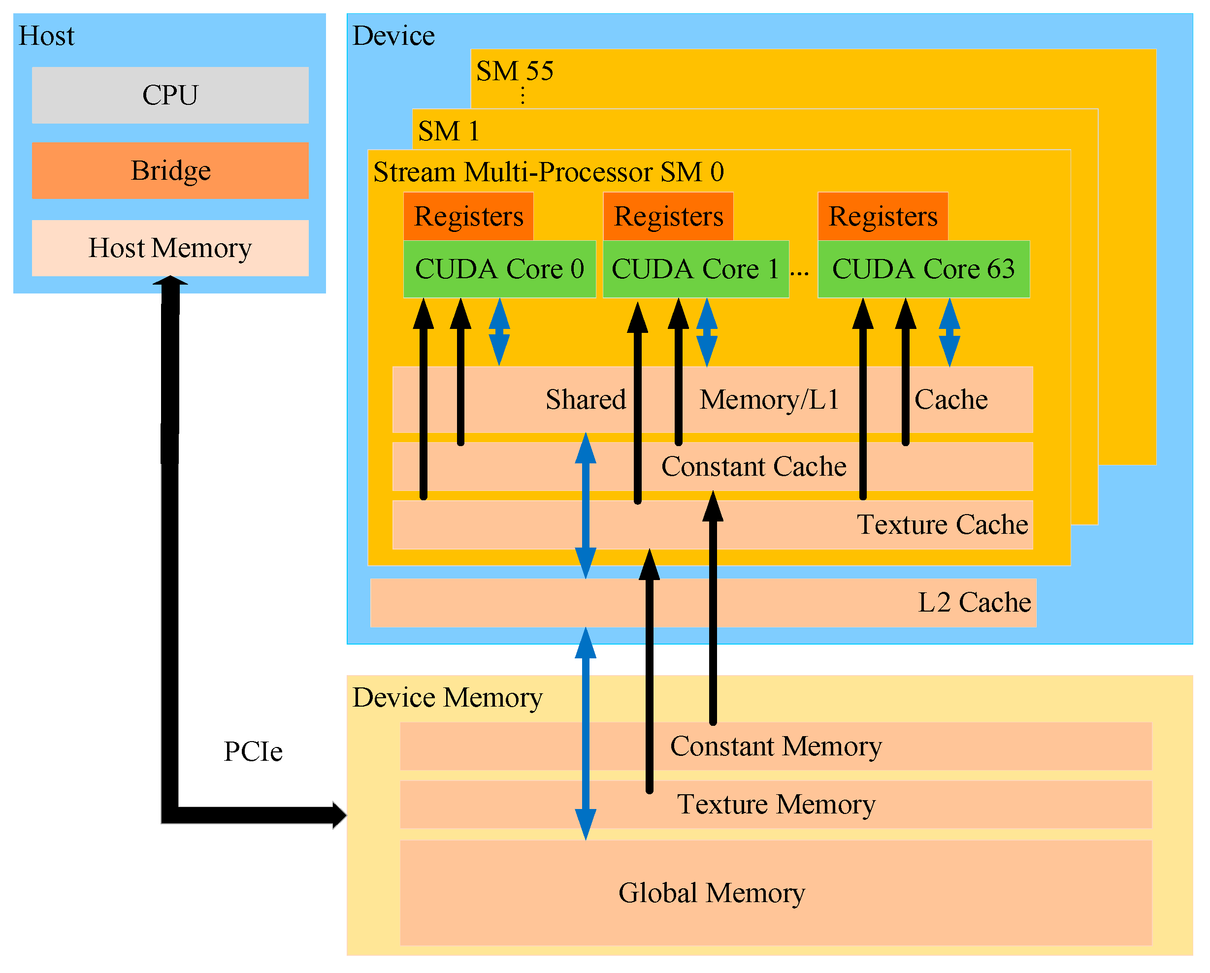
3.1. General GPU Parallel-Computing

Nowadays, GPUs (Graphic Processing Units) play an increasingly important role in the field of high-performance computing due to their massive-threads computing architecture and excellent floating-point computing capability. Numerous threads are launched to conceal the memory access latency with remarkably streamed controlling logic [5,17].

A CUDA (Computed Unified Device Architecture) parallel programming model was developed by NVIDIA to accelerate GPU programming. The CPU is suitable for handling complex control-intensive tasks while the GPU is suitable for processing computing-intensive tasks. The complementary feature of CPU and GPU facilitates the development of heterogeneous computing architectures. With the development of large-scale computing research, such as deep learning, big data, etc., the application of GPU is also developing rapidly.

The experiments in this paper are evaluated on four GPU platforms: Tesla C2075, Tesla K80, GeForce GTX 1080 Ti, and GeForce RTX 2080 Ti. The detail parameters are shown in Table 1. GeForce RTX 2080 Ti uses the Turing architecture with a computing capability of 7.5. GeForce GTX 1080 Ti uses Pascal architecture with a computing capability of 6.1. The K80 uses dual-core GPUs based on Kepler architecture. The C2075 uses Fermi architecture. All GPU devices support memory allocation requirements for high-resolution image calculations. The deep optimized parallel haze removal algorithm combined with the appropriate allocation of memory can fully accelerate the performance of the kernel functions.

Table 1. Tesla C2075, Tesla K80, and GeForce GTX 1080 Ti Performance Parameters.

Name	Cores (MP)	Memory Size(GB)	Architecture	Capability
C2075	448	6	Fermi 2.0	2.0
K80	2496	12	Kepler	3.7
GTX 1080 Ti	3584	12	Pascal	6.1
RTX 2080 Ti	4352	12	Turing	7.5

GPU has different memory hierarchies, with different scopes, accessing clock cycles and caching behaviors. The GPU memory hierarchies of NVIDIA Pascal architecture are shown in Figure 4. The GPU memory architecture mainly includes register, shared memory, local memory, constant memory, and global memory. The register is the fastest on the GPU. Global memory is the largest and most common used memory in the GPU, but typically takes hundreds of clock cycles to access. It can be accessed by any thread at any time during the kernel execution. Shared memory, similar to L1 cache, has higher bandwidth and lower latency. Constant and texture memory can be accelerated through the specified read-only cache.

Figure 4. Graphics Processing Unit (GPU) memory architecture of NVIDIA Pascal architecture.

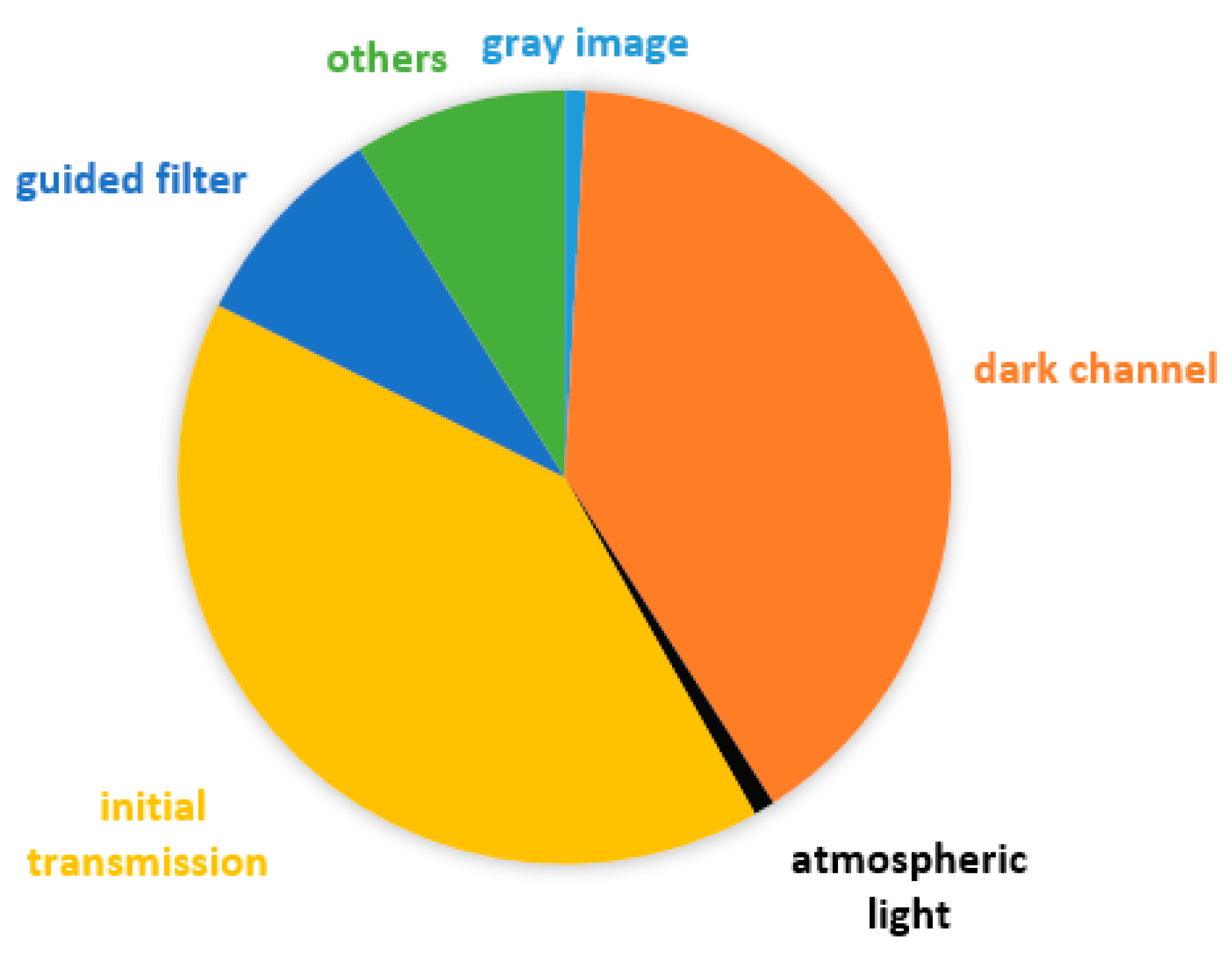
3.2. The Time-Consuming Part

The most time-consuming parts are channel calculation and transmission calculation. The minimum filter is used to calculate the dark channel and initial transmission. The major process of the guided filter is the mean filter. So, the most time-consuming part is the minimum filter and the mean filter.

GPU accesses contiguous addresses faster than intermittent memory addresses in global memory. Based on this feature and the computational characteristics of the GPU, we propose a transposed filter algorithm. Instead of using a two-dimensional convolution kernel, we use a one-dimensional convolution kernel. First, the image or the two-dimensional matrix is subjected to row-direction filtering. This filter box is a one-dimensional filter box, and the filter box size is $2\times r+1$ ($r$ is the radius of the filter box). Then, the image or matrix is transposed to swap the rows and columns. Now the new image is subjected to the previous row-direction filtering operation and transposed. Finally, we get the corresponding filtering results.

Figure 5 shows the entire transposed filter algorithm. In the following, we describe the mean and minimum filter used in our dehazing algorithm.

Figure 5. Transposed filter algorithm.

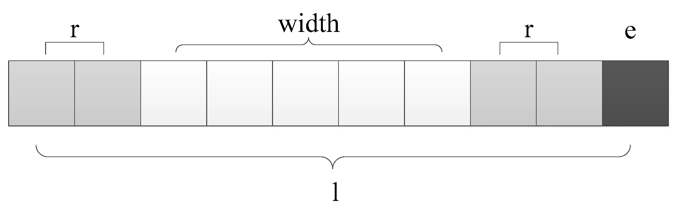
3.2.1. The Minimum Filter

In the process of realizing the haze removal algorithm, Equations (2) and (4) indicate that in generating a dark channel map and the initial transmission estimation a minimum neighborhood computation is required for the input haze image and its normalized image. This means we need to process a minimum filter to the image. In the entire haze removal algorithm, the minimum filter is invoked twice, and its time complexity greatly limits the speed of the entire program. In order to reduce the calculation of the minimum filter, a row and column-independent process is put forward to guide the minimum filter in this paper. The detailed algorithm process is shown in Figure 6.

Figure 6. Schematic diagram of the minimum filter algorithm (r = 1).

As shown in Figure 6, each result of the original algorithm requires ${(2\times r+1)}^2-1$ compare operations. The one-dimensional filter of the new algorithm requires $(2\times r+1)-1$ compare operations, but it requires two filtering on rows and columns directions, individually. However, the time complexity of the algorithm is still highly correlated with the size of the filter kernel $r$. If we use the fast local minimum algorithm [17], the computational complexity is reduced and finally it takes only six calculation iterations to figure out the filtered results for all elements. Its time complexity is independent of the filter kernel size $r$, so it has great advantages in reducing the computation payload.

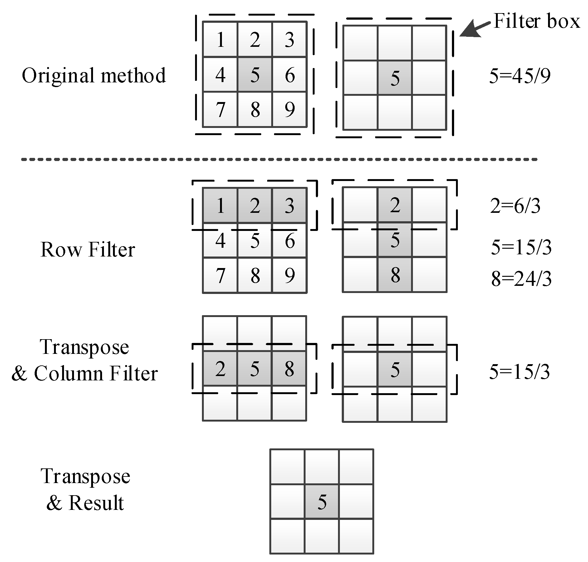
3.2.2. The Mean Filter

In the guided filter, the mean filter takes a large proportion of the algorithm complexity. So, optimization for the mean filter is the key point. The mean filter is a linear filter, and its processing is very simple. The average value of the pixels in a window area is calculated, and then the average value calculated is set to the pixel value on the center position of the window. The results of two adjacent locations with $n\times (n-1)$ data are calculated repeatedly ($n$ is the size of the filter box).

Data reusage can improve the mean filter greatly with row and column processing, separately. The method is shown in Figure 7. In this algorithm, the results of two adjacent positions with $(n-1)$ data are calculated repeatedly. Even if one-dimensional mean filtering needs to be calculated twice, the repeated data of two adjacent positions is only $(n-1)\times 2$. In addition, we also use the integral image [29] to further reduce data reusage and accelerate the mean filtering.

Figure 7. Schematic diagram of the mean filter algorithm (r = 1).

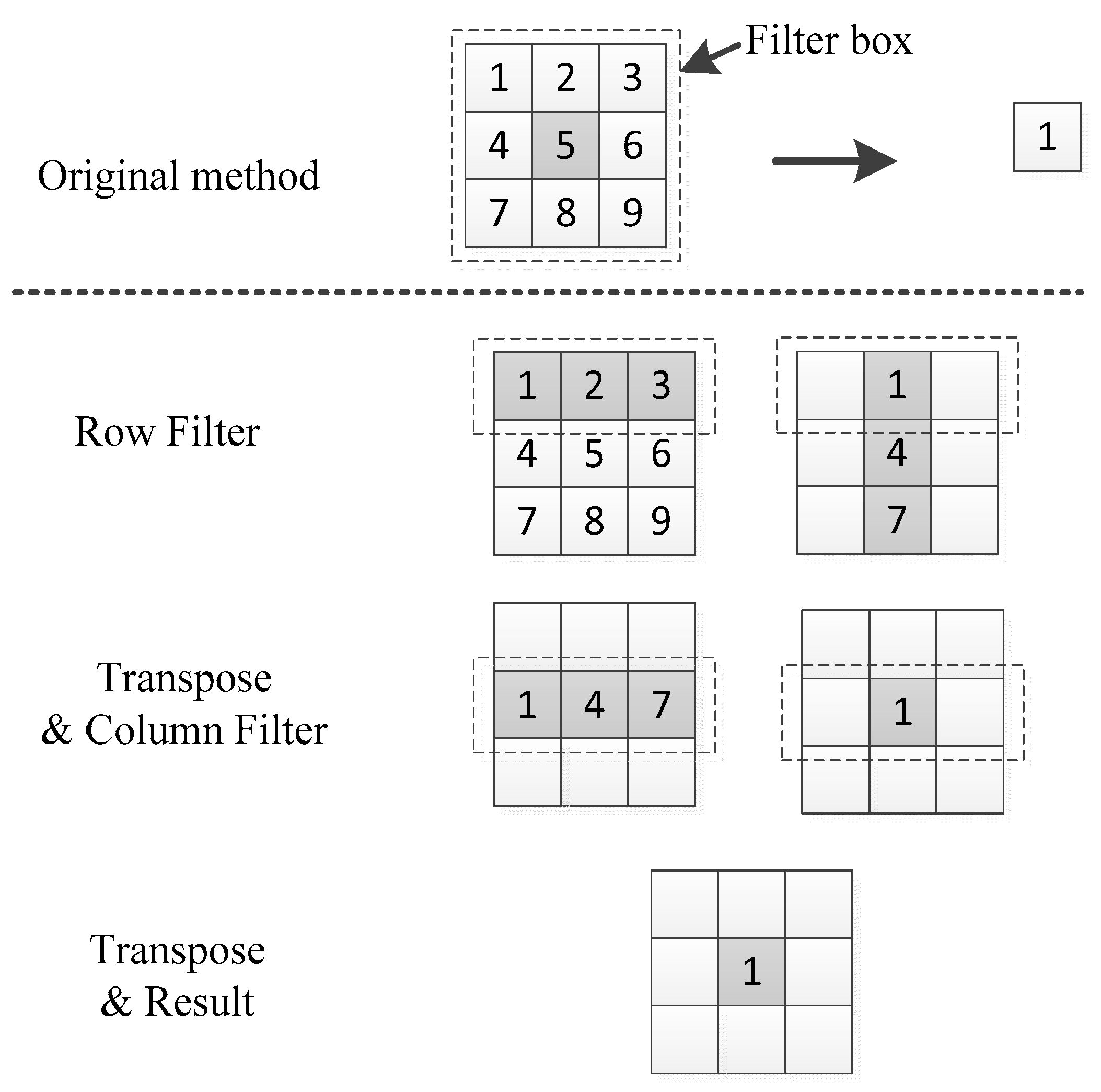
3.3. Transposed Filter Algorithm Based on GPU

In traditional implementations [10,11,12,13,14,35,36], row and column filtering are performed separately. However, we found that during the mean filter for an image [37] in column direction, threads in each warp act with an integrated access pattern when executing the same instruction and perform very fast. However, when the filter is in row direction, threads act with a discontinuous access pattern, even when executing the same instruction, and bring huge latency.

Inspired by the filtering efficiency in the column direction, a transposed filter is proposed in this paper to improve parallel processing efficiency in GPU. The proposed transposed filter is based on the feature that the GPU performs better when accessing contiguous memory addresses. In this section, we will introduce the specific implementation of filters.

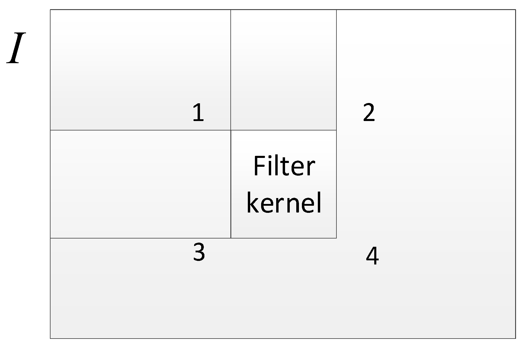
3.3.1. Transposed Filter Algorithm

After filtering the rows of the image, we transpose the image results, so that we can use the same filtering kernel twice to get the filtered image. After the column items are calculated, we transpose the results again to recover the normal image (https://github.com/wuxianyun/DCP_Dehaze_GPU_CUDA).

In order to reduce the time of transposition, we use the shared memory along with the coalesced memory access and apply padding to the shared memory to avoid bank conflicts [37].

3.3.2. Parallel Minimum Filter Algorithm

In the traditional minimum filter algorithm, there is a great amount of data multiplexing in adjacent pixels. Therefore, it is possible to increase the data reusing rate to improve the efficiency of the algorithm.

The local minimum/maximum fast filtering [16] proposed by Van Herk M is an algorithm that fully considers data multiplexing and has a computational complexity of only O(N). Recursive procedures (9) and (10) and operation (11) describe the whole algorithm:

$$g_x=\{\begin{array}{ll}{f}_x& for x=1, k+1, 2k+1,\dots \\ \min \left[g_{x-1}, f_x\right]& \begin{array}{c}for x=2,\dots , k; k+2, \dots , 2k;\\ 2k+2, \dots 3k;\dots \end{array}\end{array}$$

(9)

$$h_x=\{\begin{array}{ll}{f}_x& for x=N, N-k-1, N-2k-1,\dots \\ \min \left[{\mathrm{h}}_{x+1}, f_x\right]& \begin{array}{c}for x=N-1,\dots , N-k;\\ N-k-2, \dots ,N-2k-1;\dots \end{array}\end{array}$$

(10)

$$Resul{t}_x=min\left[g_{x+\left(k-1\right)/2}, h_{x-\left(k-1\right)/2}\right] for x=1,\dots , N$$

(11)

where $k$ is the size of the filter box. The input array $f$ is divided into sub-arrays (groups) of size $k$. In each sub-array, we perform the same operation as follows. The i-th value of the sub-arrays, stored in the matrix $g$, is the minimum value of the first i pixels of each sub-array of the input matrix $f$. The (k + 1 − i)-th value of the sub-arrays, stored in the matrix $h$, is the minimum value of the last i pixel of each sub-array of the input matrix $f$. By comparing the value $h_{x-(k-1)/2}$ with the value $g_{x+(k-1)/2}$, we can get the minimum value Result_x as shown in Figure 8.

Figure 8. Local minimum filter algorithm. The parameter is k = 5. A symbol ‘←’ denotes that the value is the minimum of all values covered by that arrow.

For the one-dimensional direction, the entire operation only requires three operations for each element. For the entire image the local minimum filter process needs to perform three operations for each pixel in the row and column direction; that is, each pixel only needs six operations. The final result can be obtained no matter the size of the filter kernel.

To avoid the boundary overflow in Equation (11), we need to perform a boundary determination for all elements. In this paper, we use the method of boundary padding to avoid the boundary determination and improve the efficiency of the algorithm. During this process, the data is directly stored in the shared memory, which further improves the efficiency of the algorithm by increasing the speed of memory access.

In the minimum filter, the fill value is 255 and the filling procedure is shown in Figure 9. First, we add $r$ (radius of the filter box) elements on both sides of each row of elements. Then, we add $e$ elements to the end of the array. So that the new vector size $l$ is an integer multiple of the filter box size $mask$.

$$mask=2\times r+1$$

(12)

$$e=mask-(witdth+2\times r)\%mask$$

(13)

$$l=witdth+2\times r+e$$

(14)

Figure 9. Minimum filter boundary fill.

When programming with CUDA [36,37,38,39], we set a thread block for each row/column of the image, and 128 threads for each thread block in this paper. There is a dependence on adjacent points in the sub-array range when we calculate the arrays $g$ and $h$, so one thread is used to process one sub-array, and multiple threads process in parallel. When calculating the $result$ array, since all pixel calculations are independent of each other, we configure one single thread to process one single pixel, while we use multiple threads for processing in parallel.

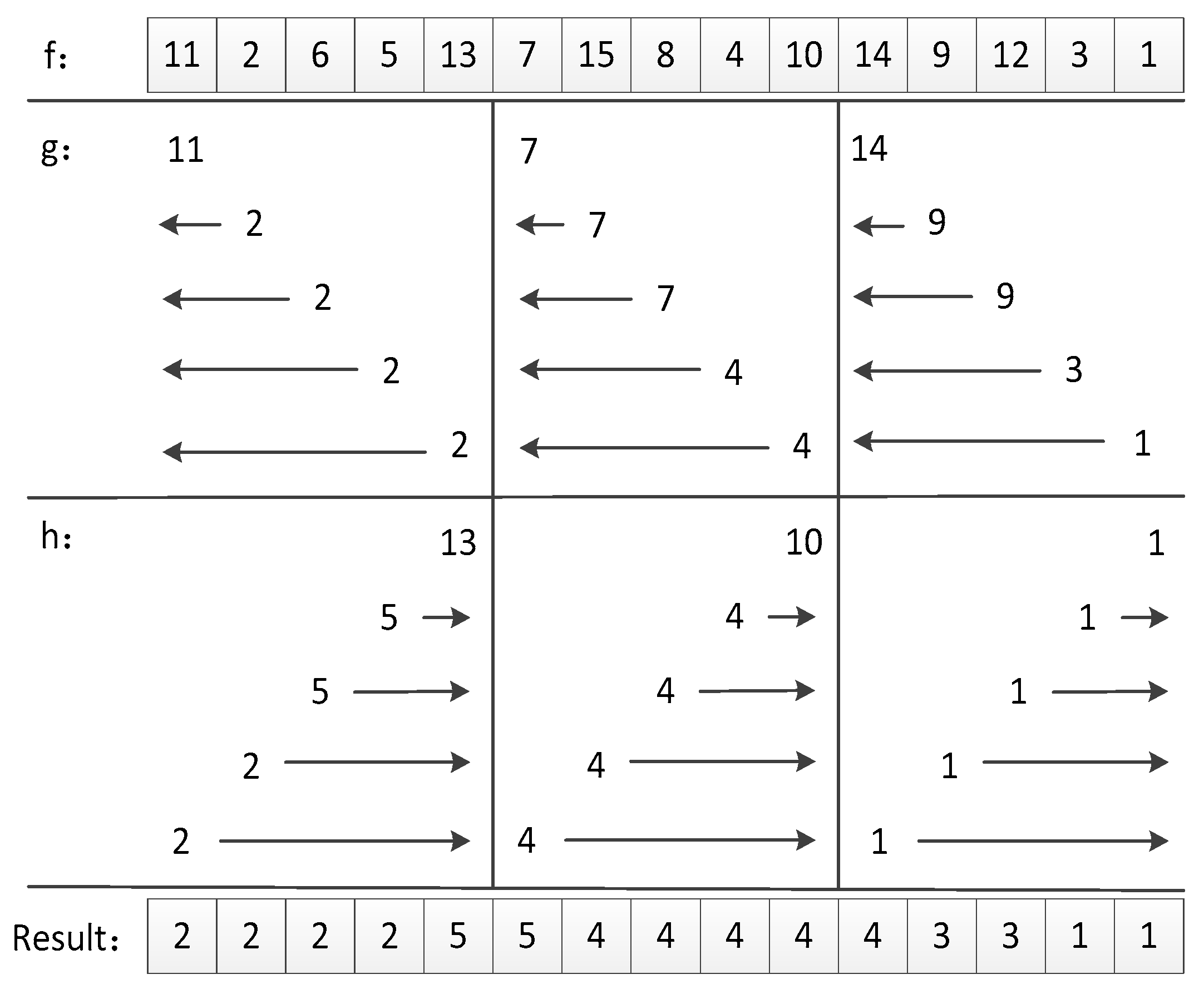
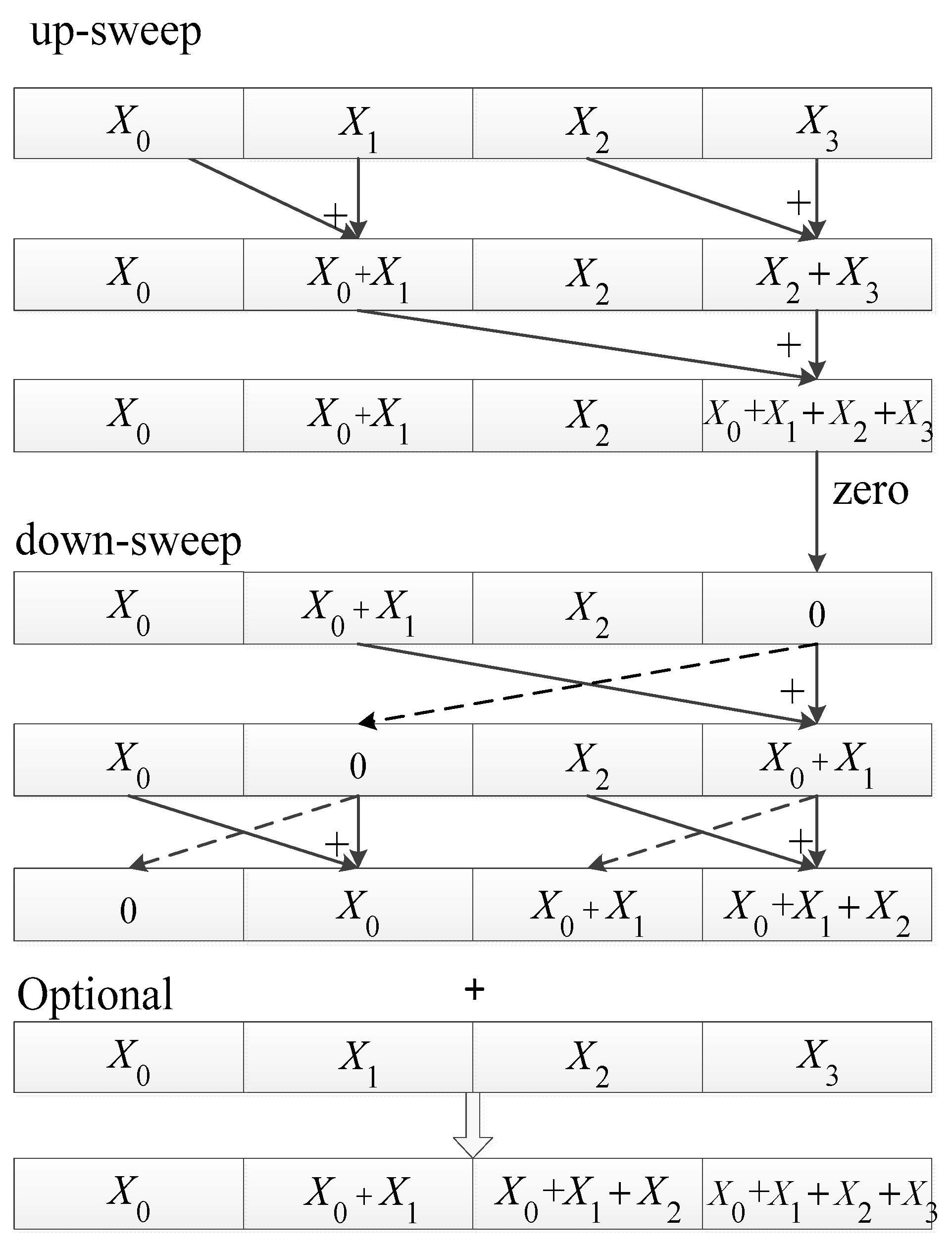
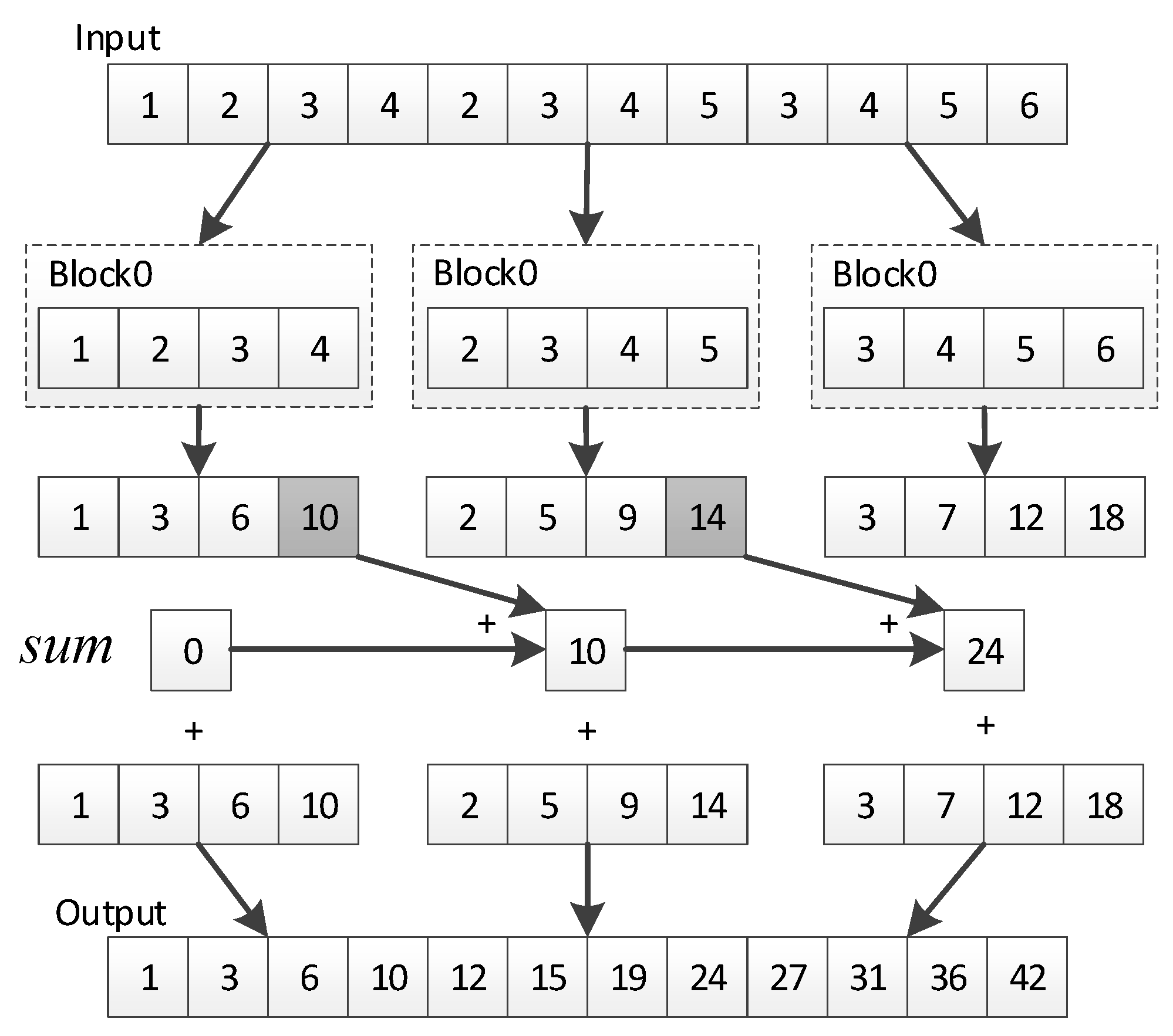
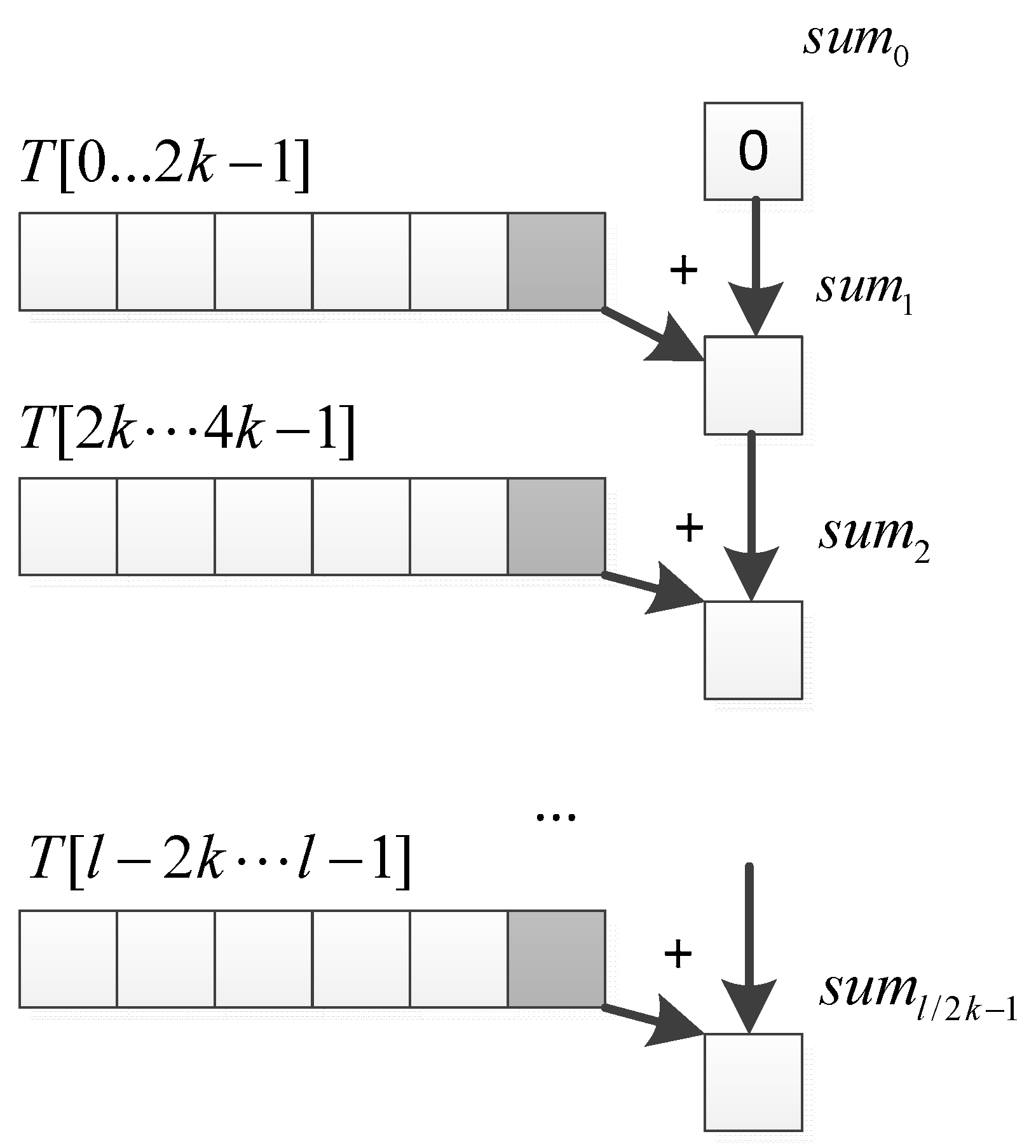
3.3.3. Parallel Mean Filter Algorithm Based on Scan

In the mean filter, there is also a great amount of data multiplexing in adjacent pixels. Therefore, it is still important to improve the data reuse for the parallel algorithm.

The average value is the sum of all the elements in the area divided by the number of elements. The size of the filter kernel is fixed, so we focus on improving the efficiency of pixel summation within the filter box.

The integral image algorithm [37] proposed by Viola and Jones is widely used in face recognition algorithms. The concept of integral image is similar to the area of local neighborhood in mathematics. We can get an integral image with:

$$ii(x,y)={\displaystyle \sum _{0\le x^{\prime }\le x,0\le y^{\prime }\le y}i(x^{\prime },y^{\prime })}$$

(15)

where $ii(x,y)$ is the integral image value at location $(x,y)$ and $i(x,y)$ is the input image.

We assume that the filter kernel position is shown in Figure 10 when calculating the center point, and we calculate the sum of all pixels in the filter kernel with:

$$su{m}_{box}=i{i}_{rightbottom}-i{i}_{righttop}-i{i}_{leftbottom}+i{i}_{lefttop}$$

(16)

Figure 10. The sum of pixels in the filter kernel.

In 2010, Bilgic B et al. proposed an efficient parallel algorithm for real-time calculation of integral images [27]. This algorithm is based on the Parallel Prefix Sum (Scan), a very classic algorithm in the field of parallel computing. The specific process is shown in Figure 11.

Figure 11. Parallel prefix sum (Scan). This is an inclusive scan operation, and the operation before optional is an exclusive scan operation.

If the input one-dimensional array size is $n$, the time complexity of the scan algorithm is $O(n)$. This algorithm consists of two parts, the reduce phase (or the up-sweep phase) and the down-sweep phase. In the reduce phase, we reduce the number of nodes by half at each level. In the down-sweep phase, we first set the last element to zero, then we sum elements and swap their positions until the zero propagates to reach the beginning of the array, thus getting an exclusive scan result. The computational complexity of the algorithm is $2\times (n-1)$ additions and $(n-1)$ swaps, whose time complexity is $O(n)$, the same as the sequential algorithm.

All computational operations are performed in shared memory to ensure the algorithm efficiency. When the input is an image, combined with the transposed filter algorithm, we perform the parallel prefix sum operation on the rows of the image first, then transpose, and then apply the parallel prefix sum again on the rows of the transposed image.

The computational complexity of the parallel algorithm is $O(n)$, and we use data partitioning to further reduce the time consumption. As we can see from Figure 11, in the parallel prefix sum algorithm, the length of the input array must be $2^n$. In order to improve the compatibility of the parallel algorithm without being limited by the size of the input array, we adopt the method in [36]. In this algorithm, multiple thread blocks are not specified, and each thread block is responsible for a portion of the data rather than the entire data. As shown in Figure 12, if the input data length is $n$ and each block is responsible for the calculation of $m$ data, $n/m$ thread blocks are needed to be opened and $m/2$ threads are allocated for each block. During the scanning process, thread blocks are independent of each other and do not interact with each other. After the parallel prefix sum of each submatrix, the last element in each block is recorded in an extra array $su{m}_i$, which is the sum of all elements before the i-th block. Then we add $su{m}_i$ to all the elements in the i-th block to get the scan result.

Figure 12. Multi-block scan. The parameters are three blocks, $n=12$, $m=4$.

In Huang’s method, we need to set multiple thread blocks to calculate each submatrix [39]. The calculations between different blocks are independent of each other and the results are not accessible between different blocks. Therefore, in order to obtain the results of the integral image, we need to allocate global memory to store the $sum$ array. We must wait for all intra-block calculations to be completed and then calculate the average of each filter kernel. This means two kernel functions need to be invoked to implement a one-dimensional mean filter; one kernel is used to calculate the parallel prefix sum and the other kernel is used to calculate the mean value. This approach results in extra computation and unnecessary I/O access to global memory, which greatly increase the run time and reduce the efficiency of the algorithm.

The implementation of the mean filter using an integral image is further improved in this paper. We still use a transposed filter to separate the rows and columns, and use a one thread block to process one line of the image. For all calculations of the one-dimensional filter kernel, we use shared memory to reduce data access latency. We assume that the resolution of the input image is $w\times h$ and the filter kernel radius is $r$. The specific implementation scheme of a one-dimensional filter kernel is as follows:

Step 1. Kernel function parameter setting. Launch $h$ (the number of rows of the input image) blocks; one block processes one line of image. Allocate $h$ threads in each thread block ($k$ meets the size $2^n$ and $k\le 1024$). These $k$ threads can process $2\times k$ data at a time.

Step 2. Bound extension. In the mean filter, the boundary determination of the image can cause warp diversion. In order to avoid warp diversion on the warp schedule in the GPU, it is necessary to perform a bound extension operation on the image. The extension operation is similar to the minimum filter bound extension of Figure 9. Firstly, we fill $r$ elements on both sides of the one-dimensional array ($r$ is the filter kernel radius). Then we add e elements to the end of the array, and make sure that the filled array width $l$ is an integer multiple of $2\times k$. We fill the first element of the array in front of the array and the last element of the array after the array. When bound extension is finished, the input image is directly loaded from the global memory into the shared memory T, and the shared memory size allocated for each block is $l$.

$$l=\lceil (w+2\times r+2\times k)/(2\times k)\rceil \times 2\times k$$

(17)

$$e=l-(w+2\times r)$$

(18)

Step 3. Parallel prefix sum [39]. Each block uses the data in shared memory $T$ for calculation. Since $k$ threads process $2\times k$ data at a time, all data in each thread block are divided into a $l/(2\times k)$ sub-matrix. The parallel prefix sum result can be obtained by iterating $l/(2\times k)$ times with $k$ threads. We use the exclusive scan shown in Figure 11, and we allocate shared memory $su{m}_i$ of size $l/(2\times k)$ in each thread block to store the sum of all pixels before the sub-matrix $i$, as shown in Figure 13.

$$su{m}_0=0$$

(19)

$$su{m}_i=su{m}_{i-1}+T\left[i\times k\times 2-1\right]$$

(20)

Figure 13. The parallel prefix sum in each block.

Step 4. Mean filter. The result of the parallel prefix sum is equivalent to obtaining the one-dimensional integral image of the rows or columns. The calculation method of the mean filter result of the i-th one-dimensional filter kernel of any row is as follows. The one-dimensional array scan results are recorded in the $box$ array, and the $bo{x}_i$ represents the sum of the first to i-th pixels. The filter kernel size is $mask=2\times r+1$. The mean filtering result is recorded in $result$.

$$bo{x}_{i+r}=T\left[i+r\right]+sum\left[\lceil \frac{i+r}{2\times k}\rceil \right]$$

(21)

$$bo{x}_{i-r-1}=T\left[i-r-1\right]+sum\left[\lceil \frac{i-r-1}{2\times k}\rceil \right]$$

(22)

$$resul{t}_i=\frac{bo{x}_{i+r}-bo{x}_{i-r-1}}{2\times r+1}$$

(23)

Before the parallel prefix sum, we need to extend the array to avoid unnecessary calculations. However, the larger the thread $k$ is set, the greater amount of unnecessary calculation, but if the $k$ is too small, GPU resources will be wasted. Therefore, a reasonable thread configuration is important to optimize the efficiency of the mean filter algorithm based on the integral image [35,36,40,41]. In this paper the thread number per block is set to 128 after evaluating a large number of experimental tests.

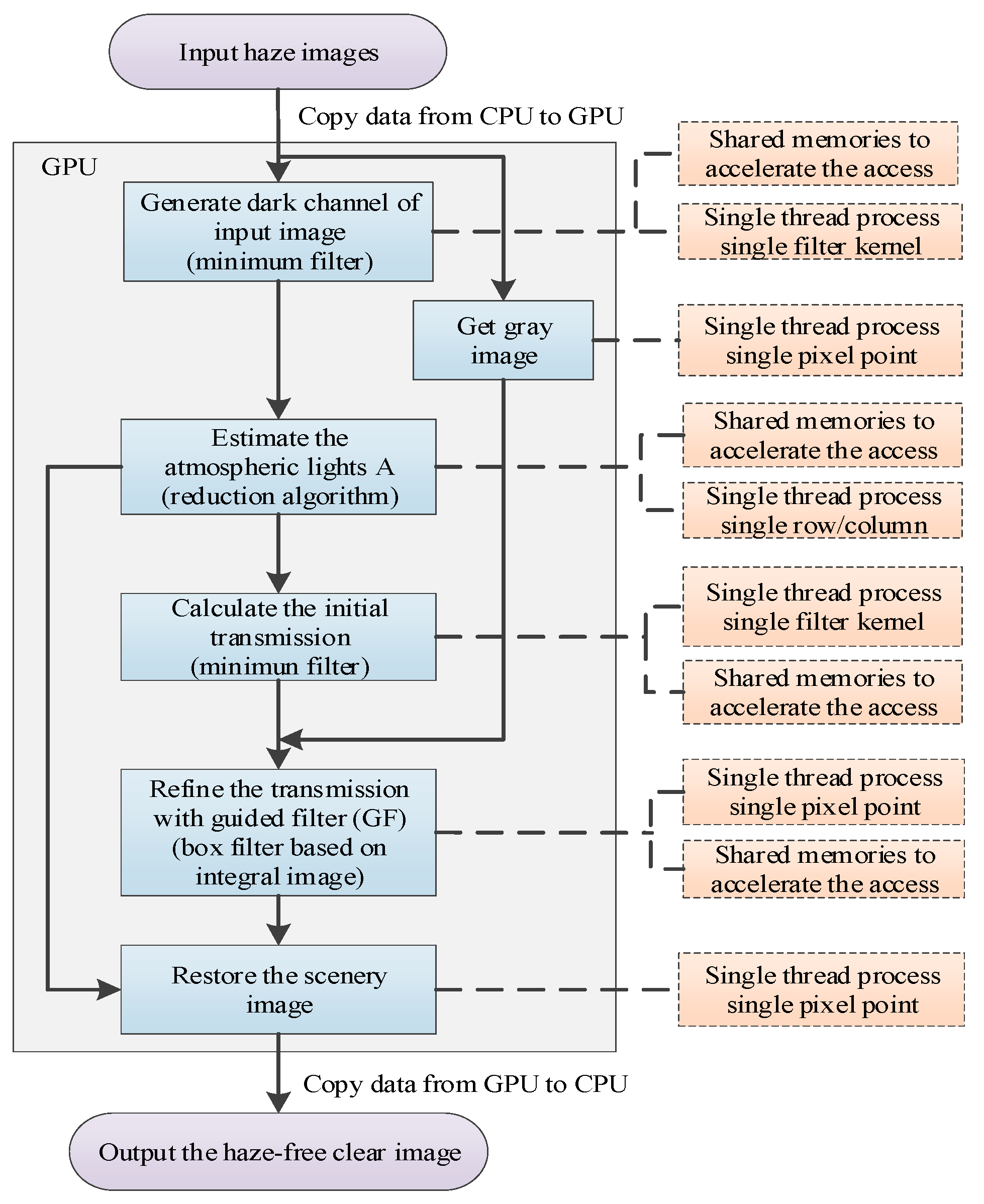
3.4. GPU Implementation of Dehazing Algorithm

In addition to the transpose-based filtering algorithm, we also use GPU-based optimization strategies such as reduction, scan, and shared memory to realize real-time processing of high-definition video images.

Based on the algorithm flow in Section 2, we implement the corresponding parallel computing strategy for each module in the entire algorithm. Memory transfer between host and device takes up a large part of the whole implementation. This is not important when processing a still image. However, in video processing, a large amount of data transmission is involved, and the latency caused by data transmission is obvious. We will present a method to solve this problem in the next section.

We set the size of filter kernel to $15\times 15$, which means that the r mentioned in this paper is equal to 7. We use the transpose-based minimum filter to obtain the dark channel map of the input haze image. In this procedure, there is a dependence on adjacent pixels in the sub-array range when we calculate the arrays $g$ and $h$. We use one thread to process one sub-array, and multiple threads process in parallel. However, when we get the final result, the pixels are independent of each other, so we set it so that one thread processes one pixel. In addition, for the purpose of reducing expenses of repeated data access and further accelerating the memory access, texture memory employing the clamp addressing mode [5] is used to access the enormous amount of computation data during the filtering procedure.

The estimation of atmospheric light $A$ is based on the reduction algorithm [17]. As shown in Section 2, we first pick the top 0.1% brightest pixels in the dark channel. This means that we need to perform sorting which is very difficult to parallel implement on GPU. Instead we propose a simplified maximum scanning method for image atmospheric light estimation. The video frame haze removal results are shown in Figure 14.

Figure 14. Video frame haze removal results.

If the resolution of the dark channel map is $w\times h$, we set 1024 pixels as a group, and then we use $\lceil w\times h/1024\rceil$ thread blocks process each pixel group separately. Each thread block processes 1024 data, now we can find the maximum value in each thread block and record the pixel position. The $\lceil w\times h/1024\rceil$ maximum values and position obtained by this method are approximate to the top 0.1% brightest pixels in the dark channel, which greatly improves the efficiency of atmospheric light estimation.

The guided filter needs to call 6 mean filters based on image transpose. And one mean filter requires two image transpose, which means that the image is transposed 12 times during the entire guided filter. For one 1080 p HD video frame, one transpose takes only about 0.3 ms on Tesla C2075, but calling 12 times will bring nearly 4ms of time overhead to the entire procedure. This may cause large delay in video processing and greatly limits the real-time processing of video.

By analyzing the guided filter algorithm, we simplify the implementation of the mean filter. Reduce the second transposed filter that used to transpose the image back to its original state. Now we get the intermediate results of row and column inversion in the guided filter, like $mea{n}_I$, $mea{n}_{It}$, ${\mathrm{var}}_I$ and ${\mathrm{var}}_{It}$. Therefore, the linear correlation coefficient matrices $a$ and $b$ are also transposed. However, after performing mean filtering on $a$ and $b$, the final result $t$ is flipped back to the corresponding state. In this way, by simplifying the mean filter algorithm, the image transpose is reduced from 12 times to 6 times, deeply improves the efficiency of the haze removal algorithm.

The GPU-accelerated parallel computing implementation of the entire algorithm, the memory optimization, and the thread configuration are shown in Figure 15. In addition, the scenery transmission adjustment and the image enhancement portion are not shown in the flowchart. Table 2 is the memory allocation and usage of the main kernel (One 1080 p frame consumes 23.73 M memory space). And some memory can be recycled multiple times during kernel execution.

Figure 15. The GPU-accelerated parallel computing implementation flowchart.

Table 2. Memory footprint of our haze removal.

		Mean Filter	Minimum Filter	Estimate A	Grey Image	Restore Image	Transposed Filter
global memory	fixed	16 M	16 M	34 M	8.4 M	14.4 M	8 M
	recycle	8 M	16 M	8 M	23.6 M	23.6 M	8 M
shared memory		8 K	16 K	2 K	--	--	1 k

3.5. Coalesced Global Memory Access

Coalesced access can increase the global memory access efficiency in GPU. To enable the coalesced memory access, we need to pad data to original data which will enlarge the data transmission size between host and device. CUDA supports cudaMallocPitch to pad the data automatically [42]. Using coalesced memory access reduces the GPU kernel execution time. The device-to-host data transfer time using coalesced memory access turns out to be much longer than for non-coalesced memory access.

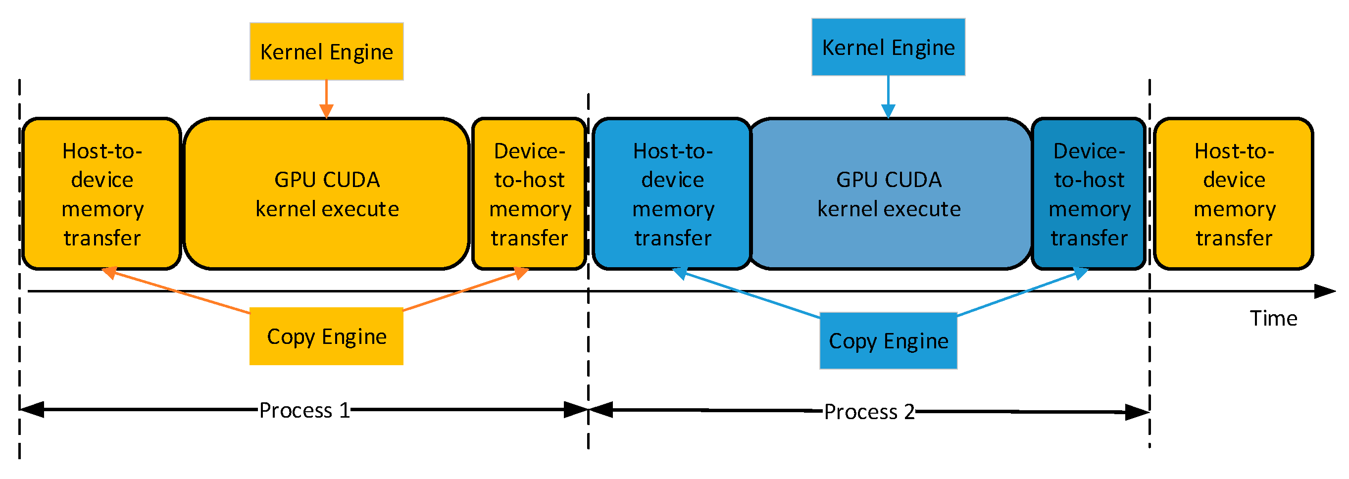
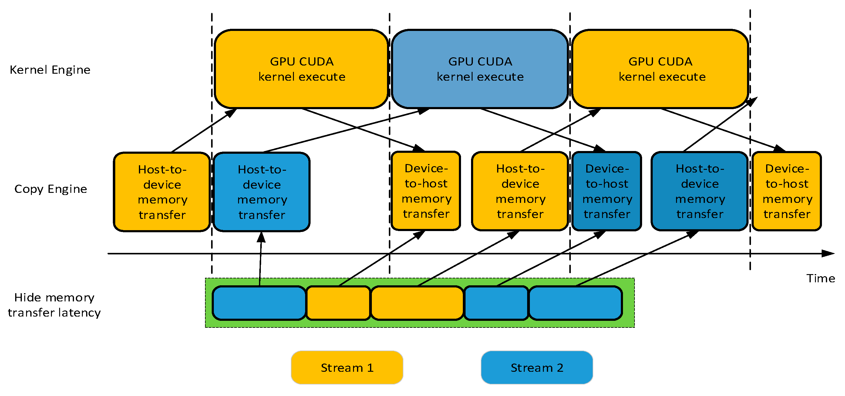
3.6. Asynchronous Memory Transfer

If we successively process the video frame, memory transfer between host and device will take up a large part of the whole implementation as shown in Figure 16. GPU can perform the data transfer engine with the computing kernel engine concurrently. I/O access time between CPU and GPU can be overlapped as shown in Figure 17, most of the data transfer between the CPU host and the GPU device is concealed.

Figure 16. Without using asynchronous memory access.

Figure 17. With asynchronous memory access.

We use two CUDA streams to hide the data transmission delay and reduce the GPU warm-up delay with asynchronous memory access. The accelerating result with asynchronous memory transfer is presented in next section. However, the transfer time of the first frame and the output time of the last frame are difficult conceal.

4. Experiments and Results Evaluation

In this section, we evaluate the high-performance parallel CUDA implementation algorithm based on the transposed filter described in Section 3 from subjective and objective quality. The GPU hardware platforms in this paper are NVDIA Tesla-C2075, NVDIA Tesla-K80, GeForce GTX 1080 Ti, and GeForce GTX 2080 Ti. The CPU platform is Intel(R) Core(TM) i5-3470 CPU @ 3.20GHz with 4GB RAM.

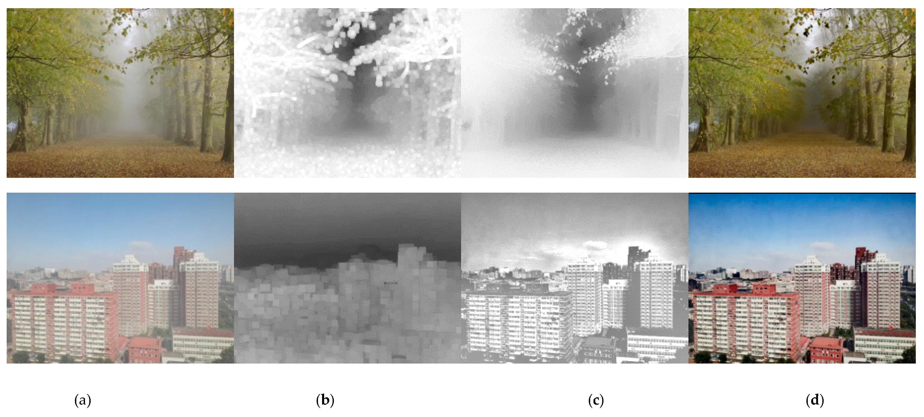
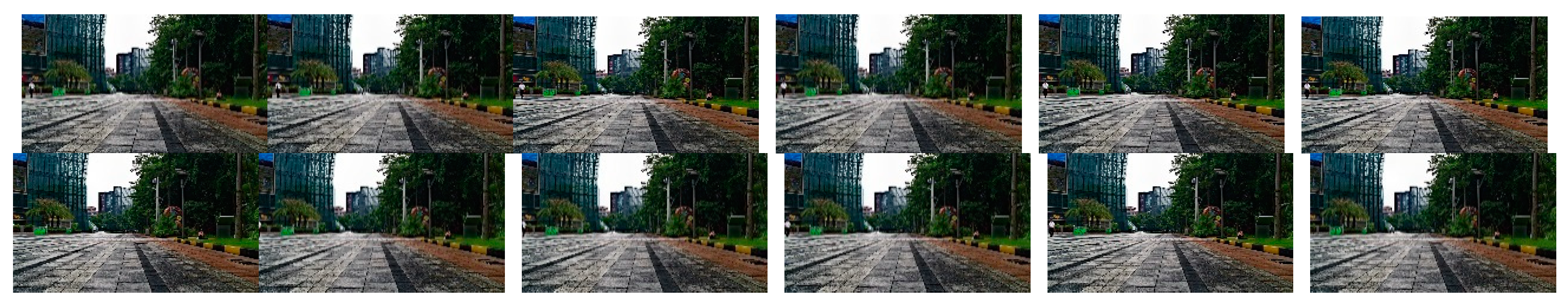
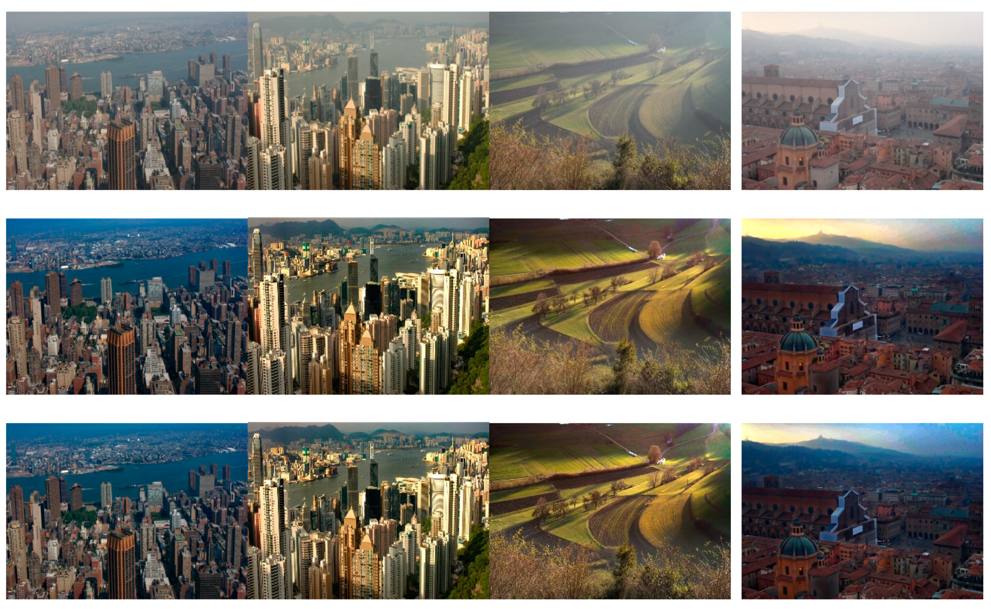
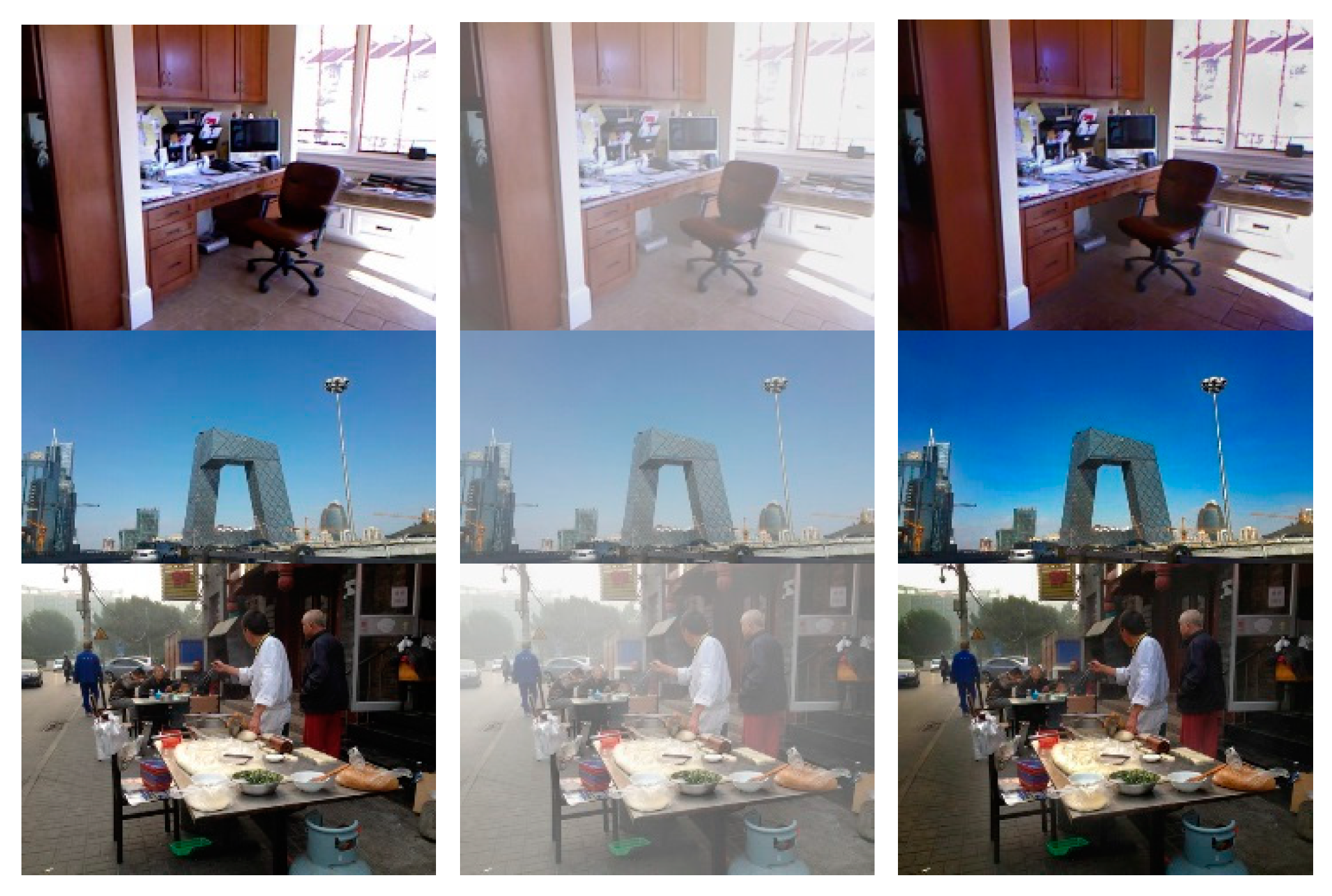
4.1. Effects of Haze Removal

Figure 14 shows the video processing results of several consecutive frames. The brightness between adjacent frames is smoothed as presented in Figure 18, and the video flicker is significantly suppressed. Figure 19 shows experiment results of the single image haze removal algorithm based on the transposed filter. The visual quality is equivalent to the current state-of-the-art dehaze algorithms [10,11,12,13,14,29,30,31,32,33,34], and even some details are brighter in color.

Figure 18. Atmospheric light value before and after adjustment.

Figure 19. Images with haze and after haze removal. Top: Original image with haze. Middle: Output image after haze removal on CPU. Bottom: Output image after haze removal on GPU.

In order to evaluate the performance of the inter-frame atmospheric light constraint, the atmospheric light values of 200 consecutive dehazing video frames were tested. As shown in Figure 18, the atmospheric light value of the algorithm in this paper is very stable, which shows that the proposed inter-frame atmospheric light constraint algorithm can efficiently adjust the atmospheric light value.

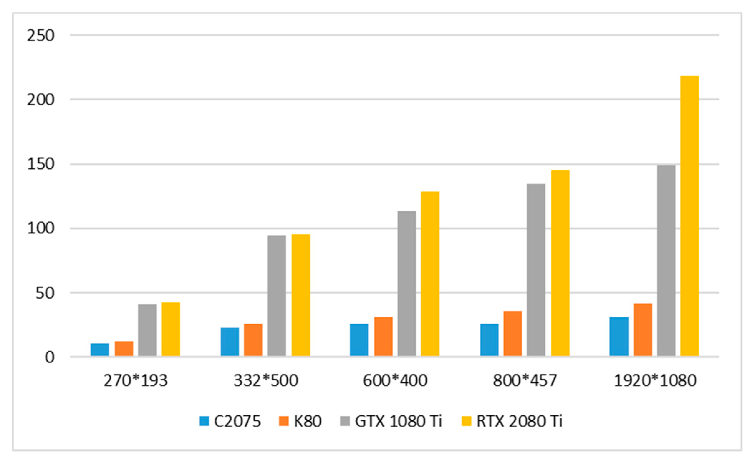
4.2. Algorithm Run Time Evaluation

To evaluate the accelerating efficiency of the parallel algorithm in this paper, we measured the running time of different image resolutions on CPU and GPU platforms. In order to reduce the random jitter, we timed ten times and took the average value as the final result. The results are shown in Table 3 and Table 4, Figure 20. As the image resolution increases, the acceleration speedup becomes more and more obvious. This is because, as the resolution of the image increases, the amount of calculation becomes larger and the parallel computing advantage of the GPU is deeply explored.

Table 3. Run time results of the haze removal algorithm on Central Processing Units (CPU) and Graphics Processing Unit (GPU).

Image Resolution (Pixels)	$270\times 193$	$332\times 500$	$600\times 400$	$800\times 457$	$1920\times 1080$
CPU run time(ms)	15	62	93	141	780
C2075 run time(ms)	1.40	2.75	3.57	5.43	25.05
K 80 run time(ms)	1.23	2.40	2.98	3.95	18.62
GTX 1080 Ti run times(ms)	0.367	0.654	0.821	1.05	5.232
RTX 2080 Ti run times(ms)	0.353	0.652	0.722	0.973	3.569

Table 4. Speedup ratio of parallel calculation on GPU compared with CPU.

Image Resolution (Pixels)	$270\times 193$	$332\times 500$	$600\times 400$	$800\times 457$	$1920\times 1080$
C 2075	10.71	22.55	26.05	25.97	31.14
K 80	12.19	25.83	31.21	35.69	41.89
GTX 1080 Ti	40.87	94.80	113.27	134.29	149.08
RTX 2080 Ti	42.49	95.09	128.81	144.91	218.54

Figure 20. Speedup ratio of parallel calculation on GPU compared with CPU.

The optimization results of the mean filter algorithm and the minimum filter algorithm are shown in Table 5 and Table 6 (the image resolution is 1920 × 1080). The results before the algorithm optimization are evaluated on the NVIDIA C2075 platform. The improved mean filter algorithm processes one image at a speed about five times faster. The minimum filter results show that the processing speed achieved by our algorithm is about two times faster than the traditional algorithm.

Table 5. Run time of the mean filter.

Scheme		Box Filter		Image Transposition	Run Time (ms)
		Row (ms)	Column (ms)
Before optimization		7.78	0.75	----	8.53
After	C2075	2.01	----	0.60	2.70
	K80	1.47	----	0.40	1.87

Table 6. Run time of the minimum filter.

Scheme		Minimum Filter		Image Transposition	Run Time (ms)
		Row (ms)	Column (ms)
Before optimization		1.52	1.63	----	3.19
After	C2075	0.72	----	0.60	1.32
	K80	0.56	----	0.40	0.96

Table 7 gives the run time comparison among different haze removal algorithms, which are also parallel implemented on GPU in articles [10,11,12,13,14]. Since the code of these articles is not available, we just cite their results with their own GPU hardware. It is indicated that our algorithm achieves higher processing speed. These algorithms are only able to realize real-time haze removal for small resolution images, while our implementation can achieve real-time haze removal for various resolutions, even for HD 1080p video.

Table 7. Speedup results of different algorithm.

Different Algorithms	Image Resolution	GPU Type	GPU Run Time (ms)
[10]	$1024\times 768$	NVIDIA Geforce GTX 460	156.9
ours		NVIDIA Tesla C2075	9.6
[11]	$1024\times 1024$	NVIDIA Geforce GT 650M	150
ours		NVIDIA Tesla C2075	12.3
[12]	$1280\times 960$	NVIDIA Geforce 9300MGS	90
[13]		NVIDIA GTX 680	37
ours		NVIDIA Tesla C2075	14.5
[14]	$1280\times 720$	NVIDIA Geforce GTX 560 Ti	43
ours		NVIDIA Tesla C2075	11.5
ours	$1920\times 1080$	NVIDIA Tesla C2075	24.3
		NVDIA Tesla-K80	18.6
		GeForce GTX 1080 Ti	5.2
		GeForce RTX 2080 Ti	3.57

We use the public dataset RESIDE [43] to calculate the PSNR and SSIM results. The average PSNR is 20.7 dB and the average SSIM is 0.88, which demonstrate that our algorithm performs well and slightly loses precision. Our algorithm can not only achieve real-time processing, but also obtain high quality as shown in Figure 21.

Figure 21. Haze removal results of RESIDE dataset. Left: Ground-truth images. Middle: Synthesized hazy images. Right: Restored haze-free images.

Based on the resources provided by RESIDE, we also evaluate nine representative state-of-the-art algorithms: Dark-Channel Prior (DCP) [3], Fast Visibility Restoration (FVR) [44], Boundary Constrained Context Regularization (BCCR) [45], Artifact Suppression via Gradient Residual Minimization (GRM) [46], Color Attenuation Prior (CAP) [47], Non-Local Image Dehazing (NLD) [48], DehazeNet [27], Multi-scale CNN (MSCNN) [42], and All-in-One Dehazing Network (AOD-Net) [28]. The last three belong to the latest CNN-based dehazing algorithms. For all data-driven algorithms, they are trained on the entire RESIDE training set: ITS + OTS [49] As shown in Table 8 our GPU-accelerated parallel haze removal algorithm could obtain a similar performance compared with the deep learning-based algorithms.

Table 8. Results of different algorithm.

	DCP	FVR	BCCR	GRM	CAP	NLD	DehazeNet	MSCNN	AOD-Net	Our Method
PSNR	18.87	18.02	17.87	20.44	21.31	18.53	22.66	20.01	21.01	20.73
SSIM	0.7935	0.7256	0.7701	0.8233	0.8247	0.7018	0.8325	0.7907	0.8372	0.8778

In video processing, there is a great latency in data transmission between the CPU host and the GPU device since all the above experiments are considered for single image. On the NVIDIA 1080Ti platform, the I/O access time between CPU and GPU is about 970 us for one 1080 p frame. The I/O takes up 17% for the single image haze removal. Therefore, we use asynchronous memory transfer to conceal the transfer delay. Except for the transfer delay of the first frame and the last frame, all other transmission delays are entirely concealed with two CUDA streams. The accelerating result with asynchronous memory transfer is presented in Table 9. With the 1080Ti GPU platform, we achieve a 226.7× speedup. With asynchronous memory transfer, we can not only conceal the I/O transfer latency, but also eliminate the GPU warm-up time. Table 10 shows the time-consuming portion of each module before and after optimization.

Table 9. Speedup results with asynchronous stream for 50 × 1080 p frames.

CPU Time (ms)	39,810
	Asynchronous Non-Coalesced	Asynchronous Coalesced
GPU + I/O (ms)	234.1	175.6
Speedup with I/O	170.1×	226.7×

Table 10. Time-consuming comparison of modules before and after GPU optimization.

		Mean Filter	Transposition	Minimun Filter	I/O	Others	Total
C2075	Before optimization	51.58	----	6.78	2.00	5.02	65.38
	After optimization	12.62	3.27	2.64	2.00	5.02	25.55
K80	Before optimization	39.13	----	4.05	1.60	4.40	48.98
	After optimization	8.88	2.08	1.92	1.60	4.40	18.88

5. Discussion

Haze removal attaches great importance to many applications such as video surveillance, UAV shooting, remote sensing, and so on. The parallel implementation using CUDA presented in this article reveals great potential concerning real-time haze removal. The future work will focus on the new generation of GPU architecture, cooperating the warp level parallel implementation and the shuffle instructions. Due to the power limitation, consumption level GPUs are difficult to apply on embedded devices. Video sequence is highly temporally correlated, so it is necessary to design a more efficient parameter estimation strategy for adjacent frames, which is not fully considered in this paper yet. The dataset for computer vision, such as target detection, is usually haze free images, the performance for these applications after haze removal needs to be evaluated in the following works. We will continue to develop the hardware architecture based on FPGA or embedded processors such as Kirin and Snapdragon.

6. Conclusions

In this paper, we presented a real-time GPU implementation for a haze removal algorithm based on DCP. We proposed the transposition-based minimum filter algorithm and the transposition-based mean filter algorithm to maximize the running speed of the program and made full use of the computing characteristics of the GPU. The haze removal algorithm is deeply optimized for the GPU memory architecture. The experimental results demonstrate that our parallel haze removal program can process one frame in 1080p video in less than 6 ms using a customer level graphic card. That means we can process the HD 1080p video with 167 frames per second, and the speedup ratio is about 149× compared with single thread CPU implementation. With asynchronous stream processing, the final speedup can be up to 226×. Our algorithm also improves the haze removal quality of the scene objects that have similar values to atmospheric light. On the other hand, the inter-frame constraint is used to dynamically adjust the atmospheric light to solve the problem of video flicker.

References

- Tan, R. Visibility in bad weather from a single image C. In Proceedings of the 2008 IEEE Conference on Computer Vision and Pattern Recognition, Anchorage, AK, USA, 23–28 June 2008; pp. 1–8. [Google Scholar]
- Fattal, R. Single image dehazing. ACM 2008, 27, 1–9. [Google Scholar]
- He, K.; Sun, J.; Tang, X. Single image haze removal using dark channel prior. IEEE Trans. Pattern Anal. Mach. Intell. 2009, 33, 1956–1963. [Google Scholar]
- Wu, X.; Wang, R.; Li, Y.; Liu, K. Parallel computing implementation for real-time image dehazing based on dark channel. In Proceedings of the 2018 IEEE 20th International Conference on High Performance Computing and Communications; IEEE 16th International Conference on Smart City; IEEE 4th International Conference on Data Science and Systems (HPCC/SmartCity/DSS), Exeter, UK, 28–30 June 2018; IEEE Computer Society: Piscataway, NJ, USA, 2018. [Google Scholar]
- Xiaoxu, H.; Hongwei, F.; Qirong, B.; Jun, F.; Xiaoning, L. Image dehazing base on two-peak channel prior. In Proceedings of the IEEE International Conference on Image Processing, Phoenix, AZ, USA, 25–28 September 2016; pp. 2236–2240. [Google Scholar]
- Hsieh, C.H.; Lin, Y.S.; Chang, C.H. Haze removal without transmission map refinement based on dual dark channels. In Proceedings of the International Conference on Machine Learning and Cybernetics, Lanzhou, China, 13–16 July 2014; pp. 512–516. [Google Scholar]
- Yu, T.; Riaz, I.; Piao, J.; Shin, H. Real-time single image dehazing using block-to-pixel interpolation and adaptive dark channel prior. Image Process. Lett. 2015, 9, 725–734. [Google Scholar] [CrossRef]
- Alharbi, E.M.; Ge, P.; Wang, H. A research on single image dehazing algorithms based on dark channel prior. J. Comput. Commun. 2016, 4, 47–55. [Google Scholar] [CrossRef][Green Version]
- He, K.; Sun, J.; Tang, X. Guided image filtering. IEEE Trans. Pattern Anal. Mach. Intell. 2013, 35, 1397–1409. [Google Scholar] [CrossRef]
- Wang, W.; Yuan, X. Recent advances in image dehazing. IEEE/CAA J. Autom. Sin. 2017, 4, 410–436. [Google Scholar] [CrossRef]
- Xue, Y.; Ren, J.; Su, H.; Wen, M.; Zhang, C. Parallel Implementation and optimization of haze removal using dark channel prior based on CUDA. In High Performance Computing; Springer: Berlin/Heidelberg, Germany, 2013; pp. 99–109. [Google Scholar]
- Gu, Y.; Zhang, X. Research of parallel dehazing using temporal coherence algorithm based on CUDA. In Proceedings of the 2016 IEEE Advanced Information Management, Communicates, Electronic and Automation Control Conference (IMCEC), Xi’an, China, 3–5 October 2016; pp. 56–61. [Google Scholar] [CrossRef]
- Lv, X.; Chen, W.; Shen, I. Real-time dehazing for image and video. In Proceedings of the Pacific Conference on Computer Graphics and Applications IEEE Computer Society, Hangzhou, China, 25–27 September 2010; pp. 62–69. [Google Scholar]
- Huang, F.; Lan, S.; Wu, J.; Liu, D. Haze removal in real-time based on CUDA. J. Comput. Appl. 2013, 33, 183–186. [Google Scholar]
- Pettersson, N. GPU-Accelerated Real-Time Surveillance De-Weathering. Master’s Thesis, Linköping University, Linköping, Sweden, 2013. [Google Scholar]
- Zhang, J.; Hu, S. A GPU-accelerated real-time single image de-hazing method using pixel-level optimal de-hazing criterion. J. Real Time Image Process. 2014, 9, 661–672. [Google Scholar] [CrossRef]
- Van Herk, M. A fast algorithm for local minimum and maximum filters on rectangular and octagonal kernels. Pattern Recognit. Lett. 1992, 13, 517–521. [Google Scholar] [CrossRef]
- Kirk, D.B.; Hwu, W. Programming Massively Parallel Processors: A Hands-On Approach; Tsinghua University Press: Beijing, China, 2012. [Google Scholar]
- Li, C.; Guo, J.; Porikli, F.; Guo, C.; Fu, H.; Li, X. DR-Net: Transmission steered single image dehazing network with weakly supervised refinement. arXiv 2017, arXiv:1712.00621v1. [Google Scholar]
- Yang, H.; Pan, J.; Yan, Q.; Sun, W.; Ren, J.; Tai, Y.W. Image dehazing using bilinear composition loss function. arXiv 2017, arXiv:1710.00279. [Google Scholar]
- Liu, R.; Fan, X.; Hou, M.; Jiang, Z.; Luo, Z.; Zhang, L. Learning aggregated transmission propagation networks for haze removal and beyond. IEEE Trans. Neural Netw. Learn. Syst. 2017, 30, 2973–2986. [Google Scholar] [CrossRef] [PubMed]
- Zhang, H.; Sindagi, V.; Patel, V.M. Joint transmission map estimation and dehazing using deep networks. IEEE Transactions on Circuits and Systems for Video Technology. arXiv 2017, arXiv:1708.00581. [Google Scholar]
- Song, Y.; Li, J.; Wang, X.; Chen, X. Single image dehazing using ranking convolutional neural network. IEEE Trans. Multimed. 2017, 20, 1548–1560. [Google Scholar] [CrossRef]
- Zhao, X.; Wang, K.; Li, Y.; Li, J. Deep fully convolutional regression networks for single image haze removal. In Proceedings of the Visual Communications and Image Processing (VCIP), St. Petersburg, FL, USA, 10–13 December 2017; pp. 1–4. [Google Scholar]
- Goldstein, E.B.; Brockmole, J. Sensation and Perception; Cengage Learning: Boston, MA, USA, 2016. [Google Scholar]
- Xie, W.; Yu, J.; Tu, Z.; Long, X.; Hu, H. Fast algorithm for image defogging by eliminating halo effect and preserving details. Appl. Res. Comput. 2019, 36, 1228–1231. [Google Scholar]
- Cai, B.; Xu, X.; Jia, K.; Qing, C.; Tao, D. DehazeNet: An end-to-end system for single image haze removal. IEEE Trans. Image Process. 2016, 25, 5187–5198. [Google Scholar] [CrossRef] [PubMed]
- Li, B.; Peng, X.; Wang, Z.; Xu, J.; Feng, D. AOD-Net: All-in-one dehazing network. In Proceedings of the 2017 IEEE International Conference on Computer Vision (ICCV) IEEE Computer Society, Venice, Italy, 22–29 October 2017. [Google Scholar]
- Wierzbicki, D.; Kedzierski, M.; Sekrecka, A. A Method for dehazing images obtained from low altitudes during high-pressure fronts. Remote Sens. 2020, 12, 25. [Google Scholar] [CrossRef]
- Gu, Z.; Zhan, Z.; Yuan, Q.; Yan, L. Single remote sensing image dehazing using a prior-based dense attentive network. Remote Sens. 2019, 11, 3008. [Google Scholar] [CrossRef]
- Machidon, A.L.; Machidon, O.M.; Ciobanu, C.B.; Ogrutan, P.L. Accelerating a geometrical approximated pca algorithm using AVX2 and CUDA. Remote Sens. 2020, 12, 1918. [Google Scholar] [CrossRef]
- Dudhane, A.; Murala, S. RYF-Net: Deep fusion network for single image haze removal. IEEE Trans. Image Process. 2020, 29, 628–640. [Google Scholar] [CrossRef]
- Yeh, C.-H.; Huang, C.-H.; Kang, L.-W. Multi-scale deep residual learning-based single image haze removal via image decomposition. IEEE Trans. Image Process. 2020, 29, 3153–3167. [Google Scholar] [CrossRef]
- Wu, Q.; Zhang, J.; Ren, W.; Zuo, W.; Cao, X. Accurate transmission estimation for removing haze and noise from a single image. IEEE Trans. Image Process. 2020, 29, 2583–2597. [Google Scholar] [CrossRef]
- Bilgic, B.; Horn, B.K.; Masaki, I. Efficient integral image computation on the GPU. In Proceedings of the Intelligent Vehicles Symposium IEEE, San Diego, CA, USA, 21–24 June 2010. [Google Scholar]
- Huang, W.; Wu, L.D.; Zhang, Y.G. GPU-based computation of the integral image. In Proceedings of the International Conference on Virtual Reality & Visualization IEEE, Beijing, China, 4–5 November 2011. [Google Scholar]
- NVIDIA: NVIDIA CUDA SDK Code Samples. Available online: https://www.nvidia.com/content/cudazone/cuda_sdk/Linear_Algebra.html#transpose (accessed on 27 November 2020).
- Viola, P.; Jones, M. Rapid object detection using a boosted cascade of simple features. In Proceedings of the 2001 IEEE Computer Society Conference on Computer Vision and Pattern Recognition IEEE Computer Society, Kauai, HI, USA, 8–14 December 2001. [Google Scholar]
- Harris, M.; Sengupta, S.; Owens, J.D. Parallel prefix sum (scan) with CUDA. GPU Gems 2007, 3, 851–876. [Google Scholar]
- Jian-Guo, J.; Tian-Feng, H.; Mei-Bin, Q. Improved algorithm on image haze removal using dark channel prior. J. Circuits Syst. 2011, 16, 7–12. [Google Scholar]
- Fu, Z.; Yang, Y.; Shu, C.; Li, Y.; Wu, H.; Xu, J. Improved single image dehazing using dark channel prior. J. Syst. Eng. Electron. 2015, 26, 1070–1079. [Google Scholar] [CrossRef]
- Wu, X.; Huang, B.; Huang HL, A.; Goldberg, M.D. A GPU-based implementation of WRF PBL/MYNN surface layer scheme. In Proceedings of the IEEE International Conference on Parallel & Distributed Systems IEEE, Singapore, 17–19 December 2013. [Google Scholar]
- Li, B.; Ren, W.; Fu, D.; Tao, D.; Feng, D.; Zeng, W.; Wang, Z. Benchmarking single-image dehazing and beyond. IEEE Trans. Image Process. 2019, 28, 492–505. [Google Scholar] [CrossRef] [PubMed]
- Tarel, J.P.; Hautière, N. Fast visibility restoration from a single color or gray level image. In Proceedings of the 2009 IEEE 12th International Conference on Computer Vision IEEE, Kyoto, Japan, 29 September–2 October 2010. [Google Scholar]
- Meng, G.; Wang, Y.; Duan, J.; Xiang, S.; Pan, C. Efficient image dehazing with boundary constraint and contextual regularization. In Proceedings of the 2013 IEEE International Conference on Computer Vision, Sydney, NSW, Australia, 3–6 December 2013. [Google Scholar]
- Chen, C.; Do, M.N.; Wang, J. Robust Image and Video Dehazing with Visual Artifact Suppression via Gradient Residual Minimization. Computer Vision—ECCV 2016; Springer International Publishing: New York, NY, USA, 2016. [Google Scholar]
- Zhu, Q.; Mai, J.; Shao, L. A fast single image haze removal algorithm using color attenuation prior. IEEE Trans. Image Process. 2015, 24, 3522–3533. [Google Scholar]
- Berman, D.; Treibitz, T.; Avidan, S. Non-local image dehazing. In Proceedings of the IEEE Conference on Computer Vision & Pattern Recognition, Las Vegas, NV, USA, 27–30 June 2016. [Google Scholar]
- Ren, W.; Liu, S.; Zhang, H.; Pan, J.; Cao, X.; Yang, M.H. Single Image Dehazing via Multi-Scale Convolutional Neural Networks. Computer Vision—ECCV 2016; Springer International Publishing: New York, NY, USA, 2016. [Google Scholar]
Publisher’s Note: MDPI stays neutral with regard to jurisdictional claims in published maps and institutional affiliations. |
© 2020 by the authors. Licensee MDPI, Basel, Switzerland. This article is an open access article distributed under the terms and conditions of the Creative Commons Attribution (CC BY) license (http://creativecommons.org/licenses/by/4.0/).