Abstract
Thin clouds seriously affect the availability of optical remote sensing images, especially in visible bands. Short-wave infrared (SWIR) bands are less influenced by thin clouds, but usually have lower spatial resolution than visible (Vis) bands in high spatial resolution remote sensing images (e.g., in Sentinel-2A/B, CBERS04, ZY-1 02D and HJ-1B satellites). Most cloud removal methods do not take advantage of the spectral information available in SWIR bands, which are less affected by clouds, to restore the background information tainted by thin clouds in Vis bands. In this paper, we propose CR-MSS, a novel deep learning-based thin cloud removal method that takes the SWIR and vegetation red edge (VRE) bands as inputs in addition to visible/near infrared (Vis/NIR) bands, in order to improve cloud removal in Sentinel-2 visible bands. Contrary to some traditional and deep learning-based cloud removal methods, which use manually designed rescaling algorithm to handle bands at different resolutions, CR-MSS uses convolutional layers to automatically process bands at different resolution. CR-MSS has two input/output branches that are designed to process Vis/NIR and VRE/SWIR, respectively. Firstly, Vis/NIR cloudy bands are down-sampled by a convolutional layer to low spatial resolution features, which are then concatenated with the corresponding features extracted from VRE/SWIR bands. Secondly, the concatenated features are put into a fusion tunnel to down-sample and fuse the spectral information from Vis/NIR and VRE/SWIR bands. Third, a decomposition tunnel is designed to up-sample and decompose the fused features. Finally, a transpose convolutional layer is used to up-sample the feature maps to the resolution of input Vis/NIR bands. CR-MSS was trained on 28 real Sentinel-2A image pairs over the globe, and tested separately on eight real cloud image pairs and eight simulated cloud image pairs. The average SSIM values (Structural Similarity Index Measurement) for CR-MSS results on Vis/NIR bands over all testing images were 0.69, 0.71, 0.77, and 0.81, respectively, which was on average 1.74% higher than the best baseline method. The visual results on real Sentinel-2 images demonstrate that CR-MSS can produce more realistic cloud and cloud shadow removal results than baseline methods.
1. Introduction
1.1. Motivation
With the development of optical satellite sensor technology, multispectral and hyperspectral remote sensing images with high spatial resolution (HR) have been much easier to acquire than ever before. Because the spectral characteristics of various landscapes are different, multi- and hyper-spectral images are widely used in land use and land cover classification [1,2], vegetation monitoring [3], and water resources monitoring [4,5]. However, the global annual mean cloud cover is approximately 66% [6], and optical remote sensing images are easily contaminated by clouds, which greatly reduces the number of pixels effectively available for land cover studies [7,8].
Clouds can be roughly divided into two categories: thick clouds and thin clouds. Thick clouds block most of the electromagnetic signal reflected from the land surface, which makes it impossible to restore the background information using only thick cloud pixels [9]. However, thin clouds can let some electromagnetic signal transmit it, which make it possible to restore the signal with only thin cloud pixels. Therefore, the influence of thin clouds on optical remote sensing images is not only related to their thickness [10], but also to the electromagnetic signal’s wavelength. For example, the visible/near infrared (Vis/NIR) bands are much more influenced by thin clouds than short wave infrared (SWIR) bands, which means that SWIR bands preserve more spectral information than visible bands. However, in high spatial resolution remote sensing images, SWIR bands usually have lower spatial resolution than Vis/NIR bands.
Figure 1 shows four examples under the cloud contamination condition (odd rows) and the corresponding cloud-free images (even rows). Column 1 shows the true color composited images (T); columns 2–11 are bands 2/3/4/5/6/7/8/8A/11/12. All bands are zoomed to the same size. We can see that the influences of thin clouds on these bands are different. The transmittances of thin cloud in vegetation red edge (VRE, bands 5/6/7) and short-wave infrared (SWIR, bands 8A/11/12) bands are higher than in Vis bands (2/3/4), causing thin clouds to have a greater effect on Vis bands than on bands VRE/SWIR. Thanks to this, some missing information in Vis bands can be restored from VRE/SWIR bands.
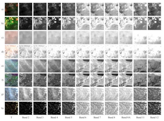
Figure 1.
Four different scenes. Rows (a,c,e,g) are cloud contaminated images; rows (b,d,f,h) are corresponding cloud-free images. All bands are resized to the same size for better presentation.
In this paper, we propose a deep learning-based network to handle thin cloud removal in Sentinel-2A images. The network is mainly designed to fuse spectral information of SWIR bands and Vis/NIR bands to better remove thin clouds in Vis/NIR bands. We also take the vegetation red edge (VRE) bands into consideration, because these bands are also less influenced by thin clouds than visible bands. The experiment is conducted both on real and simulated paired cloud and cloud-free dataset covering the globe.
1.2. Related Works
The removal of thick clouds usually requires multitemporal images from the same location [11,12,13]. In Tseng et al. [14], cloud pixels were directly replaced with clear pixels. Zhang and Wen [15] proposed a discriminative robust principal component analysis (DRPCA) algorithm to recover the background information under thick clouds. Sparse reconstruction was used for cloud removal with time series remote sensing images in Cerra et al. [16]. Image patches clone was adopted to restore background under cloud regions in Lin and Tsai [17]. Chen et al. [18] proposed a spatially and temporally weighted regression model to reconstruct ground pixels occulted by clouds. A nonnegative matrix factorization and error correction algorithm (S-NMF-EC) was proposed in Li and Wang [19] to fuse auxiliary HR and low resolution (LR) cloud-free images to obtain cloud-free HR images. Although thick clouds can be removed by these methods, multitemporal data is required to reconstruct the signal blocked by thick clouds.
The transmittance of clouds increases as thickness of thin clouds decreases [10]. Once the clouds are thin enough, the background signal can transmit through thin clouds and be received by optical satellite sensors, which makes it possible to reconstruct the background signal. Thus, thin clouds removal usually relies on a single cloudy image. Since the response to clouds varies with the wavelength, the features of multispectral bands are very beneficial for the correction of cloud contaminated images. Based on statistics collected on many remote sensing images, the haze optimized transformation (HOT) assumed that ground reflectance in blue and red bands is linearly correlated under clear conditions [20]. An iterative HOT (IHOT) method was proposed in Chen et al. [21] to detect and remove thin clouds in Landsat imagery. Cloudy and corresponding clear images were used in IHOT to solve the spectral confusion between clouds and bright surfaces. Xu et al. [22] proposed a signal transmission and spectral mixture analysis (ST-SMA) algorithm in which the cloud removal model considered the transmission and absorption of clouds. The spectral-based methods can make use of spectral information to remove thin clouds, but they do not take the spatial correlation of neighborhood pixels into consideration. Some other methods for thin cloud removal rely on filtering the cloud component in frequency domain.
There are many methods based on physical model and filtering for cloud/haze removal. In the homomorphic filtering (HF) method [23], Fourier transform was used to separate thin cloud and background components, then a linear filter was adopted to remove the cloud component. Shen et al. [24] proposed an adaptive HF (AHF) method improving HF by treating each spectral band differently and using cloud masks to keep cloud-free areas unchanged. A max–min radiation correction was applied to the result of fast Fourier transform (FFT) and low-pass filter on each band in Liu and Wang [25] to eliminate the influence of transmission and enhance contrast. The methods based on homomorphic filtering can remove cloud components, but low frequency components in the background signal are also removed. Based on the analysis of human visual system, Retinex [26] was proposed to solve the illumination imbalance in images. It was improved in Jonson and Rahman [27], who adopted Gaussian filtering to estimate the incident light. Multi-scale Gaussian filtering in Retinex (MSR) has been proved to be efficient in handling color rendition and dynamic range compression [28]. In order to adjust the color distortion caused by the enhanced contrast in local areas of the image, a color recovery factor was added to MSR (MSRCR) in Jonson and Rahman [29]. MSRCR has been adopted as official image processing tool by NASA and widely used for image dehazing. Although Retinex-based methods can restore some information in images, the incident light estimated by Gaussian filtering is far from the real incident light.
Deep learning (DL) methods have developed rapidly in recent years due to the great improvement of computing performance and increased availability of labelled data. Convolutional neural network (CNN) is the most effective and widely used in image processing and computer vision fields. CNN has been applied to image classification [30], semantic segmentation [31], image generation [32], and image restoration [33]. Most of these tasks were further improved by adopting Resnet [34] and U-Net [35] architectures. The residual architecture was originally designed to solve the problem of information loss in the training of deep CNN by adding input to output and has been widely used for image segmentation recently. The U-Net architecture introduced skip connection that connects down-sampling and symmetrical up-sampling layers to make full use of the features at low and high levels. Differently from Resnet, skip connections in U-Net concatenate the feature maps of convolution and corresponding deconvolution at feature channel, which is more effective than Resnet in using multi-layer features. Many DL-based methods have been proposed to improve the capacity of automatic data processing and solve the technical problems in the remote sensing field. CNN is widely used for remote sensing image processing [36,37], such as land use and land cover classification [38,39], hyperspectral image classification [40,41,42], remotely sensed scene classification [43,44], object detection [45,46], and image synthesis [47].
Due to the good performance of CNN in image inpainting, many CNN-based methods have been successfully applied to thick cloud removal in remote sensing images. Li et al. [48] designed a convolutional–mapping–deconvolutional (CMD) network in which optical and SAR images in the same region were transferred into target cloud-free images. Then the cloud pixels in cloudy images were replaced by corresponding cloud-free pixels from the target cloud-free images. In Meraner et al. [49], a DSen2-CR was proposed to fuse SAR image and optical images to remove thick cloud in Sentinel-2 images. DSen2-CR concatenated SAR image and Sentinel-2 image at spectral channel as input and learned the residual between a cloud image and the corresponding cloud-free image. Generative adversarial networks (GANs) were also adopted for thick cloud removal by fusing optical and SAR images in Gao et al. [50]. GANs were also used for thin/thick cloud removal with paired cloudy and cloud-free optical remote sensing images from the same region [51]. Such thick cloud removal methods can achieve good results but require corresponding auxiliary data such as synthetic aperture radar (SAR) images, which are not influenced by cloud coverage. In addition, cloud detection [52,53,54,55] and image registration [56] are the necessary steps and important influencing factors for these methods.
Differently from image inpainting, image dehazing aims to remove haze and restore the background information in a single image. The atmospheric degradation model has been widely used in image dehazing. Multi-scale parallel convolution has been proven very useful for producing a transmission map, which is then put into the atmospheric degradation model to get a dehazed image [57]. In Zhang and Patel [58], a densely-connected encoder–decoder and U-Net were used to estimate the transmission map and atmospheric light, respectively. The estimated atmospheric light improved the quality of dehazed image a lot. Although these methods can remove haze in images, the atmospheric degradation model is an empirical model, which cannot accurately simulate the interaction between light and the atmosphere. Therefore, many methods have been recently proposed to directly restore a clear image from a hazy image. In Ren et al. [59], the haze image was driven into three transformed images to handle the influences of atmosphere light, scattering, and attenuation. The model used multi-scale reconstruction losses to learn more details. In Chen et al. [60], the smooth dilated convolution was used to solve the grid artifacts. Differently from previous work, the method designed a gate fusion sub-network to learn the weights of different level features, which were then used for the weight sum of these features. Learning the mapping from hazy image to clear image is very effective, but such methods need paired hazy and clear images, which are challenging to obtain.
Thin clouds in remote sensing images are similar to haze in natural images. Thin clouds let part of the background signal transmit, which makes it possible to restore background information using only cloud-contaminated pixels. Qin et al. [61] designed a multi-scale CNN to remove thin clouds in multispectral images. Instead of merging all bands into one network, individual networks were designed for each band. Then the outputs of each individual network were fused by a multi-scale feature fusion layer. A residual symmetrical concatenation network (RSC-Net) was proposed in Li et al. [62], which took advantage of residual error between cloudy and corresponding cloud-free images to train the cloud removal model. Down-sampling and up-sampling operations that are thought to damage the information in the cloud-free regions were not used in RSC-Net. Cycle-GAN [63] has proven very effective for unpaired image-to-image translation. Inspired by Cycle-GAN, a cloud removal GAN (Cloud-GAN) that transfers a thin cloud image into a cloud-free image was proposed in Singh and Komodakis [64]. Sun et al. [65] proposed a cloud-aware generative network (CAGN) in which convolutional long short-term memory (LSTM) and auto-encoder were combined to detect and remove clouds. The attention mechanism [66] was introduced into CAGN to process cloudy regions differently according to the thickness of clouds. In Li et al. [67], a modified physical model was combined with GANs to remove thin cloud with unpaired images. While producing the clear image, the method also learned the transmission, absorption, and reflection maps from the cloud image. Although these methods have good performances, they only handle bands at a same spatial resolution. This discourages their application to satellite sensors that have multi-spatial resolution bands, especially sensors that have low spatial resolution short wave infrared bands.
Although many deep learning-based methods have been proposed for cloud removal in high spatial resolution remote sensing images and achieved the state-of-the-art performance, most of them only handle the Vis/NIR bands at high spatial resolution and either ignore short wave infrared bands at low spatial resolution that are much less influenced by thin cloud than Vis/NIR bands [64], or rescale low resolution bands to high resolution and then process them with Vis/NIR bands together [49]. Rescaling low resolution bands into high resolution by a manually designed rescaling algorithm can help solve the problem of different spatial resolutions. However, the parameters of the manually designed rescaling algorithm are not optimal, and spectral/spatial information may be lost during the manually designed rescaling process. Convolutional neural networks, which can learn optimal sampling parameters during model training, have been widely used for up/down-sampling features automatically [32,35,68]. Therefore, in order to better preserve/extract the spectral information in low resolution bands, we adopted convolutional layers to handle multi-spectral bands at different spatial resolutions.
There are several high spatial resolution satellites such as Sentinel-2A/B, CBERS-04, ZY-1 02D, and HJ-1B that include low spatial resolution SWIR bands, which makes it desirable to take SWIR bands into consideration when removing thin cloud in Vis/NIR bands. In this paper, we aim to remove thin cloud in Sentinel-2A images, which include four vegetation red edge bands that are also less influenced by thin cloud than visible bands, and propose an end-to-end method based on deep-learning for thin cloud and cloud shadow removal by taking vegetation red edge (VRE) and SWIR bands in Sentinel-2A images into consideration. The main contributions are as follows:
- We propose an end-to-end network architecture for cloud and cloud shadow removal that is tailored for Sentinel-2A images with the fusion of visible, NIR, VRE, and SWIR bands. The spectral features in VRE/SWIR bands are fully used to recover the cloud contaminated background information in Vis/NIR bands. Convolutional layers were adopted to replace manually designed rescaling algorithm to better preserve and extract spectral information in low resolution VRE/SWIR bands.
- The experimental data are from different regions of the world. The types of land cover are rich and the acquisition dates of the experimental data cover a long time period (from 2015 to 2019) and all seasons. Experiments on both real and simulated testing datasets are conducted to analyze the performance of the proposed CR-MSS in different aspects.
- Three DL-based methods and two traditional methods are compared with CR-MSS. The performance of CR-MSS with/without VRE and SWIR bands as input and output is analyzed. The results show that CR-MSS is very efficient and robust for thin cloud and cloud shadow removal, and it performs the better when taking VRE and SWIR bands into consideration.
2. Materials and Methods
2.1. Sentinel-2A Multispectral Data
To validate the performance of CR-MSS, Sentinel-2A imagery is selected as the experimental data. Sentinel-2A is a high-resolution multi-spectral imaging satellite that carries a multi-spectral imager (MSI) covering 13 spectral bands in the visible, near infrared, and shortwave infrared (Table 1). The wavelengths of Sentinel-2A image range from 0.443 µm to 2.190 µm and contain four bands in the vegetation red-edge, which is effective for monitoring vegetation health information. Band 1 is used to detect the Coastal aerosol, and bands 9/10 are used to monitor the water vapour/Cirrus, respectively. These bands are used for detecting and correcting the atmospheric effects rather than observing the land surface [49], which means that the atmosphere information in these bands are the most used for practical applications. In Meraner et al. [49], the cloud removal results were worst on 60 m bands even with SAR image as auxiliary input, and atmosphere conditions differ a lot in one day in the same area, let alone in 10 days. Therefore, the introduction of these 60 m bands is not necessary and would not be beneficial to cloud removal in other bands. Therefore, bands 1/9/10 were discarded in our experiments; only bands 2/3/4/8 (Vis/NIR) with size = 10,980 × 10,980 pixels and 5/6/7/8A/11/12 (VRE/SWIR) with size pixels in Sentinel-2A Level-1C product were selected in our experiments.

Table 1.
Sentinel-2A sensor bands. Bands used in our study are marked in bold.
2.2. Selection of Training and Testing Data
In the cited related non-deep learning-based works, the methods are usually empirically based and directly tested on experimental data, e.g., seven Landsat TM images covering 12 different land cover types in Canada were used to test the performance of HOT [20] on cloud removal. In IHOT [21], the method was tested on four pairs of cloudy and cloud-free Landsat, eight images from cropland, urban, snow, and desert land covers. Shen et al. [24] employed five Landsat ETM+ and two GaoFen-1 cloudy images as testing data in AHF. However, in the cited related deep learning-based works, training data is necessary, e.g., eight pairs and two pairs of Landsat, eight images, were selected for training and testing, respectively, in RSC-Net [62]. Singh and Komodakis [64] chose 20 cloudy and 13 cloud-free images to train Cloud-GAN and tested the performance on five synthetic scenes. In Li et al. [67], 16 training sites and four testing sites were chosen in the East coast of United States. The ratio between training and testing images most of these deep learning-based cloud removal methods was 80/20%.
In these related works, the spatial coverage of the study areas only ranges from cities to countries, the datasets are relatively small, and the time period between cloud and corresponding cloud-free images are usually longer than half a month, which means land cover may change greatly. The datasets in non-deep learning-based methods are mainly used for testing, and thus cannot be employed to train deep learning-based methods. Although the experimental data in cited deep learning-based methods includes training and testing data, those datasets were relatively small and were not stratified by land cover types; therefore, those study areas lack diversity.
In this study, cloudy and corresponding cloud-free images from Sentinel-2A satellite are used to train and test all methods. In order to better evaluate the effectiveness of CR-MSS over large scale regions and different land cover types, the training and testing areas are evenly distributed worldwide and according to three main land covers: urban, vegetation, and bare land. Figure 2 shows the 36 locations from all over the world selected as study areas. For training, we chose 28 areas all over the globe including 10 urban areas, 10 vegetation areas, and eight bare land areas. Eight areas were chosen all over the globe for testing, including three urban areas, three vegetation areas, and two bare land areas. Therefore, there is one testing area for three to four training areas, depending on the land cover. From Figure 2, it also can be seen that each testing site is surrounded by three to four training sites. The total ratio between training and testing images in our experiment is 77.8%/22.2%, i.e., slightly more testing data in proportion than the related deep-learning works. The details of 36 pairs cloud and corresponding cloud-free images are shown in Table 2.
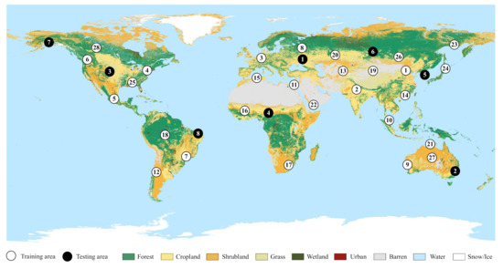
Figure 2.
Distributions of training and testing data. Training areas are marked in white; testing areas are marked in black. The number in each area is corresponding to each number in Table 2. The landcover background is derived from ESA-CCI-LC [69].
Table 2.
Details of Sentinel-2 training and testing image pairs.
We set the time lag of the acquisition dates of cloudy and corresponding cloud-free images to 10 days, which is the revisit time of Sentinel-2A satellite, to minimize the difference between cloudy and cloud-free images as much as possible. The manual collection of one single pair of cloudy and corresponding cloud-free images with the shortest time lag of data acquisition took about 30 min, because many Sentinel-2A images are covered with clouds, and it was challenging to find a corresponding cloud-free image. To assess the performance of CR-MSS for cloud removal in different seasons, the acquisition dates of training and testing data were from 2015 to 2019, in which all seasons are covered. Twenty-eight training image pairs and eight testing image pairs were collected from the Copernicus Open Access Hub website, under the conditions: (1) widely distributed, (2) covering all seasons, and (3) shortest time lag for data collection. The performance of all methods can be fully evaluated with the all these training and testing data, which have the shortest time lag and different land cover types and covers all seasons. The dataset is shared on https://github.com/Neooolee/WHUS2-CR.
2.3. Method
In the proposed CR-MSS method, the paired cloudy and cloud-free multispectral images are used in end-to-end training. Inspired by U-Net architecture, CR-MSS is designed to make better use of the features at different levels. CR-MSS has two input/output branches that are used to handle Vis/NIR bands and VRE/SWIR, respectively. The features of multispectral images are first fused after processed by input branches and then compressed before output branches. The network architecture of CR-MSS is introduced in this section.
We group Vis/NIR bands and VRE/SWIR into two separate multispectral images, that are then inputted to two input branches in CR-MSS. Pooling is the most common operation for down-sampling the feature maps in deep learning, as the cost of losing neighborhood information by this operation. Instead, we use convolutional layers with stride = 2 instead of the pooling layers to down-sample the feature maps in CR-MSS. Convolutional layer can preserve neighborhood information as much as possible by optimizing the parameters. The deconvolution layer with stride = 2 is adopted to up-sample the feature maps. The kernel sizes of convolutional and deconvolution layers in CR-MSS are set to and , respectively. The details of the convolutional and deconvolution layers are as follows:
- The convolution layer contains multiple convolution kernels and is used to extract features from input data. Each element that constitutes the convolution kernel corresponds to a weight coefficient and a bias. Each neuron in the convolution layer is connected with multiple neurons in the adjacent region from the previous layer, and the size of the region depends on the size of the convolution kernel.
- The deconvolution layer is used to up-sample the input data, by interpolating between the elements of the input matrix, and then, constructing the same connection and operation as a normal convolutional layer, except that it starts from the opposite direction.
As shown in Figure 3, there are two input branches in CR-MSS: Vis/NIR input branch (Vis/NIR-In) and VRE/SWIR input branch (VRE/SWIR-In). A fusion tunnel performs feature fusion, while the compression tunnel performs feature compression. Vis/NIR-In is for processing Vis/NIR bands; VRE/SWIR-In is for VRE/SWIR bands. To extract low-level features of the input images and preserve the original information from input images, the stride in the first convolutional layer in each input branch is set to 1 to keep the size of inputs unchanged. Since Vis/NIR has higher spatial resolution than VRE/SWIR, Vis/NIR-In has one more convolution layer than VRE/SWIR-In, with stride = 2. This extra convolutional layer in Vis/NIR-In is used to down-sample the input feature maps to the same size as the output of VRE/SWIR-In.
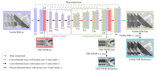
Figure 3.
The architecture of CR-MSS. The number under/on each block is the number of feature maps of it. The feature maps in each dotted box are concatenated at feature channels.
As we know, there is a strong correlation among the spectral responses of the same target in different bands. Since SWIR bands are the least affected by clouds among all bands, and VRE bands are less affected than Visible bands, the spectral features of VRE/SWIR bands can be used to restore the missing information in Visible bands. Therefore, the output feature maps of VRE/SWIR-In are concatenated with the output feature maps of Vis/NIR-In at feature (spectral) channel. Then the concatenated feature maps are put into the fusion tunnel to fuse the features from all experimental bands. There are four convolutional layers in the fusion tunnel. The stride of each convolutional layer is set to 2 to down-sample the feature maps and extract high-level features. It can be seen that the number of concatenated feature maps is 192 (128+64); after being processed by the first convolutional layer in the fusion tunnel, the number of feature maps is extended to 256. In this way, the features in Vis/NIR/VRE/SWIR bands are fused and expanded. The next three convolutional layers in the fusion tunnel are used to fuse and extract more features for the restoration of background information.
There are four deconvolution layers with stride = 2 in the compression tunnel that are used to up-sample the feature maps and compress features. The output feature maps of the last convolutional layer in the fusion tunnel are put into the first deconvolutional layer in compression tunnel directly. To make full use of features at different levels and generate high quality cloud-free images, the output of each convolutional layer before the middle convolutional layer is copied and concatenated with the output of each symmetric deconvolution layer. These concatenations can solve the problem of information loss of the original images in the process of down-sample operations and help the network converge faster.
Because there are two input branches to handle Vis/NIR bands and VRE/SWIR bands in CR-MSS, respectively, the CR-MSS also has two output branches to handle Vis/NIR and VRE/SWIR bands. The output branches and the input branches are symmetric in CR-MSS. The output branch that handles Vis/NIR bands (Vis/NIR-Out) has one more deconvolution layer than the branch that handles VRE/SWIR bands (VRE/SWIR-Out). This deconvolution layer in Vis/NIR-Out is used to up-sample the feature maps to the same size as the input of Vis/NIR-In. In order to get the same number of channels as in input images, we add a convolutional layer with stride = 1 and output channels (bands) = 4 and 6 in Vis/NIR-Out and VRE/SWIR-Out branches, respectively. In this way, Vis/NIR-Out outputs a multispectral image with Vis/NIR bands; VRE/SWIR-Out outputs a multispectral image with VRE/SWIR bands.
We adopt L1 loss as the loss function of CR-MSS. For each band in input images, we measure the difference between the output cloud-free and corresponding ground-truth or reference cloud-free band to optimize CR-MSS. The average loss over all bands is taken as the final loss. The parameters of CR-MSS are updated with the loss function as follows:
where z is the input image, the ith band in reference images, the ith band in generated cloud-free images, and k the total number of spectral bands of z. CR-MSS will learn the difference between and x, then optimize the parameters to generate more clear images. After CR-MSS is well-trained, it can restore thin cloud images into cloud-free images.
2.4. Data Pre-Processing and Experiment Setting
Three DL-based methods and two traditional methods for cloud removal are compared with CR-MSS in our experiments: RSC-Net [62], U-Net [35], Cloud-GAN [64], AHF [24], and MSRCP [70]. Because CR-MSS is designed for cloud removal in a single image, multi-temporal cloud removal methods are not included in this comparison. RSC-Net and U-Net are end-to-end methods that require paired cloudy and corresponding cloud-free images. Cloud-GAN is a semi-supervised method that requires unpaired cloudy and cloud-free images. AHF is an adaptive homomorphic filtering method for cloud removal and requires cloud masks. MSRCP is based on MRSCR and with cuda parallel acceleration for image enhancement such as image dehazing.
In order to train the CNN-based methods, we cropped all experimental images into small patches without overlapping by slide windows of different sizes. Since the spatial resolution of Vis/NIR bands and VRE/SWIR bands is 10 and 20 m, respectively, we set the corresponding slide window sizes to and pixels. The area extents of each patch at 10 m resolution matches that of each corresponding patch at 20 m resolution. In this way, 17,182 pairs of cloudy and corresponding cloud-free multispectral images are produced. Additionally, 13,389 pairs of training samples are generated from 28 pairs of training images, and 3782 pairs of testing samples are generated from eight pairs of testing images. The training dataset was augmented by flipping training samples horizontally and vertically, and rotating them at 90°, 180°, and 270° angles. In this way, 80,334 pairs of cloudy and cloud-free training patches were obtained. The traditional methods can process the whole image at once to perform cloud removal. Because the AHF method requires cloud masks, we adopt the official Sentinel-2 cloud masks tool Sen2Cor [71] for Sentinel-2 to produce the cloud masks in our experiment.
Because the spectral reflectance values of objects in images will change in 10 days, the cloud-free images in testing data cannot be used to quantitatively evaluate the performance of all methods on spectral information preservation. There are many methods using simulated cloud images to evaluate their performances [12,50,72,73]. Therefore, in order to quantitatively evaluate the performances of all methods on spectral information preservation, we simulated cloudy images with Adobe Photoshop following [65], from cloud-free images of the testing dataset. First, we added a transparent layer for each band with different transparency rate, then we applied the Photoshop command Filter -> Render -> Cloud on each transparent layer to produce a cloud layer. Finally, each transparent and band pair were fused together to obtain a cloud band. All methods were applied on the simulated cloud images, in order to remove clouds and quantitatively evaluate the performances of all methods on spectral information preservation.
In the training stage, all deep learning-based methods were trained on real cloud and cloud-free image pairs in training dataset listed in Table 2. In the testing stage, all baseline methods and CR-MSS were tested on real cloud and cloud-free image pairs for PSNR and SSIM values, and on simulated cloud and cloud-free image pairs for NRMSE value, to better control for spectral reflectance changes, as explained in the previous paragraph. Figure 4, Figure 5, Figure 6, Figure 7, Figure 8, Figure 9, Figure 10, Figure 11, Figure 12 and Figure 13 show the cloud removal results of all methods on real cloud and cloud-free images.
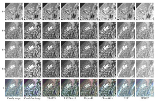
Figure 4.
Visual comparison results on urban sample (Ukraine) under thin clouds from first real testing image pair in Table 2. T, B2, B3, B4, and B8 are true color composited image, bands 2, 3, 4, and 8, respectively. Columns 1–8 are cloudy and corresponding cloud-free images, results of CR-MSS, RSC-Net-10, U-Net-10 and Cloud-GAN, AHF, and MSRCP.
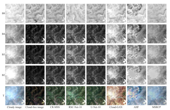
Figure 5.
Visual comparison results on vegetation sample (Australia) under thin clouds from second real testing image pair in Table 2. T, B2, B3, B4, and B8 are true color composited image, bands 2, 3, 4, and 8, respectively. Columns 1–8 are cloudy and corresponding cloud-free images, results of CR-MSS, RSC-Net-10, U-Net-10 and Cloud-GAN, AHF, and MSRCP.
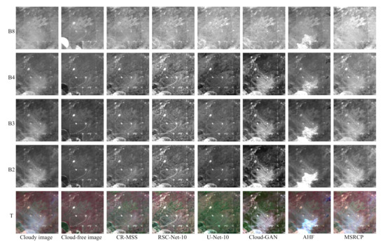
Figure 6.
Visual comparison results on bare land sample (United States) under thin clouds from third real testing image pair in Table 2. T, B2, B3, B4, and B8 are true color composited image, bands 2, 3, 4, and 8, respectively. Columns 1–8 are cloudy and corresponding cloud-free images, results of CR-MSS, RSC-Net-10, U-Net-10 and Cloud-GAN, AHF, and MSRCP.
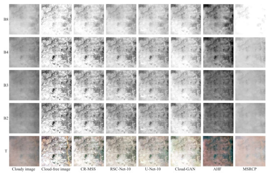
Figure 7.
Visual comparison results on bare land sample (Nigeria) under thin clouds from 4th real Table 2. T, B2, B3, B4, and B8 are true color composited image, bands 2, 3, 4, and 8, respectively. Columns 1–8 are cloudy and corresponding cloud-free images, results of CR-MSS, RSC-Net-10, U-Net-10 and Cloud-GAN, AHF, and MSRCP.
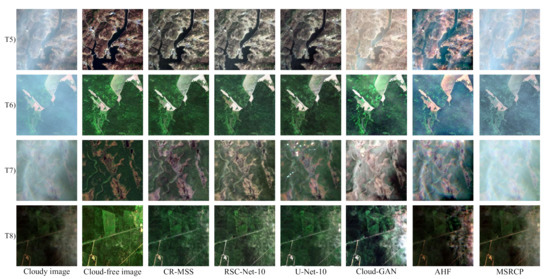
Figure 8.
Visual comparison on four samples. (T5), (T6), (T7) and (T8) are true color composites from fifth, sixth, seventh, and eighth real testing image pairs in Table 2. Columns 1–8 are cloudy and corresponding cloud-free images, results of CR-MSS, RSC-Net-10, U-Net-10 and Cloud-GAN, AHF, and MSRCP.
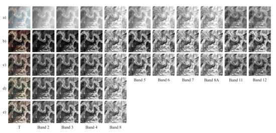
Figure 9.
Visual comparison results on mountain sample (South Korea) under thin clouds from fifth real testing image pair in Table 2. By row: (a) cloudy image, (b) corresponding cloud-free image, (c) results of CR-MSS, (d) CR-MSS-10-4, and (e) CR-MSS-4-4.
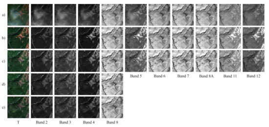
Figure 10.
Visual comparison results on grass sample (Russia) under thin clouds from sixth real testing image pair in Table 2. By row: (a) cloudy image, (b) corresponding cloud-free image, (c) results of CR-MSS, (d) CR-MSS-10-4, and (e) CR-MSS-4-4.
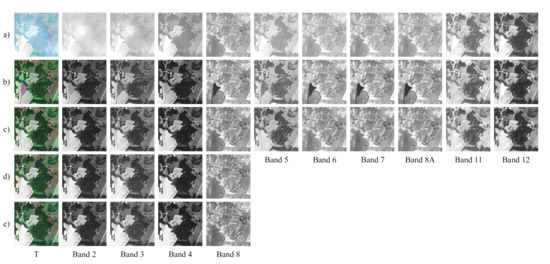
Figure 11.
Visual comparison results on forest sample (United States) under thin clouds from seventh real testing image pair in Table 2. By row: (a) cloudy image, (b) corresponding cloud-free image, (c) results of CR-MSS, (d) CR-MSS-10-4, and (e) CR-MSS-4-4.
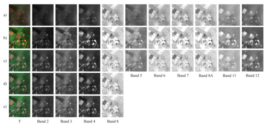
Figure 12.
Visual comparison results on farmland sample (Brazil) under thin clouds and cloud shadows from eighth real testing image pair in Table 2. By row: (a) cloudy image, (b) corresponding cloud-free image, (c) results of CR-MSS, (d) CR-MSS-10-4, and (e) CR-MSS-4-4.
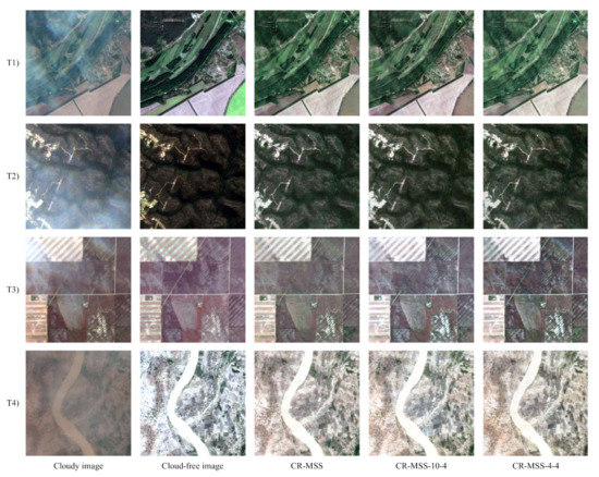
Figure 13.
Visual comparison on four samples. (T1), (T2), (T3), and (T4) are true colour composites from first, second, third, and fourth real testing image pairs in Table 2. Columns 1–5 are cloudy and corresponding cloud-free images, results of CR-MSS, RSC-Net-10, U-Net-10, and Cloud-GAN.
The inputs of AHF, MRSCR, and Cloud-GAN are Vis/NIR bands. Since CR-MSS is designed to handle Vis/NIR and VRE/SWIR bands together, the input of CR-MSS is Vis/NIR/VRE/SWIR bands. Because RSC-Net and U-Net are end-to-end deep learning-based methods similar to CR-MSS, in order to compare RSC-Net and U-Net with CR-MSS fairly, VRE/SWIR bands were first rescaled to 10 m resolution by bi-linear interpolation, then concatenated with Vis/NIR bands to train RSC-Net-10 and U-Net-10. In addition, to analyze the influence of the VRE/SWIR bands on CR-MSS performance for thin cloud removal, we conducted ablation experiments, i.e., with or without VRE/SWIR bands as inputs/outputs or not.
The hyper-parameters are set the same for all deep learning-based methods. The batch size is set to 1, and iterations for training are set to 600000. Adam-optimizer [74] is adopted to optimize the parameters of all networks, and the hyper parameters of Adam-optimizer are fixed as: , , and the initial learning rate = 0.0002, with exponential decay at decay rate = 0.96. The training and testing experiments are both conducted with the TensorFlow running on Windows 7 operating system on a 16 Intel (R) Xeon CPU E5-2620 v4 @ 2.10 GHz and an NVIDIA GeForce GTX 1080Ti with 11 GB memory.
We take peak signal to noise ratio (PSNR), structural similarity index measurement (SSIM), and normalized root mean square error (NRMSE) as the quantitative evaluation measures. The PSNR and SSIM values of one single testing sample and average of all testing samples in each band are calculated to better compare the performances of all methods. As in Meraner et at. [49], the average NRMSE values in each band over all simulated testing samples were calculated to analyze the spectral preservation in each band.
3. Results
3.1. Comparison of Different Methods
To better present the cloud removal results of different areas worldwide, we selected one sample pair from each testing area. The experimental results of all cloud removal methods on these selected samples are presented in Figure 4, Figure 5, Figure 6, Figure 7 and Figure 8. Figure 4, Figure 5, Figure 6 and Figure 7 show the cloud removal results on each band of four samples from the first, second, third, and fourth testing pairs, respectively. The inputs/outputs were original Vis/NIR/VRE/SWIR bands for CR-MSS, original Vis/NIR, and rescaled VRE/SWIR bands for RSC-Net-10 and U-Net-10, and Vis/NIR bands for other baseline methods. Figure 4, Figure 5, Figure 6 and Figure 7 show results of CR-MSS and baseline methods with Vis/NIR bands.
We can see that the results of CR-MSS are visually better than all compared methods on all bands in these Figs. For example, in Figure 5, the impact of cloud is very severe on background signal. CR-MSS removes most clouds in Vis/NIR bands. While results of RSC-Net-10 and U-Net-10 contain much noise in cloudy regions, Cloud-GAN translates the input cloudy image into another cloud contaminated image, the style of which is completely different from the input cloudy image and makes the result even worse. This is caused by the influence of cycle-consistent of Cloud-GAN. In the training of Cloud-GAN, it first translates a cloudy image into a cloud-free image. Then, the translated cloud-free image is translated back into the input cloudy image, which makes the textures of the cloud-free image and input cloudy image consistent. This results in some cloud information being retained in the translated cloud-free image. Results of both AHF and MSRCP on Figure 5, Figure 6 and Figure 7 are not good visually, because the cloud component cannot be completely filtered out by Homomorphic filtering in AHF, and the model in MSRCP does not take the reflection of cloud into consideration. However on Figure 7, AHF have a better visual result than MSRCP because the thin clouds are fairly uniform and can be removed by low-pass filtering.
Figure 8 shows the true color composited results of four samples in fifth, sixth, seventh, and eighth testing pairs. Visually, the results of CR-MSS seem more realistic than baseline methods, and MSRCP looked the worst among all methods, while Cloud-GAN performs the worst among all deep learning-based methods. It is worth noticing that the (T8) in Figure 8 contains thick clouds and cloud shadows, and CR-MSS removes cloud shadows and most of the clouds, but results of all baseline methods still include many clouds.
Table 3 and Table 4 show the corresponding PSNR and SSIM values of samples in Figure 4, Figure 5, Figure 6, Figure 7 and Figure 8, respectively. It can be seen that CR-MSS obtains the best performance on PSNR and SSIM values in most cases. It is worth noticing that AHF performs best on SSIM values on Figure 6 at bands 4/8 and T8 in Figure 8 at band 8. Although the visual results of AHF on Figure 6 and T8 in Figure 9 are worse than CR-MSS, AHF usea cloud masks to preserve the cloud-free regions, which improves the SSIM values on average.
Table 5 shows the averaged PSNR and SSIM values on each band over all testing samples. It can be seen that CR-MSS outperforms the compared methods on SSIM values in all bands as well as PSNR values in bands 3/8, and performs almost the same as the best methods on PSNR in bands 2/4 (U-Net-10 and RSC-Net-10, respectively). The SSIM values illustrate that CR-MSS can preserve more structure information than compared methods. Since both U-Net-10 and RSC-Net-10 are end-to-end methods, they achieve good results that are close to the results of CR-MSS. Still, CR-MSS has the advantage of being able to restore background information in all bands, not just Vis/NIR bands.
Table 5.
Average PSNR and SSIM values of all methods over all eight real testing image pairs from Table 2 (3782 testing samples). Best results are marked in bold.
U-Net-10 extracts the features at different levels by max/average pooling and combining these features with skip connections. The different level features are fully used by the skip connection, but the neighborhood pixel information is altered in the pooling operation. This is probably the reason why U-Net-10 results are worse than CR-MSS. RSC-Net-10 uses symmetrical concatenations to preserve the information in cloud-free regions. Since it does not down-sample the feature maps, the receptive field of RSC-Net-10 is very small, which means the information from long distance neighborhood pixels cannot be used to restore background information. Unlike U-Net-10 and RSC-Net-10, CR-MSS down-samples the feature maps by convolutional layers with stride = 2, thus preserving neighborhood pixel information and keeping a large receptive field. Although Cloud-GAN does not need paired cloud and cloud-free images, which are very time-saving for the generation of training dataset, Cloud-GAN performs the worst on SSIM value among all methods. This may be because it not only translates a cloudy image into a cloud-free image, but also preserves some texture features from the cloudy image that are used to restore the translated cloud-free image back to a cloudy image—and by this operation, the retained texture features include cloudy texture features, or the training of the generators, ending in a poor location of the optimization landscape. The instability of training adversarial networks also makes it difficult to generate realistic cloud-free images. AHF can filter some cloud components, but the low frequency components in background may be filtered out as well. MSRCP estimates the incident light by Gaussian filtering, which can help to reduce the influence of light but will not help much to remove thin clouds. This is the reason why AHF performs better than MSRCP in most cases on thin cloud removal. Because clouds have the least effects in SWIR bands, and VRE bands are less influenced by clouds than VIS bands, more background information is contained in these bands. By taking VRE/SWIR bands into consideration, CR-MSS can restore more information in Vis/NIR bands. This is another reason why CR-MSS can always obtain better performance on SSIM than compared methods.
Table 6 shows the computing time for all methods. The deep learning base methods are much more efficient than traditional methods. MSRCP takes the longest time, because the Gaussian filtering is very time-consuming, especially in such large images as Sentinel-2. RSC-Net-10 was the fastest method, only outputting 32 feature maps in each convolutional and deconvolutional layer, which reduces a lot of calculations. Although CR-MSS had a longer computing time than compared deep learning-based methods, the difference is marginal, and CR-MSS obtained the best performance among all methods in most cases.
Table 6.
Computing time of different cloud removal methods (in minutes and seconds on a Sentinel-2 image with size 10,980 10,980 pixels. Best results are marked in bold.
3.2. Influence of the Temporal Shift between Images
As mentioned in Section 2.2, the temporal shift between paired cloud and cloud-free images is 10 days in all experimental data. Table 7 shows the averaged PSNR and SSIM values of all methods on testing samples of different land covers. The highest values are marked in bold, and the symbol ‘/’ is used to represent the band that is not included in the training and testing. We can see that CR-MSS performs the best for SSIM values on urban areas, vegetation areas, and bare land on bands 2/3/4/8, except on band 2 for vegetation, which is slightly better for RSC-Net-10. It can be seen that on vegetation areas, CR-MSS has five PSNR and three SSIM values that are lower than those of RSC-Net-10 or U-Net-10, while only 2 PSNR and 1 SSIM values are lower on Urban areas and four PSNR and one SSIM values are lower on bare land. This is because during the same temporal shift of 10 days between training and testing images, the spectral information in Vis/NIR/VRE/SWIR bands over vegetation areas changes faster than over the two other land cover areas. With VRE/SWIR bands as output, the reference images change more in CR-MSS than baseline methods that only process Vis/NIR bands. Therefore, the temporal shift on vegetation areas influence the performance of CR-MSS more than baseline methods. However, it is worth noticing that CR-MSS obtains competitive SSIM values on vegetation areas, because SSIM contains the properties of the object structure that will not change much in vegetation areas within a short temporal shift. It can also be seen that CR-MSS obtains the best performance on SSIM values on urban and bare land areas on nine out of 10 bands, because the influences of temporal shift on the properties of the object structure are much less than on vegetation areas in the same temporalhift.
Table 7.
Average PSNR and SSIM values over different land covers and all eight real testing image pairs from Table 2 (3782 testing samples). Best results are marked in bold.
3.3. Influence of VRE/SWIR Bands
To analyze the influence of the VRE/SWIR bands, we conducted two other experiments with or without VRE/SWIR bands as inputs, and without VRE/SWIR bands as outputs. The experiment with Vis/NIR/VRE/SWIR bands as inputs and Vis/NIR bands as outputs is called CR-MSS-10-4. The experiment with Vis/NIR bands as inputs and outputs is called CR-MSS-4-4. CR-MSS-10-4 has Vis/NIR-In and VRE/SWIR-In in the input branches, while CR-MSS-4-4 only has Vis/NIR-In branch. Both CR-MSS-10-4 and CR-MSS-4-4 only have Vis/NIR-Out branch.
Figure 9, Figure 10, Figure 11 and Figure 12 show cloud removal results of CR-MSS, CR-MSS-10-4 and CR-MSS-4-4 on four samples from the fifth, sixth, seventh, and eighth real testing pairs. The first and second rows show the cloud contaminated image and the corresponding cloud-free image. The following rows show the results of CR-MSS, CR-MSS-10-4, and CR-MSS-4-4, respectively. It can be seen that results on Vis/NIR bands are quite good visually. However, as shown in Figure 10, the sample (from the sixth testing image pair) contains unevenly distributed clouds. Thus, the cloud effect in this sample is not completely removed by CR-MSS-10-4 and CR-MSS-4-4, while CR-MSS removes clouds in this sample on all experimental bands.
Figure 12 shows a sample (from the eighth testing image pair) affected by cloud shadows. It can be seen that the effect of cloud shadow is removed by CR-MSS, CR-MSS-10-4, and CR-MSS-4-4. The results on other four samples from the first, second, third, and fourth testing pairs are presented in Figure 13. The first two columns are the cloud contaminated image and corresponding cloud-free image. The last three columns are the results of CR-MSS, CR-MSS-10-4, and CR-MSS-4-4. It can be seen that most of the clouds over different land cover types can be removed by all CR-MSS-based methods. It can be seen that CR-MSS-based methods try to restore the original background information in the cloudy image, rather than directly transferring the cloudy image into the reference image 10 days apart from the input cloud image.
Table 8 shows corresponding PSNR and SSIM values of Figure 9, Figure 10, Figure 11 and Figure 12. The average PSNR and SSIM values of real samples in Figure 13 and all 3782 real testing samples are listed in Table 9 and Table 10, respectively. From Table 8, Table 9 and Table 10, we can see that the performances of CR-MSS are better than CR-MSS-10-4 and CR-MSS-4-4 most of the time. However, the PSNR and SSIM values of all CR-MSS-based methods are similar. Although CR-MSS-10-4 has the same input bands as CR-MSS, CR-MSS obtains better results on most bands. This is because the output of CR-MSS contains VRE/SWIR bands, which are not included in the output of CR-MSS-10-4, and the restoration of VRE/SWIR bands can add more supervision information on the training of CR-MSS than the restoration of Vis/NIR bands. CR-MSS-4-4 with only Vis/NIR bands as inputs and outputs performs the worst among all CR-MSS-based methods. This is because a lot of background information is damaged by clouds on visible bands. Although NIR band is less affected by clouds than Vis bands, the information it contains is limited and less than bands 8A/11/12 combined. Thus, CR-MSS and CR-MSS-10-4 obtain slightly better results than CR-MSS-4-4.
Table 9.
Average PSNR and SSIM values of four real samples in Figure 13. Best results are marked in bold.
Table 10.
Average PSNR and SSIM values of CR-MSS-based methods over all eight real testing image pairs from Table 2 (3782 testing samples). Best results are marked in bold.
As the results of different methods and different number of input bands show, CR-MSS can achieve the best performance in these experiments on most bands. SSIM values of CR-MSS on VRE/NIR/SWIR bands are more acceptable than those on visible bands. This means that the cloud effect is less in bands VRE/NIR/SWIR than visible bands, which is the reason why CR-MSS is designed to take multi-spectral images as input. With more input and output bands, CR-MSS can make full use of the spectral information to restore cloud contaminated images.
Comparing results from Table 4 and Table 10, it can be seen how well CR-MSS based methods perform on average over the eight testing image pairs compared to baseline methods when using the same input and output bands. For every Vis/NIR band taken separately, CR-MSS-4-4 has a PSNR slightly lower but close to each best result among the baseline methods. As it comes to SSIM values, CR-MSS-4-4 outperforms every baseline method on every Vis/NIR band. This demonstrates that, even when restricted to visible and NIR bands, the proposed CR-MSS method performs similarly well or better than baseline methods, depending on the measure. One of the main advantages of CR-MSS method remains its capability to handle more than visible and NIR bands seamlessly, as well as the ability to further improve results on visible and NIR bands when adding other bands as inputs.
As can be seen in Figure 4, Figure 5, Figure 6, Figure 7, Figure 8, Figure 9, Figure 10, Figure 11, Figure 12, Figure 13 and Table 3, Table 4, Table 7, and Table 8, all methods perform best on vegetation areas under thin clouds, but worst on urban areas under thin clouds. This is because urban area has more textures than vegetation area, and the details of complex textures in images are very difficult to restore in many image processing tasks.
3.4. Spectral Preservation on Simulated Data
As explained in Section 3.1, we applied all methods to simulated cloud images and then computed NRMSE values between cloud removal results and real cloud-free images. The average NRMSE values in each band over all eight simulated cloud testing samples are shown in Table 11. The best values are marked in bold. The lower the NRMSE value, the more spectral information is preserved. It can be seen that the lowest NRMSE values for bands 3/4/5/6/11/12 fall in CR-MSS based methods, while U-Net-10 performs better for band 2, and RSC-Net performs better for bands 7/8/8A. Cloud-GAN obtains the worst performance on spectral preservation; this may be because Cloud-GAN is a cycle network designed for image style transformation, which preserves more texture information than spectral information.
Table 11.
Average NRMSE values over all eight simulated testing image pairs (3782 simulated testing samples). Best results are marked in bold.
4. Discussion
From the experimental results on the real image dataset, we can see that most of the time, CR-MSS performs the best qualitatively and quantitatively. This is because CR-MSS takes VRE/SWIR bands into consideration when removing cloud in Vis/NIR bands, which is not available in other deep learning-based cloud removal methods in remote sensing images, e.g., Cloud-GAN [64] and CGAN [65] only process RGB bands. Some methods such as Qin et al. [61] and RSC-Net-10 [62] take SWIR bands in Landsat-8 images as input when removing cloud, but it can only handle the images at the same spatial resolution. Although VRE/SWIR bands have lower spatial resolution than Vis/NIR bands in Sentinel-2A images, they are less influenced by cloud than Vis/NIR bands. Similar to super resolution reconstruction, CR-MSS can make full use of the less influenced low spatial resolution VRE/SWIR bands to reconstruct the missing information in much influenced high spatial resolution Vis/NIR bands. Therefore, CR-MSS can also be considered as a combination of cloud removal and super resolution reconstruction.
Experimental results on the simulated dataset show CR-MSS based methods can preserve more spectral information than baseline methods on most bands in simulated cloud images. We understand this simulated cloud dataset is not perfect, and these results should be taken only for their comparative value, not as an indication of how the proposed method would perform on a real dataset. This was just a complementary experiment to quantitatively assess spectral preservation in a way the real cloud dataset could not.
In Meraner et al. [49], Sentinel-2 low spatial resolution bands were first rescaled to 10 m resolution and then processed with Vis/NIR bands and Sentinel-1 SAR images. A hand designed rescaling algorithm was adopted in Meraner et at. [49] to rescale all data to the same resolution. Hand designed rescaling algorithms such as Nearest neighbor, Bilinear, and Cubic convolution have at least one inevitable drawback: the parameters in the algorithms are not optimal for specific tasks. This drawback can be avoided by training the convolution neural network to learn optimal parameters for specific tasks such as cloud removal automatically. Therefore, convolutional layers were adopted to handle multi-spectral bands at different spatial resolution in CR-MSS, and up-sampling low spatial resolution bands to high resolution is not necessary anymore. In addition, up-sampling low spatial resolution bands to high resolution will not produce more useful spatial information when real high resolution bands are already available and introduce more spectral information.
Since single image based cloud removal methods can hardly remove the influence of clouds completely, many multi-temporal based methods have been proposed to solve this problem. Multi-temporal cloud removal methods usually include three steps: first, select a time series images in the same region as the experimental data; then the cloud regions in each image are detected; finally, the cloud-free regions are mosaicked to get a completely cloud-free image. If the spectral information of each cloud-free regions in the mosaicked image are not consistent with each other, radiometric harmonization across the temporal stack will be conducted to solve this problem. Although the components in the mosaicked cloud-free image are completely cloud-free, there are still some limitations to the multi-temporal based methods. (1) Accurate cloud masks are necessary for each image in the multi-temporal stack; those masks are difficult to obtain, especially for thin clouds, and any labelling error compounds across the temporal stack. (2) Time series images used in the methods are acquired at different times, which means the ground information in the mosaicked cloud-free image is not consistent in time. (3) The longest time period of the time series images depends on the revisit time of the satellite and weather conditions: the longer the time period, the less meaningful the result is. (4) Multi-temporal cloud removal methods usually require more input data ad processing than single-image methods. They are naturally justified as part of a whole multi-temporal chain including, e.g., multi-temporal classification or time series analysis. However, if the end application can be achieved with single image (e.g., classification) or dual images (bi-temporal change detection), often single-image cloud removal methods are still preferred in practice for their ease of use.
Although there are many complex and effective deep learning-based networks in the image processing field, U-Net architecture is the most widely adopted in image in-painting, image de-hazing, and image super resolution due to its simplicity and effectiveness. In view of this, CR-MSS adopted U-Net as the main architecture, with some modifications, so that it can be used for handling multispectral satellite images at different spatial resolutions. As a result, CR-MSS remains a relatively simple deep learning model that is easy to understand, implement, and deploy in operational conditions. CR-MSS was designed for thin cloud removal; however, it can also be easily applied to other remote sensing image processing tasks such as cloud detection and semantic segmentation, due to the simplicity and effectivity inherited from U-Net.
5. Conclusions
In this paper, we proposed a thin cloud removal method, CR-MSS, which used the VRE/SWIR spectral information to better restore the original background information contaminated by thin clouds in Vis/NIR bands in Sentinel-2A images. CR-MSS takes Vis/NIR and VRE/SWIR bands of Sentinel-2A images as inputs, grouped into two images at 10 m resolution and 20 m resolution, and fed into separated input/output branches without rescaling low spatial bands to high resolution by hand designed rescaling algorithm. Compared with baseline methods on real and simulated testing datasets, CRMSS can achieve better overall performance for texture and spectral information preservation both qualitatively and quantitatively. Ablation experiments were also conducted to analyze the influence of VRE/SWIR bands on the performance of thin cloud removal in Sentinel-2A images. The experiment results show that even VRE/SWIR bands have lower spatial resolution than Vis/NIR bands; their spectral information can help restore the cloud contaminated pixels in Vis/NIR bands. Additionally, adding VRE/SWIR bands into input and output, CRMSS performs better than only adding VRE/SWIR bands as input. The quantitative results derived from the simulation experiment showed CR-MSS based methods can preserve more spectral information than all baseline methods in bands 2/3/4/8.
In future work, we will improve and apply CR-MSS thin cloud removal to other optical satellites that acquire multispectral images with bands at different spatial resolutions (such as CBERS-04 and ZY-1 02D). We will also modify CR-MSS so that it can be applied to other remote sensing image processing tasks such as cloud detection and semantic segmentation. The combination of generative adversarial networks and CR-MSS will also be taken into consideration to remove clouds in a semi-supervised way.
Author Contributions
Conceptualization: J.L.; methodology: J.L.; visualization: Z.L.; funding acquisition: Z.H.; validation: J.L.; formal analysis: J.L., Z.W., Z.H., and M.M.; supervision: Z.W., M.M., and Z.H.; investigation: Y.W. and Z.L.; writing—original draft preparation: J.L. and Z.W.; writing—review and editing: J.L., M.M., and Y.W. All authors have read and agreed to the published version of the manuscript.
Funding
This work was jointly supported by the National Key R&D Program of China (No. 2017YFC0506200), by the National Natural Science Foundation of China (NSFC) (No. 41871227 and No.41501369), by the Natural Science Foundation of Guangdong (No.2020A1515010678), by the Basic Research Program of Shenzhen (No. JCYJ20190808122405692), and by the Academy of Finland through the Finnish Flagship Programme FCAI: Finnish Center for Artificial Intelligence (Grant No. 320183).
Informed Consent Statement
Informed consent was obtained from all subjects involved in the study.
Data Availability Statement
Publicly available datasets were analyzed in this study. This data can be found here: [https://github.com/Neooolee/WHUS2-CR].
Acknowledgments
The authors are grateful for the Sentinel-2 data services from the Copernicus Open Access Hub. They also thank J.Z. (Jiaqi Zhang) and G.S. (Guanting Shen) for making the dataset. The numerical calculations in this paper have been done on the supercomputing system in the Supercomputing Center of Wuhan University.
Conflicts of Interest
The authors declare no conflict of interest.
References
- Foley, J.A.; DeFries, R.; Asner, G.P.; Barford, C.; Bonan, G.; Carpenter, S.R.; Chapin, F.S.; Coe, M.T.; Daily, G.C.; Gibbs, H.K.; et al. Global Consequences of Land Use. Science 2005, 309, 570–574. [Google Scholar] [CrossRef]
- Voltersen, M.; Berger, C.; Hese, S.; Schmullius, C. Object-based land cover mapping and comprehensive feature calculation for an automated derivation of urban structure types at block level. Remote Sens. Environ. 2014, 154, 192–201. [Google Scholar]
- Rogan, J.; Franklin, J.; Roberts, D.A. A comparison of methods for monitoring multitemporal vegetation change using Thematic Mapper imagery. Remote Sens. Environ. 2002, 80, 143–156. [Google Scholar] [CrossRef]
- Fisher, A.; Flood, N.; Danaher, T. Comparing Landsat water index methods for automated water classification in eastern Australia. Remote Sens. Environ. 2016, 175, 167–182. [Google Scholar]
- Mueller, N.; Lewis, A.C.; Roberts, D.A.; Ring, S.; Melrose, R.; Sixsmith, J.; Lymburner, L.; McIntyre, A.; Tan, P.; Curnow, S.; et al. Water observations from space: Mapping surface water from 25 years of Landsat imagery across Australia. Remote Sens. Environ. 2016, 174, 341–352. [Google Scholar] [CrossRef]
- Zhang, Y.; Rossow, W.B.; Lacis, A.A.; Oinas, V.; Mishchenko, M.I. Calculation of radiative fluxes from the surface to top of atmosphere based on ISCCP and other global data sets: Refinements of the radiative transfer model and the input data. J. Geophys. Res. Space Phys. 2004, 109. [Google Scholar] [CrossRef]
- Liou, K.N.; Davies, R. Radiation and Cloud Processes in the Atmosphere. Phys. Today 1993, 46, 66–67. [Google Scholar] [CrossRef]
- Parmes, E.; Rauste, Y.; Molinier, M.; Andersson, K.; Seitsonen, L. Automatic Cloud and Shadow Detection in Optical Satellite Imagery Without Using Thermal Bands—Application to Suomi NPP VIIRS Images over Fennoscandia. Remote Sens. 2017, 9, 806. [Google Scholar]
- Roy, D.; Ju, J.; Lewis, P.; Schaaf, C.; Gao, F.; Hansen, M.; Lindquist, E. Multi-temporal MODIS–Landsat data fusion for relative radiometric normalization, gap filling, and prediction of Landsat data. Remote Sens. Environ. 2008, 112, 3112–3130. [Google Scholar] [CrossRef]
- Lv, H.; Wang, Y.; Shen, Y. An empirical and radiative transfer model based algorithm to remove thin clouds in visible bands. Remote Sens. Environ. 2016, 179, 183–195. [Google Scholar] [CrossRef]
- Zhu, X.; Gao, F.; Liu, D.; Chen, J. A Modified Neighborhood Similar Pixel Interpolator Approach for Removing Thick Clouds in Landsat Images. IEEE Geosci. Remote Sens. Lett. 2012, 9, 521–525. [Google Scholar] [CrossRef]
- Cheng, Q.; Shen, H.; Zhang, L.; Yuan, Q.; Zeng, C. Cloud removal for remotely sensed images by similar pixel replacement guided with a spatio-temporal MRF model. ISPRS J. Photogram. Remote Sens. 2014, 92, 54–68. [Google Scholar] [CrossRef]
- Menaka, E.; Kumar, S.S.; Bharathi, M. Cloud removal using efficient cloud detection and removal algorithm for high-resolution satellite imagery. Int. J. Comput. Appl. Technol. 2015, 51, 54. [Google Scholar] [CrossRef]
- Tseng, D.-C.; Tseng, H.-T.; Chien, C.-L. Automatic cloud removal from multi-temporal SPOT images. Appl. Math. Comput. 2008, 205, 584–600. [Google Scholar] [CrossRef]
- Zhang, Y.; Wen, F.; Gao, Z.; Ling, X. A Coarse-to-Fine Framework for Cloud Removal in Remote Sensing Image Sequence. IEEE Trans. Geosci. Remote Sens. 2019, 57, 5963–5974. [Google Scholar] [CrossRef]
- Cerra, D.; Bieniarz, J.; Beyer, F.; Tian, J.; Müller, R.; Jarmer, T.; Reinartz, P. Cloud Removal in Image Time Series Through Sparse Reconstruction from Random Measurements. IEEE J. Sel. Top. Appl. Earth Obs. Remote Sens. 2016, 9, 3615–3628. [Google Scholar] [CrossRef]
- Lin, C.H.; Tsai, P.H.; Lai, K.H.; Chen, J.Y. Cloud removal from multitemporal satellite images using information cloning. IEEE Trans. Geosci. Remote Sens. 2013, 51, 232–241. [Google Scholar]
- Chen, B.; Huang, B.; Chen, L.; Xu, B. Spatially and temporally weighted regression: A novel method to produce continuous cloud-free Landsat imagery. IEEE Trans. Geosci. Remote Sens. 2017, 55, 27–37. [Google Scholar]
- Li, X.H.; Wang, L.; Cheng, Q.; Wu, P.; Gan, W.; Fang, L. Cloud removal in remote sensing images using nonnegative matrix factorization and error correction. ISPRS J. Photogram. Remote Sens. 2019, 148, 103–113. [Google Scholar]
- Zhang, Y.; Guindon, B.; Cihlar, J. An image transform to characterize and compensate for spatial variations in thin cloud contamination of Landsat images. Remote Sens. Environ. 2002, 82, 173–187. [Google Scholar] [CrossRef]
- Chen, S.; Chen, X.; Chen, J.; Jia, P.; Cao, X.; Liu, C. An Iterative Haze Optimized Transformation for Automatic Cloud/Haze Detection of Landsat Imagery. IEEE Trans. Geosci. Remote Sens. 2015, 54, 2682–2694. [Google Scholar] [CrossRef]
- Xu, M.; Pickering, M.; Plaza, A.J.; Jia, X. Thin Cloud Removal Based on Signal Transmission Principles and Spectral Mixture Analysis. IEEE Trans. Geosci. Remote Sens. 2015, 54, 1659–1669. [Google Scholar] [CrossRef]
- Liu, Z.; Hunt, B. A new approach to removing cloud cover from satellite imagery. Comput. Vis. Graph. Image Process. 1984, 25, 252–256. [Google Scholar] [CrossRef]
- Shen, H.; Li, H.; Qian, Y.; Zhang, L.; Yuan, Q. An effective thin cloud removal procedure for visible remote sensing images. ISPRS J. Photogramm. Remote Sens. 2014, 96, 224–235. [Google Scholar] [CrossRef]
- Liu, J.; Wang, X.; Chen, M.; Liu, S.; Zhou, X.; Shao, Z.; Liu, P. Thin cloud removal from single satellite images. Opt. Express 2014, 22, 618–632. [Google Scholar] [CrossRef]
- Land, E.H. Recent advances in retinex theory. Vis. Res. 1986, 26, 7–21. [Google Scholar]
- Jobson, D.; Rahman, Z.; Woodell, G. Properties and performance of a center/surround retinex. IEEE Trans. Image Process. 1997, 6, 451–462. [Google Scholar] [CrossRef]
- Rahman, Z.-U.; Jobson, D.J.; Woodell, G.A. Multi-Scale Retinex for Color Image Enhancement. In Proceedings of the 3rd IEEE International Conference on Image Processing, Lausanne, Switzerland, 19 September 1996. [Google Scholar]
- Jobson, D.; Rahman, Z.; Woodell, G. A multiscale retinex for bridging the gap between color images and the human observation of scenes. IEEE Trans. Image Process. 1997, 6, 965–976. [Google Scholar] [CrossRef]
- Krizhevsky, A.; Sutskever, I.; Hinton, G. ImageNet classification with deep convolutional neural networks. Adv. Neural Inf. Process. Syst. 2012, 1, 97–115. [Google Scholar]
- Long, J.; Shelhamer, E.; Darrell, T. Fully convolutional networks for semantic segmentation. IEEE Trans. Pattern Anal. Mach. Intell. 2014, 39, 640–651. [Google Scholar]
- Goodfellow, I.J.; Abadie, J.P.; Mirza, M.; Xu, B. Generative Adversarial Nets. Adv. Neural Inf. Process. Syst. 2014, 2, 2672–2680. [Google Scholar]
- Mao, X.; Shen, C.; Yang, Y. Image restoration using very deep convolutional encoder-decoder networks with symmetric skip connections. Adv. Neural Inf. Process. Syst. 2016, 29, 2802–2810. [Google Scholar]
- He, K.; Zhang, X.; Ren, S.; Sun, J. Deep Residual Learning for Image Recognition. In Proceedings of the IEEE Computer Society Conference on Computer Vision and Pattern Recognition, Las Vegas, NV, USA, 27–30 June 2016; pp. 770–778. [Google Scholar]
- Ronneberger, O.; Fischer, P.; Brox, T. U-Net: Convolutional Networks for Biomedical Image Segmentation. In Proceedings of the Medical Image Computing and Computer-Assisted Intervention—MICCAI, Munich, Germany, 5–9 October 2015; pp. 234–241. [Google Scholar]
- Zhu, X.X.; Tuia, D.; Mou, L.; Xia, G.-S.; Zhang, L.; Xu, F.; Fraundorfer, F. Deep Learning in Remote Sensing: A Comprehensive Review and List of Resources. IEEE Geosci. Remote Sens. Mag. 2017, 5, 8–36. [Google Scholar] [CrossRef]
- Zhong, L.; Hu, L.; Zhou, H. Deep learning based multi-temporal crop classification. Remote Sens. Environ. 2019, 221, 430–443. [Google Scholar] [CrossRef]
- Marcos, D.; Volpi, M.; Kellenberger, B.; Tuia, D. Land cover mapping at very high resolution with rotation equivariant CNNs: Towards small yet accurate models. ISPRS J. Photogramm. Remote Sens. 2018, 145, 96–107. [Google Scholar] [CrossRef]
- Zhang, C.; Pan, X.; Li, H.; Gardiner, A.; Sargent, I.; Hare, J.; Atkinson, P.M. A hybrid MLP-CNN classifier for very fine resolution remotely sensed image classification. ISPRS J. Photogramm. Remote Sens. 2018, 140, 133–144. [Google Scholar] [CrossRef]
- Paoletti, M.E.; Haut, J.M.; Plaza, J.; Plaza, A. Deep learning classifiers for hyperspectral imaging: A review. ISPRS J. Photogramm. Remote Sens. 2019, 158, 279–317. [Google Scholar] [CrossRef]
- Zhao, W.; Du, S. Spectral–Spatial Feature Extraction for Hyperspectral Image Classification: A Dimension Reduction and Deep Learning Approach. IEEE Trans. Geosci. Remote Sens. 2016, 54, 4544–4554. [Google Scholar] [CrossRef]
- Pan, B.; Shi, Z.W.; Xu, X. MugNet: Deep learning for hyperspectral image classification using limited samples. ISPRS J. Photogramm. Remote Sens. 2018, 145, 108–119. [Google Scholar]
- Othman, E.; Bazi, Y.; Alajlan, N.; Alhichri, H.; Melgani, F. Using convolutional features and a sparse autoencoder for land-use scene classification. Int. J. Remote Sens. 2016, 37, 2149–2167. [Google Scholar] [CrossRef]
- Dai, X.; Wu, X.; Wang, B.; Zhang, L. Semisupervised Scene Classification for Remote Sensing Images: A Method Based on Convolutional Neural Networks and Ensemble Learning. IEEE Geosci. Remote Sens. Lett. 2019, 16, 869–873. [Google Scholar] [CrossRef]
- Deng, Z.; Sun, H.; Zhou, S.; Zhao, J.; Lei, L.; Zou, H. Multi-scale object detection in remote sensing imagery with convolutional neural networks. ISPRS J. Photogramm. Remote Sens. 2018, 145, 3–22. [Google Scholar] [CrossRef]
- Schilling, H.; Bulatov, D.; Middelmann, W. Object-based detection of vehicles using combined optical and elevation data. ISPRS J. Photogram. Remote Sens. 2018, 136, 85–105. [Google Scholar]
- Bermudez, J.D.; Happ, P.N.; Feitosa, R.Q.; Oliveira, D.A.B. Synthesis of Multispectral Optical Images From SAR/Optical Multitemporal Data Using Conditional Generative Adversarial Networks. IEEE Geosci. Remote Sens. Lett. 2019, 16, 1220–1224. [Google Scholar] [CrossRef]
- Li, W.B.; Li, Y.; Chan, J.C. Thick Cloud removal with optical and SAR imagery via convolutional mapping deconvolutional network. IEEE Trans. Geosci. Remote Sens. 2019, 99, 1–15. [Google Scholar]
- Meraner, A.; Eel, P.; Zhu, X.X.; Schmit, M. Cloud removal in Sentinel-2 imagery using a deep residual neural network and SAR-optical data fusion. ISPRS J. Photogramm. Remote Sens. 2020, 166, 333–346. [Google Scholar]
- Gao, J.; Yuan, Q.; Li, J.; Zhang, H.; Su, X. Cloud Removal with Fusion of High Resolution Optical and SAR Images Using Generative Adversarial Networks. Remote Sens. 2020, 12, 191. [Google Scholar] [CrossRef]
- Wang, X.; Xu, G.; Wang, Y.; Lin, D.; Li, P.; Lin, X. Thin and Thick Cloud Removal on Remote Sensing Image by Conditional Generative Adversarial Network. IEEE Int. Geosci. Remote Sens. Symp. 2019, 921–924. [Google Scholar] [CrossRef]
- Chai, D.; Newsam, S.; Zhang, H.; Qiu, Y.; Huang, J. Cloud and cloud shadow detection in Landsat imagery based on deep convolutional neural networks. Remote Sens. Environ. 2019, 225, 307–316. [Google Scholar] [CrossRef]
- Jeppesen, J.H.; Jacobsen, R.H.; Inceoglu, F.; Toftegaard, T.S. A cloud detection algorithm for satellite imagery based on deep learning. Remote Sens. Environ. 2019, 229, 247–259. [Google Scholar] [CrossRef]
- Li, Z.; Shen, H.; Cheng, Q.; Liu, Y.; You, S.; He, Z. Deep learning based cloud detection for medium and high resolution remote sensing images of different sensors. ISPRS J. Photogramm. Remote Sens. 2019, 150, 197–212. [Google Scholar] [CrossRef]
- Wu, Z.; Li, J.; Wang, Y.; Hu, Z.; Molinier, M. Self-Attentive Generative Adversarial Network for Cloud Detection in High Resolution Remote Sensing Images. IEEE Geosci. Remote Sens. Lett. 2020, 17, 1792–1796. [Google Scholar] [CrossRef]
- Dare, P.; Dowman, I. An improved model for automatic feature-based registration of SAR and SPOT images. ISPRS J. Photogramm. Remote Sens. 2001, 56, 13–28. [Google Scholar] [CrossRef]
- Cai, B.; Xu, X.; Jia, K.; Qing, C.; Tao, D. DehazeNet: An End-to-End System for Single Image Haze Removal. IEEE Trans. Image Process. 2016, 25, 5187–5198. [Google Scholar] [CrossRef]
- Zhang, H.; Patel, V.M. Densely Connected Pyramid Dehazing Network. IEEE Conf. Comput. Vis. Pattern Recognit. 2018, 3194–3203. [Google Scholar] [CrossRef]
- Ren, W.; Ma, L.; Zhang, J.; Pan, J.; Cao, X.; Liu, W.; Yang, M.-H. Gated Fusion Network for Single Image Dehazing. IEEE Conf. Comput. Vis. Pattern Recognit. 2018, 3253–3261. [Google Scholar] [CrossRef]
- Chen, D.; He, M.; Fan, Q.; Liao, J.; Zhang, L.; Hou, D.; Yuan, L.; Hua, G. Gated Context Aggregation Network for Image Dehazing and Deraining. In Proceedings of the 2019 IEEE Winter Conference on Applications of Computer Vision (WACV), Waikoloa Village, HI, USA, 7–11 January 2019; pp. 1375–1383. [Google Scholar]
- Qin, M.; Xie, F.; Li, W.; Shi, Z.; Zhang, H. Dehazing for Multispectral Remote Sensing Images Based on a Convolutional Neural Network with the Residual Architecture. IEEE J. Sel. Top. Appl. Earth Obs. Remote Sens. 2018, 11, 1645–1655. [Google Scholar] [CrossRef]
- Li, W.B.; Li, Y.; Chen, D.; Chan, J.C. Thin cloud removal with residual symmetrical concatenation network. ISPRS J. Photogram. Rem. Sens. 2019, 153, 137–150. [Google Scholar]
- Zhu, J.Y.; Park, T.; Isola, P.; Efros, A.A. Unpaired Image-to-Image Translation Using Cycle-Consistent Adversarial Networks. In Proceedings of the IEEE International Conference on Computer Vision, Venice, Italy, 22–29 October 2017; pp. 2223–2232. [Google Scholar]
- Singh, P.; Komodakis, N. Cloud-Gan: Cloud Removal for Sentinel-2 Imagery Using a Cyclic Consistent Generative Adversarial Networks. IEEE Int. Geosci. Remote Sens. Symp. 2018, 1772–1775. [Google Scholar] [CrossRef]
- Sun, L.; Zhang, Y.; Chang, X.; Wang, Y.; Xu, J. Cloud-Aware Generative Network: Removing Cloud from Optical Remote Sensing Images. IEEE Geosci. Remote Sens. Lett. 2020, 17, 691–695. [Google Scholar] [CrossRef]
- Vaswani, A.; Shazeer, N.; Parmar, N.; Uszkoreit, J.; Jones, L.; Gomez, A.N.; Kaiser, L.; Polosukhin, I. Attention is All you Need. Adv. Neural Inform. Process. Syst. 2017, 29, 5998–6008. [Google Scholar]
- Li, J.; Wu, Z.; Hu, Z.; Zhang, J.; Li, M.; Mo, L.; Molinier, M. Thin cloud removal in optical remote sensing images based on generative adversarial networks and physical model of cloud distortion. ISPRS J. Photogramm. Remote Sens. 2020, 166, 373–389. [Google Scholar] [CrossRef]
- LeCun, Y.; Bottou, L.; Bengio, Y.; Haffner, P. Gradient-based learning applied to document recognition. Proc. IEEE 1998, 86, 2278–2324. [Google Scholar]
- Defourny, P.; Bontemps, S.; Lamarche, C.; Brockmann, C.; Boettcher, M.; Wevers, J.; Kirches, G.; Santoro, M. Land Cover CCI Product User Guide—Version 2.0. Esa. 2017. Available online: maps.elie.ucl.ac.be/CCI/viewer/download/ESACCI-LC-Ph2-PUGv2_2.0.pdf (accessed on 10 April 2017).
- Wang, Y.-K.; Huang, W.-B. A CUDA-enabled parallel algorithm for accelerating retinex. J. Real Time Image Process. 2012, 9, 407–425. [Google Scholar] [CrossRef]
- Main-Knorn, M.; Pflug, B.; Louis, J.; Debaecker, V.; Müller-Wilm, U.; Gascon, F. Sen2Cor for Sentinel-2. In Proceedings of the Image and Signal Processing for Remote Sensing XXIII, Warsaw, Poland, 11–13 September 2017; Volume 10427. [Google Scholar]
- Shen, H.; Wu, J.; Cheng, Q.; Aihemaiti, M.; Zhang, C.; Li, Z. A Spatiotemporal Fusion Based Cloud Removal Method for Remote Sensing Images with Land Cover Changes. IEEE J. Sel. Top. Appl. Earth Obs. Remote Sens. 2019, 12, 862–874. [Google Scholar] [CrossRef]
- Zheng, J.; Liu, X.-Y.; Wang, X. Single Image Cloud Removal Using U-Net and Generative Adversarial Networks. IEEE Trans. Geosci. Remote Sens. 2020, 1–15. [Google Scholar] [CrossRef]
- Kingma, D.P.; Ba, J. Adam: A Method for Stochastic Optimization. In Proceedings of the 3rd International Conference on Learning Representations (ICLR), San Diego, CA, USA, 5–8 May 2015. [Google Scholar]


Publisher’s Note: MDPI stays neutral with regard to jurisdictional claims in published maps and institutional affiliations. |
© 2021 by the authors. Licensee MDPI, Basel, Switzerland. This article is an open access article distributed under the terms and conditions of the Creative Commons Attribution (CC BY) license (http://creativecommons.org/licenses/by/4.0/).