Abstract
To accurately describe dynamic vegetation changes, high temporal and spectral resolution data are urgently required. Optical images contain rich spectral information but are limited by poor weather conditions and cloud contamination. Conversely, synthetic-aperture radar (SAR) is effective under all weather conditions but contains insufficient spectral information to recognize certain vegetation changes. Conditional adversarial networks (cGANs) can be adopted to transform SAR images (Sentinel-1) into optical images (Landsat8), which exploits the advantages of both optical and SAR images. As the features of SAR and optical remote sensing data play a decisive role in the translation process, this study explores the quantitative impact of edge information and polarization (VV, VH, VV&VH) on the peak signal-to-noise ratio, structural similarity index measure, correlation coefficient (r), and root mean squared error. The addition of edge information improves the structural similarity between generated and real images. Moreover, using the VH and VV&VH polarization modes as the input provides the cGANs with more effective information and results in better image quality. The optimal polarization mode with the addition of edge information is VV&VH, whereas that without edge information is VV. Near-infrared and short-wave infrared bands in the generated image exhibit higher accuracy (r > 0.8) than visible light bands. The conclusions of this study could serve as an important reference for selecting cGANs input features, and as a potential reference for the applications of cGANs to the SAR-to-optical translation of other multi-source remote sensing data.
1. Introduction
Following advances in satellite technology in recent years, remote sensing data is now widely used to monitor land-cover changes [1,2,3]. For various land-cover types, vegetation changes are frequent, complex, and closely related to the surrounding environment [4,5]. To better observe and describe vegetation changes, we need a dataset with high temporal resolution and high spectral resolution. Optical images provide rich spectral information; however, the influence of cloud and rainy weather can necessitate months of image processing to generate high-quality images [6,7,8,9]. Conversely, synthetic-aperture radar (SAR) is not limited by lighting conditions, climate, or other environmental factors; thus, it can produce images continuously and in all weather conditions, generating time series with high temporal resolution [10,11]. However, an important limitation of SAR images is that the spectral information is insufficient to recognize certain vegetation changes [12,13]. Determining the relationship between optical and SAR images can allow us to use SAR data as the input, in the absence of optical data, to generate images similar to the optical images. The generated and existing optical images can then form a complete dataset containing rich spectral information and high temporal resolution, which can be used for accurate and comprehensive analysis of vegetation coverage and changes. The process of generating optical images with SAR images as input can be called SAR-to-optical image translation [14,15,16]. The exploration of SAR-to-optical image translation is beneficial to image interpretation, spatial information transfer, and cloud removal [17,18]. However, SAR-to-optical image translation is difficult to accomplish using a simple physical model [19,20].
First, remote sensing observation results and geographic information exhibit a highly nonlinear relationship. Second, SAR and optical imaging systems have essential differences in geometry and radiometry [21,22,23] due to different measurements (SAR: range-based and measures physical properties; optical: angular-based and measures chemical characteristics) [24,25,26], wavelengths (SAR: wavelength in centimeters; optical: wavelength in nanometers) [27,28], instruments (SAR: active; optical: passive) [29,30,31], and viewing perspectives (SAR: side-looking; optical: nadir-looking) [29,32,33]. For all these reasons, SAR data mainly characterize the structural and dielectric properties of ground targets, while optical data contain spectral information [32,33,34]. Therefore, it is difficult to explain and simulate such a relationship using a simple physical model [35].
In contrast, deep learning can effectively simulate complicated relationships by performing image-to-image translation tasks [36]. Generative adversarial networks (GANs) [37] have recently been regarded as a breakthrough in deep learning as they consist of two adversarial models, a generative model and a discriminative model, in which the generative model is used to capture the data distribution and the discriminative model is used to estimate the probability that a sample belongs to real data rather than generated samples. GANs generate data in an unsupervised manner but they cannot control the data generation process. In other words, for large images or complex images, simple GANs become very uncontrollable [38,39]. Therefore, conditional GANs (cGANs) were developed to deal with complex images [40], whereby additional information is used to condition the models and direct the data generation process of cGANs. cGANs have attracted considerable interest in the remote sensing community [41], as they allow to generate desired artificial data based on a specified target output and have achieved promising results in many fields, such as image inpainting [42,43,44], image manipulation [45,46,47], and image translation [48,49,50,51,52]. More specifically, cGANs can be employed to efficiently translate SAR images to optical images, and have been proved to be suitable in the SAR-to-optical translation process [6,16,17,20,53,54,55,56,57,58]. There are several cGANs-based SAR-to-optical image translation methods. However, these methods do not distinguish the features of SAR and optical remote sensing data that have the greatest influence on the translation process. Moreover, these methods do not consider the influence of different polarization modes of SAR data.
Generation of an image is inseparable from analysis of the original image and target image [55]. The goal of image analysis is to extract description parameters that can accurately express key information in the image and to quantitatively describe the image content; namely, feature extraction. Specifically, SAR images contain very rich structural information, whereas optimal images contain very rich spectral information. As such, the most abundant and typical information should be extracted from both images. However, previous studies [53,59] have only considered the textural part of structural information and neglected edge information, which also contains abundant useful information, as well as the basic features of the target structure. Therefore, it is important to evaluate the effect of introducing edge information to the cGANs on the SAR-to-optical translation process.
In general, SAR can be classified into four categories in terms of its polarimetric capability: single-polarization, dual-polarization, compact-polarization, and fully polarimetric [60]. Among them, dual-polarization can be divided into co-polarization (VV/HH) and cross-polarization (VH/HV). Polarization describes the vibration state of the electric field vector, which is one of the inherent properties of the electromagnetic wave [61]. However, the image information returned by different polarization methods can differ because the polarization mode has a significant influence on the radar beam response [62]. Therefore, it is also important to evaluate the difference in echo intensity between cross-polarization and co-polarization and determine the effect of this difference on the SAR-to-optical translation process. Furthermore, the extent to which dual-polarization can improve the recognition degree from that of the single-polarization mode remains unknown [11,63,64,65].
Therefore, this study employs cGANs to transform SAR images into optical images, then explores the impact of edge information on the image generation process. Additionally, the effects of three different polarization modes are compared: co-polarization (VV), cross-polarization (VH), and dual-polarization (VV&VH). The main contributions of this study are as follows. First, we extend cGANs to the field of optical image reconstruction and prove its effectiveness. Second, we discuss the importance of edge information in the SAR-to-optical process. Third, we compare the reconstruction capability of different polarization modes for different land-cover types, which can be used to guide the selection of polarization modes for SAR data.
2. Methods
SAR data and cGANs were used to infer the spectral band information of optical images. SAR images are virtually immune to lighting conditions, weather conditions, or other environmental factors [20], therefore, they were used to reconstruct cloudless optical images. Thus, SAR images and optical images were used as the input, and the cGANs model was trained to learn the nonlinear mapping function to obtain corresponding optical images as the output. The specific methods were divided into four steps (Figure 1).
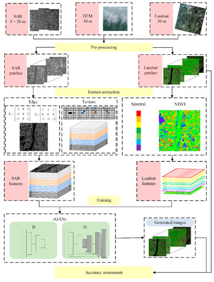
Figure 1.
Overview of the method employed in this study.
- (1)
- Preprocessing: optical remote sensing images and SAR images were preprocessed and split into small patches.
- (2)
- Feature extraction: rich spectral information of optical remote sensing images and rich structural information of SAR images were extracted as feature vectors.
- (3)
- cGANs model training: SAR-optical patches were input to train the cGANs until convergence. In this step, we input paired co-polarization SAR-optical patches, cross-polarization SAR-optical patches, and dual-polarization SAR-optical patches.
- (4)
- Accuracy assessment: neural network classification was used to classify the generated optical images and original optical images, then compare the classification results.
2.1. Paired Features for Model Training From Remote Sensing Images
In this experiment, Landsat8 multi-spectral data were used for the optical image, and Sentinel-1 data was used for the SAR image. Landsat8 was launched by the National Aeronautics and Space Administration (NASA) and the United States Geological Survey (USGS), carrying the Operational Land Imager (OLI) and Thermal Infrared Sensor (TIRS). Sentinel-1 was launched by the European Space Agency (ESA) and is composed of a constellation of two satellites, Sentinel-1A and Sentinel-1B, sharing the same orbital plane. Both satellites carry a C-band SAR sensor and provide dual-polarization SAR images in all weather conditions, day or night. We used Landsat imagery from Hengyang City, Hunan Province, China, from July to September 2018 and 2019, along with corresponding Sentinel-1 images (with a time difference of fewer than 14 days).
For optical images, Fmask (function of mask) algorithm [66,67] was used to detect the cloud regions from landsat8 data and generate the cloud mask. First, it uses Landsat top of atmosphere (TOA) reflectance and brightness temperature (BT) as inputs, and uses rules based on cloud physical properties to separate potential cloud pixels (PCPs) and clear-sky pixels. Next, a normalized temperature probability, spectral variability probability, and brightness probability are combined to produce a probability mask for clouds over land and water separately. Then, the PCPs and the cloud probability mask are used together to derive the potential cloud layer. Using the cloud mask, we were able to remove invalid cloud regions and get cloud-free regions. SAR images were subjected to the following processes: multilooking, despeckling, geocoding, radiometric calibration, and resampling. After preprocessing, we obtained large paired SAR-optical images with the same geographic coordinate system and spatial resolution (30 m). Then, we used a sliding window to split the large paired SAR-optical images into small patches with a size of 256 × 256 pixels.
To fully exploit the rich spectral information of optical remote sensing images, we used a feature vector containing the pixel spectral information from bands 1 to 7 and the normalized difference vegetation index (NDVI); therefore, the optical feature vector contained eight channels (coastal aerosol, blue, green, red, near infrared[NIR], short-wave infrared[SWIR 1, SWIR 2 ], and NDVI).
In SAR data, the radar backscatter coefficient of the ground object is strongly correlated with the grayscale feature on the image; therefore, the grayscale difference cannot effectively reflect changes in the ground object target. As such, it is necessary to introduce textural features to represent the rich structural information contained in SAR data. The gray level concurrence matrix (GLCM) was first proposed by Haralick [68] in the early 1970s. It effectively describes the image gray value in terms of the direction, stride, and space between adjacent pixels, and can be simply interpreted as an estimate of the second-order joint probability:
where and are the distance and direction, respectively, denotes the pixel point with a gray value of I, and the probability of the pixel point with a gray value of J appearing in the specified distance and direction . For simplicity, the textural features of SAR images are generally obtained using the features of correlation, contrast, homogeneity, and energy, which can effectively reflect the texture of remote sensing images [69].
In addition to textural information, the edge information also exhibits good differentiation. The edge of the image is the boundary between adjacent different homogeneous regions, which is the region with the richest amount of useful information that contains the basic features of the target structure. In this study, we used the Canny edge detection algorithm [70] to extract the edge information of the SAR image. The Canny algorithm applies a Gaussian filter for image smoothing and noise suppression, then filters out low-gradient edge pixels (caused by noise), based on a hysteresis thresholding method [71]. The specific implementation steps were as follows:
- (1)
- A Gaussian filter was used to smooth the image and filter out noise.
- (2)
- The gradient magnitude and direction of the filtered image was calculated. The direction of a pixel was divided into components in the x direction and y direction. The Canny operator was used to perform relevant operations with the original image and calculate the gradient of the pixel in the horizontal and vertical directions.
- (3)
- All values along the gradient line, except for the local maxima, were suppressed to sharpen the edge features.
- (4)
- By selecting high and low thresholds, edge pixels with weak gradient values were filtered out and edge pixels with high gradient values were retained.
For the SAR images, we computed the features using the GLCM and Canny edge detection algorithm. As shown in Figure 2, we computed four features (correlation, contrast, homogeneity, and energy) in four directions (0°, 45°, 90°, and 135°) using 7 × 7 windows. Then, each SAR pixel in co-polarization mode (VV) and cross-polarization mode (VH) was represented by a 17-dimensional feature vector, whereas those in dual-polarization mode (VV&VH) were represented by a 34-dimensional feature vector.
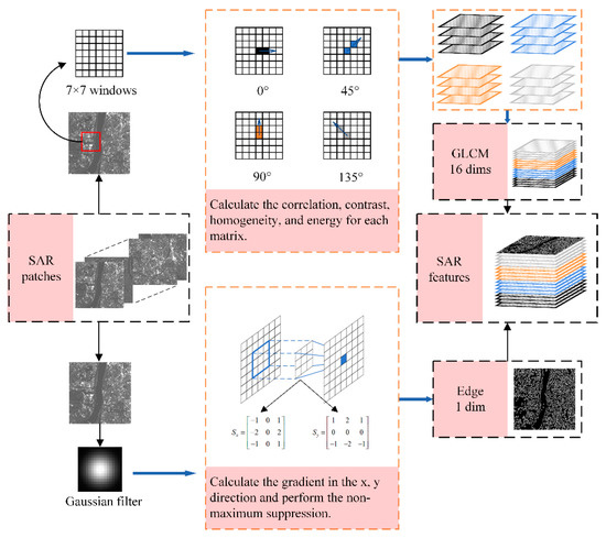
Figure 2.
Feature extraction method for synthetic-aperture radar (SAR) data.
2.2. SAR-to-Optical Translation
2.2.1. Conditional Generative Adversarial Networks (cGANs)
cGANs are an extension of the GAN concept, whereby both the generator and discriminator are conditioned using additional information (y). The loss function for conditional GANs is expressed by:
Previous studies [42] have found it favorable to combine the cGANs objective function with a loss function that measures the difference between pixels, such as the L1 distance:
Then, the whole objective function can be defined as:
where λ is a parameter that controls the weight of the L1 distance in the overall objective function.
The additional information can be any type of auxiliary information, such as class labels or data from other modalities [40]. If x and y represent two different image domains, then cGANs can achieve the corresponding image-to-image translation [48]. Many applications have exploited this characteristic for image translation [72,73]; in this study, we apply it to SAR-to-optical translation.
2.2.2. Network Architecture
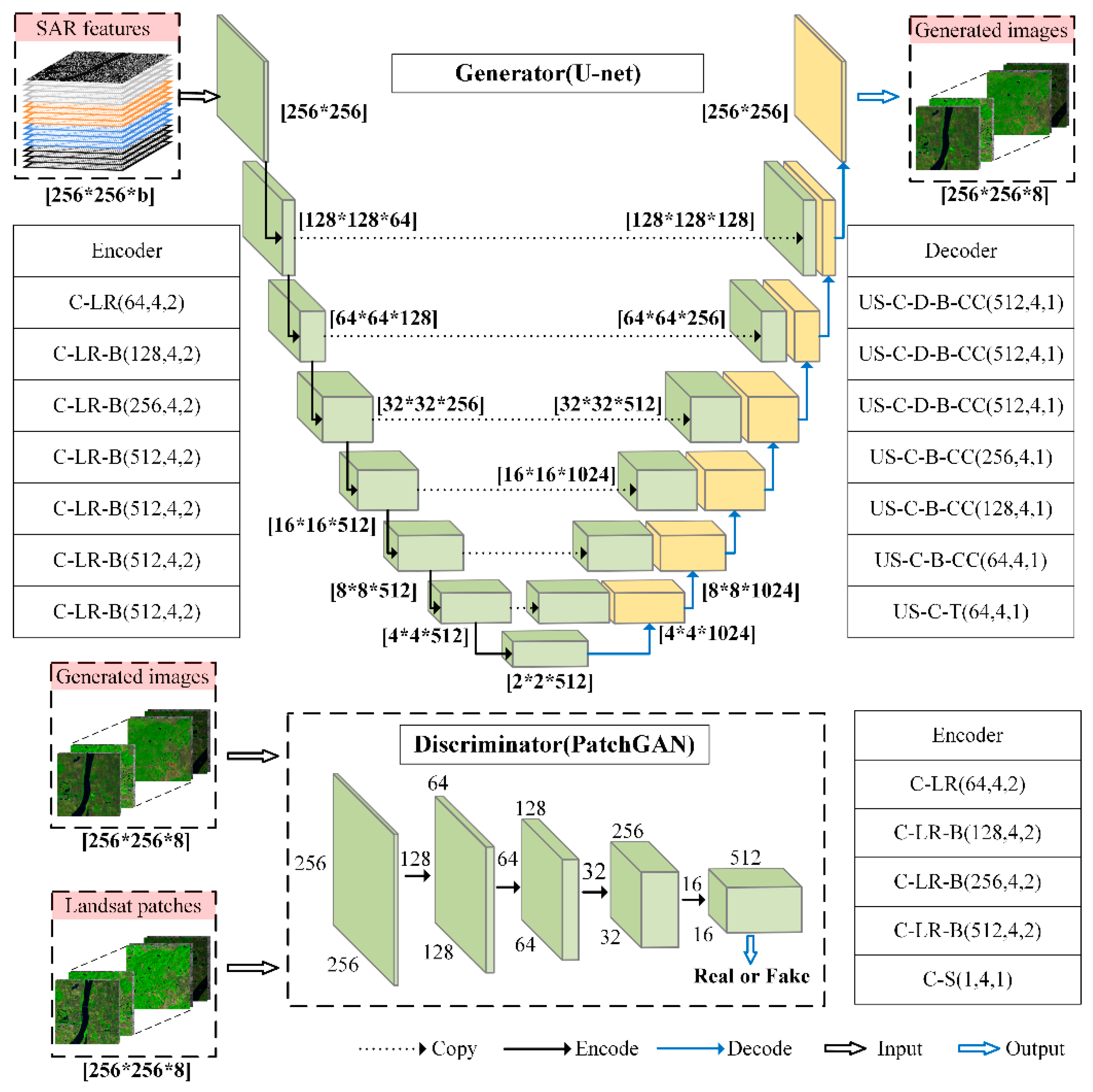
We adapted the pix2pix network architectures [48] to be compatible with multi-spectral optical images, as well as either one-channel (VV or VH) or two-channel (VV and VH) SAR images. Pix2pix, as a widely-used image-to-image translation network architecture, has proven stable and powerful for image-to-image translation [72,74]. It makes it possible to create various images without specialized knowledge of the images that we want to make [38]. In particular, the generator adopted the U-Net [75] architecture, consisting of seven convolution layers for encoding and seven deconvolution layers for decoding. In contrast, the discriminator adopted the PatchGAN architecture, consisting of five convolutional layers, followed by a sigmoid output layer for classification. The detailed information is shown in Figure 3. The inputs of the generators were SAR images, and the discriminators were either SAR images or optical images. The outputs of the generators were the generated optical images. For VV and VH polarization modes, the size of the input of the generator was set to 256 × 256 × 17, whereas for the VV&VH polarization mode, the size of the input of the generator was set to 256 × 256 × 34. The output of the generator was set to 256 × 256 × 8 and the size of the input of the discriminator was set to 256 × 256 × 16.
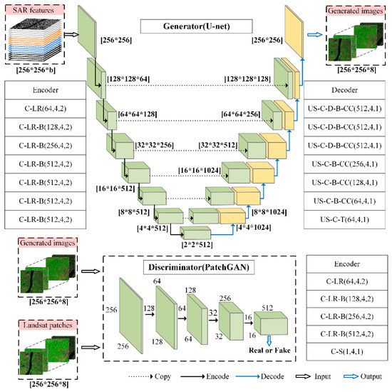
Figure 3.
Architectures of the generator networks and discriminator networks. Acronyms in the encoder and decoder units are as follows: b: number of bands, C: convolutional, LR: leaky ReLU, B: batch normalization, D: dropout, US: upsampling, CC: concatenation, T: tanh. The three numbers in round brackets shown in all encoding and decoding layers indicate the number of filters, filter size, and stride, respectively. The numbers in square brackets indicate the size of the feature maps. The discriminator learns to classify between fake (generated images, SAR patches) and real (Landsat patches, SAR patches) tuples.
2.2.3. Establishing the SAR-to-Optical Translation Relationship by Model Training
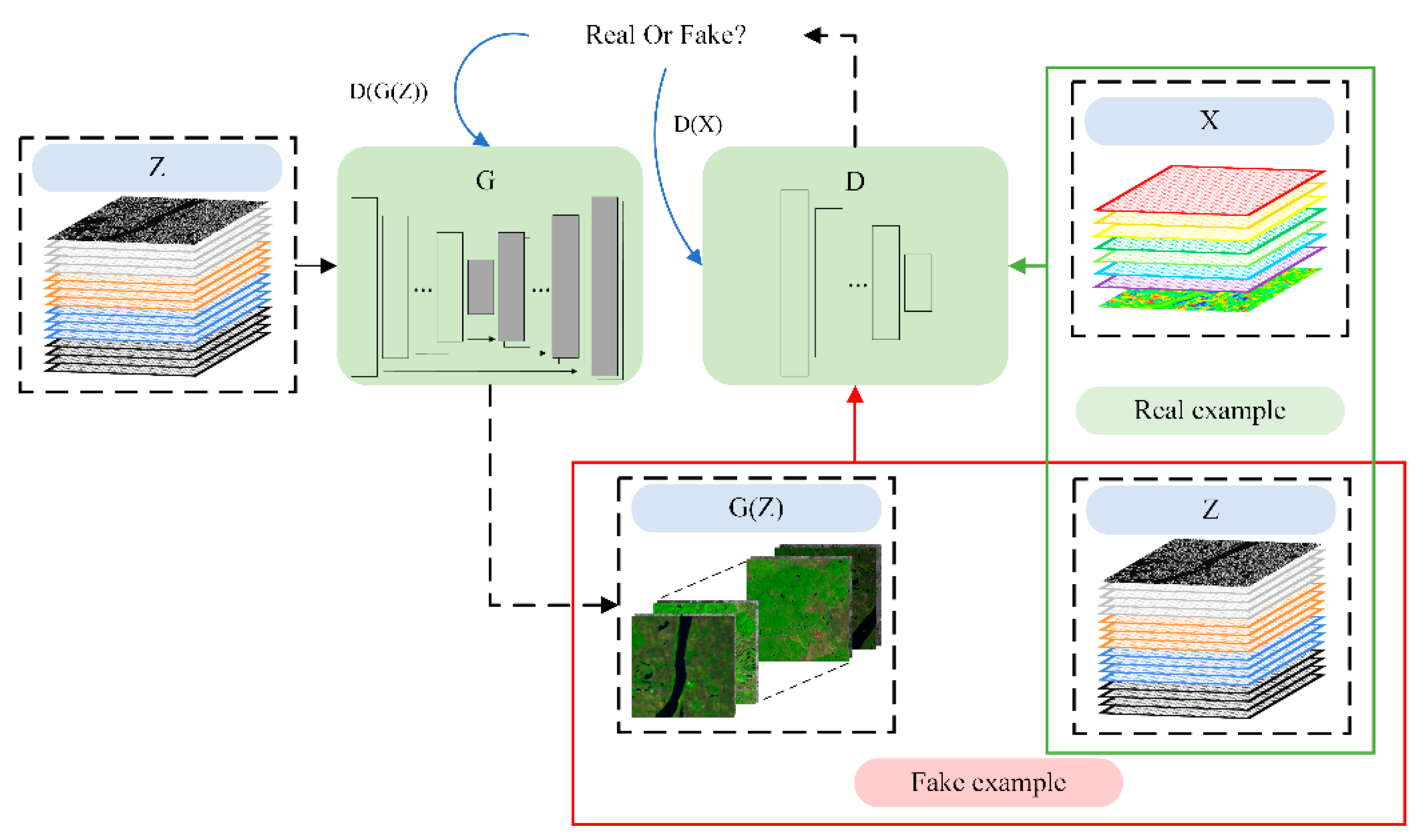
The small SAR-optical patches were input in order to train the cGANs until convergence (Figure 4). The generator uses SAR patches as the input to generate optical images. The generated images and SAR patches are then classed as fake examples, whereas the Landsat patches and SAR patches are classed as real examples for the discriminator to learn. Each time the optical image generated by the generator is judged by the discriminator, information regarding its judgment is fed back to the generator. When the discriminator is unable to determine whether the input data patches are real or fake, it indicates that the images generated by the generator are good enough, and the training is ended. The training parameters at this point correspond to the SAR- to-optical relationship

Figure 4.
Training process of the proposed method. G: generator; D: discriminator; Z: SAR features; X: Landsat features; G (Z): image generated by the generator; D(G(Z)): feedback from the fake example; D(X): feedback from the real example. The red box denotes the training setup for fake examples (generated images, SAR patches) as the input, and the green box denotes the training setup for real examples (Landsat patches, SAR patches) as the input.
In this step, we input the paired co-polarization SAR(VV)-optical images, cross-polarization SAR(VH)-optical images, and dual-polarization SAR(VV&VH)-optical images. For each polarization mode, we extracted 2300 pairs of patches, of which 1700 pairs were classed as training data, among which 600 pairs were the most common testing data, which trained 200 epochs at a batch size of 16. The networks were trained with stochastic gradient descent and the ADAM optimizer [76], where the learning rate was set to 0.0002 and β was set to 0.5. All code development was conducted with TensorFlow deep learning frameworks on the Ubuntu operating system, and training was conducted on a single Graphic Processing Unit(GPU),namely, NVIDIA Tesla P100.
2.2.4. Optical Image Generation
Once the SAR-to-optical translation relationship was determined, i.e., by obtaining the training parameters at the point when the model converges, we used this relationship to generate the optical image. In reality, we already had the original optical image at time T1 (the real image) but pretended otherwise, for convenience of verification. Then, we used the SAR image at time T1 as the input and generated the optical image at time T1, using the established SAR-to-optical transformation relationship.
2.3. Evaluation of Reconstruction Image Data Quality
Neural network classification was used to classify the generated optical images and the original optical images, then compare the classification results. To quantitatively evaluate the accuracy, surface objects were visually compared using the following indicators: the peak signal-to-noise ratio (PSNR), structural similarity index measure (SSIM), correlation coefficient (r), and root mean squared error (RMSE). PSNR indicates image pixel statistical information, with a higher PSNR generally indicating higher image quality. SSIM represents structural information by calculating the structural similarity between generated images and real optical images. Its value ranges from zero to one and will reach one when the two images are identical. PSNR and SSIM are commonly used in the field of image quality evaluation. The correlation coefficient, r, is a statistical index that determines the degree of linear correlation between variables; a larger r indicates a greater relevance of the value of each pixel in the generated images real images. RMSE measures the deviation of generated values from the true value and detects the consistency between the two values; the smaller the RMSE, the denser the data and the higher the quality of the generated image.
3. Results
3.1. Influence of Edge Information on SAR-to-Optical Translation
In this experiment, we compare the influence of the addition of edge information on the SAR-to-optical translation process without comparing different polarization modes. We perform control experiments using only the textural information as the input; the textural information is provided by the GLCM and the edge information is provided by the Canny edge detection algorithm.
3.1.1. Qualitative Evaluation of Generated Images
The results generated from several different inputs are compared with the original images in Figure 5. From the perspective of visual effects, after the addition of the edge information, the boundaries of the water body are clearer and more continuous. Specifically, in VV mode (as shown in the vertical comparison of columns 2 of Figure 5), the addition of edge information results in blurrier ground objects with less textural information in the generated image; in VH mode (as shown in the vertical comparison of columns 3 of Figure 5), the addition of edge information results in a clearer boundary between the water body and vegetation in the generated image, as well as more detailed textural information; in VV&VH mode (as shown in the vertical comparison of columns 4 of Figure 5), the addition of edge information also results in a clearer boundary between the water body and vegetation in the generated image, as well as a more uniform water body that does not erroneously contain vegetation.
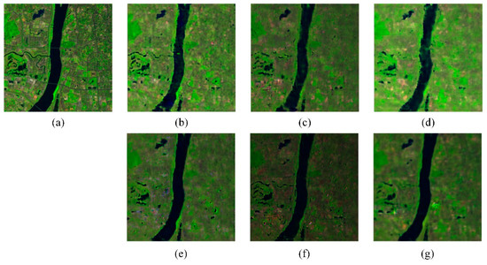
Figure 5.
Comparison of generated results. (a): real image; (b): VV-GLCM; (c): VH-GLCM; (d): VV&VH-GLCM; (e): VV- GLCM&Canny; (f): VH- GLCM&Canny; (g): VV&VH- GLCM&Canny. Acronyms indicate images generated using: VV: co-polarization as the input; VH: cross-polarization as the input; VV&VH: dual-polarization as the input; gray level concurrence matrix (GLCM): only textural information as the input; GLCM&Canny: both textural information and edge information as the input.
3.1.2. Quantitative Evaluation of Generated Images
Table 1 shows the image quality assessment (IQA) results for the different combinations of inputs. The best values for each quality index are shown in bold. The IQA consists of PSNR and SSIM. After edge information is added, images generated using the VV mode input exhibit lower quality according to both indexes, indicating that the addition of edge information in this case results in a more confusing cGANs with weaker learning ability. Conversely, images generated using the VH mode input exhibit higher quality; however, this improvement is only observed in bands 1, 2, and 7 for PSNR, indicating that the addition of edge information in this case may provide the cGANs with more effective information. Furthermore, images generated using the VV&VH mode input improve in all bands for both indexes, indicating that the addition of edge information in this case provides the cGANs with more effective information and results in better image quality. It is worth noting that the SSIM is improved for images generated using the VV and VV&VH polarization modes, which indicates that the generated images are more similar to the real image in terms of brightness, contrast, and structure.

Table 1.
Image quality assessment (IQA) results of different inputs. The best values for each quality index are shown in bold.
3.2. Comparison of Different Polarization Modes
In this experiment, we compare the optimal polarization of the three polarization modes in two cases: (1) using both textural information and edge information as the input and (2) using only textural information as the input. To quantitatively assess the accuracy of the images generated by the different polarization modes, we employ the r and RMSE values between the predicted reflectance and real reflectance. To display the result clearly, we employ a scatter diagram to show the density distribution of data using MATLAB. The scatter diagram shows the reflectance relationship between the generated values and the actual values of the Landsat image, where the line in the scatter diagram is the 1:1 line. Points that are close to the line indicate that the algorithm can capture the reflectance change in surface objects and achieve high accuracy in predicting the reflectance of pixels. The yellow color indicates high centralization of points.
3.2.1. Optimal Polarization Mode Using Textural Information and Edge Information
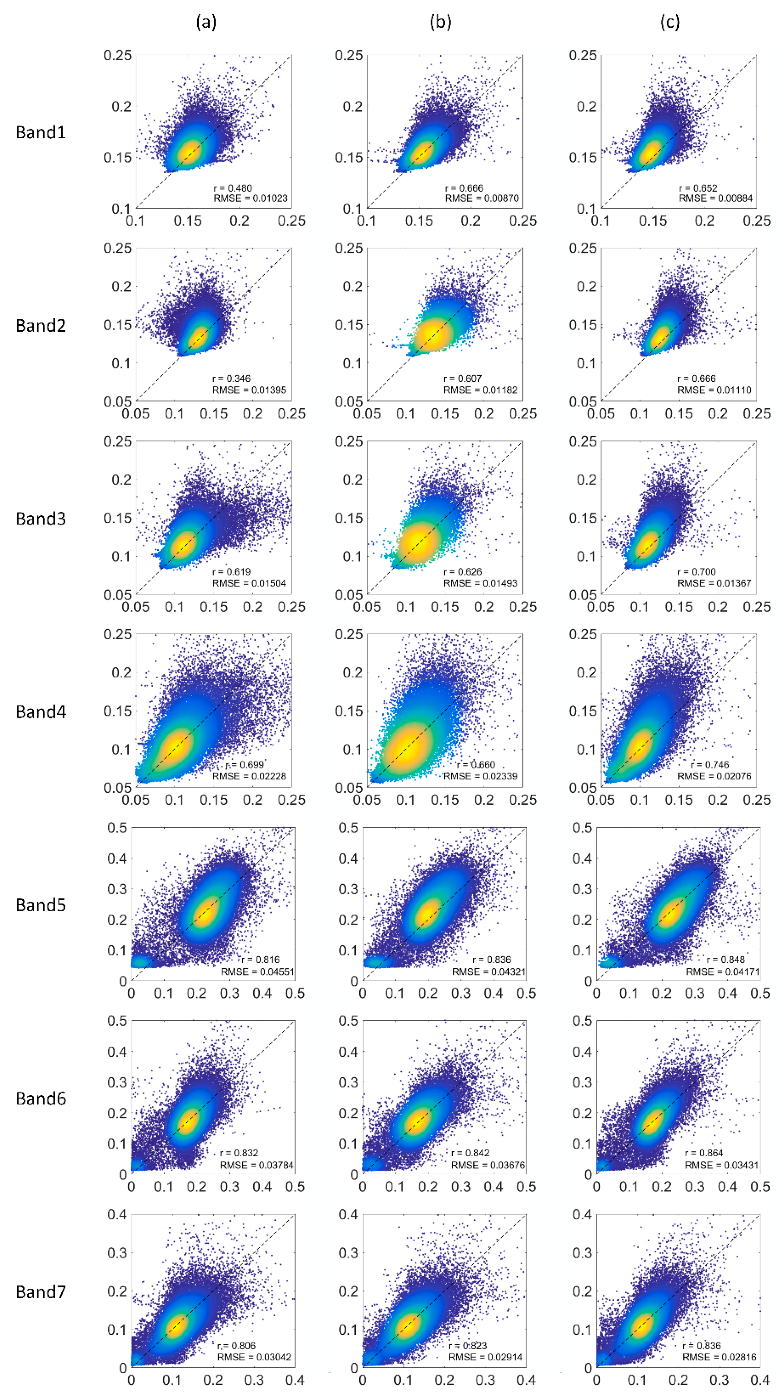
According to the statistical data, images generated using the VV&VH polarization mode achieve the best r and RMSE values, followed by images generated using VH polarization, with those generated using VV polarization achieving the worst r and RMSE values. Regardless of the polarization mode used as the input, the r value is higher for bands 5–7 than bands 1–4, with band 6 exhibiting the highest r value (VV: r = 0.832, VH: r = 0.842, VV&VH: r = 0.864) and band 2 in images generated using VV and VH polarization exhibiting the lowest r value (VV: r = 0.346, VH: r = 0.607). The r value for images generated using VV&VH polarization is lowest in band 1 (r = 0.652). The relatively low r value for bands 1 and 2 under VV polarization (0.48 and 0.346, respectively) indicates that a large number of pixels have low accuracy; therefore, it is not recommended to use the VV polarization mode as the input when generating Landsat8 first band and second band images.
According to the scatter diagram (Figure 6), the reflectivity distribution for images generated using VV&VH polarization as the input is relatively concentrated, with the majority of data falling in the yellow area and light blue area, and relatively little data in the low-density dark blue area. In comparison, although the high-density yellow area is larger for images generated using VH polarization as the input, more low-density points appear in the dark blue area. Finally, the reflectivity values of images generated using VV polarization as the input exhibit a relatively discrete distribution, with a large number of low-density dark blue points falling far from the 1:1 fitting line.
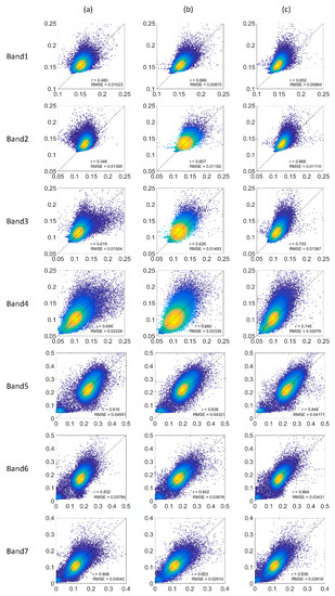
Figure 6.
Scatter plots of the real reflectance and generated reflectance produced by co-polarization (VV), cross-polarization (VH), and dual-polarization (VV&VH) inputs when both textural information and edge information are input. (a): co-polarization (VV); (b): cross-polarization (VH), (c): dual-polarization (VV&VH). The horizontal axis represents the generated values, the vertical axis represents the actual values, r represents the correlation between the generated values and actual values, and RMSE represents the root mean square error.
3.2.2. Optimal Polarization Mode Using only Textural Information
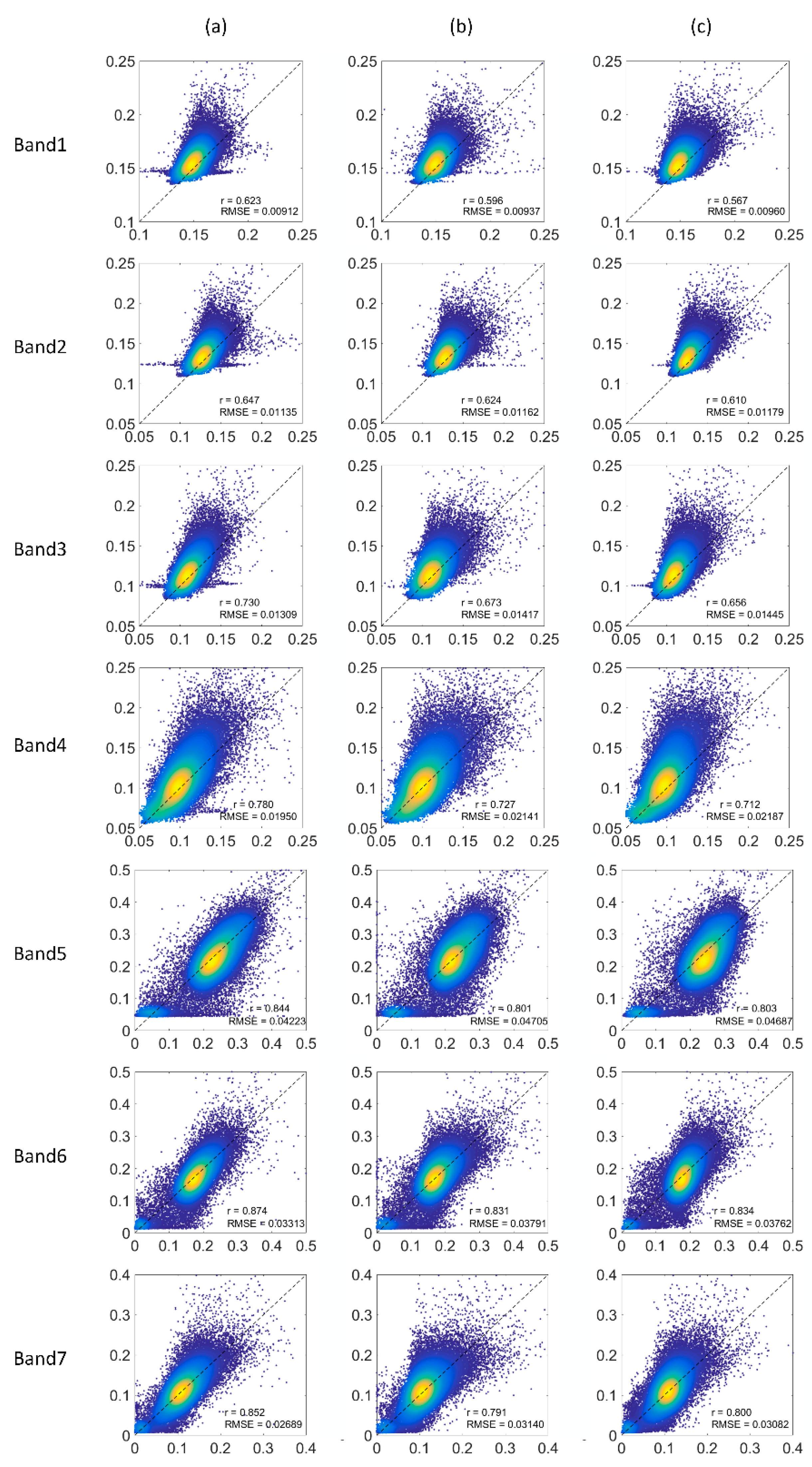
According to the statistical data, the images generated using the VV polarization mode as the input exhibit the best r and RMSE values, followed by those generated using VV&VH polarization, with images generated using VH polarization exhibiting the worst r and RMSE values. Again, regardless of the polarization mode, bands 5–7 exhibit higher r values than bands 1–4, with the highest r value in band 6 (VV: r = 0.874, VH: r = 0.831, VV&VH: r = 0.834) and the lowest r value in band 1 (VV: r = 0.623, VH: r = 0.596, VV&VH: r = 0.567).
According to the scatter diagram (Figure 7), the reflectivity distribution for images generated using the VV polarization mode is relatively small, but some points are scattered parallel to the X-axis in bands 1–4. Taking band 1 as an example, some points appear near the y = 0.15 line, which indicates that points with a reflectance of 0.15 in the real image are generated by mistake with values ranging from 0.10 to 0.18. This situation is alleviated when the image is generated using the VH polarization mode as the input, and almost disappears when the image is generated using the VV&VH polarization mode as the input.

Figure 7.
Scatter plots of the real reflectance and generated reflectance produced by co-polarization (VV), cross-polarization (VH), and dual-polarization (VV&VH) inputs when only textural information are input. (a): co-polarization (VV); (b): cross-polarization (VH), (c): dual-polarization (VV&VH). The horizontal axis represents the generated values, the vertical axis represents the actual values, r represents the correlation between generated values and actual values, and RMSE represents the root mean square error.
3.3. Accuracy Evaluation of Optimal Input Features for Different Surface Objects
3.3.1. Classification and Area Ratio Comparison
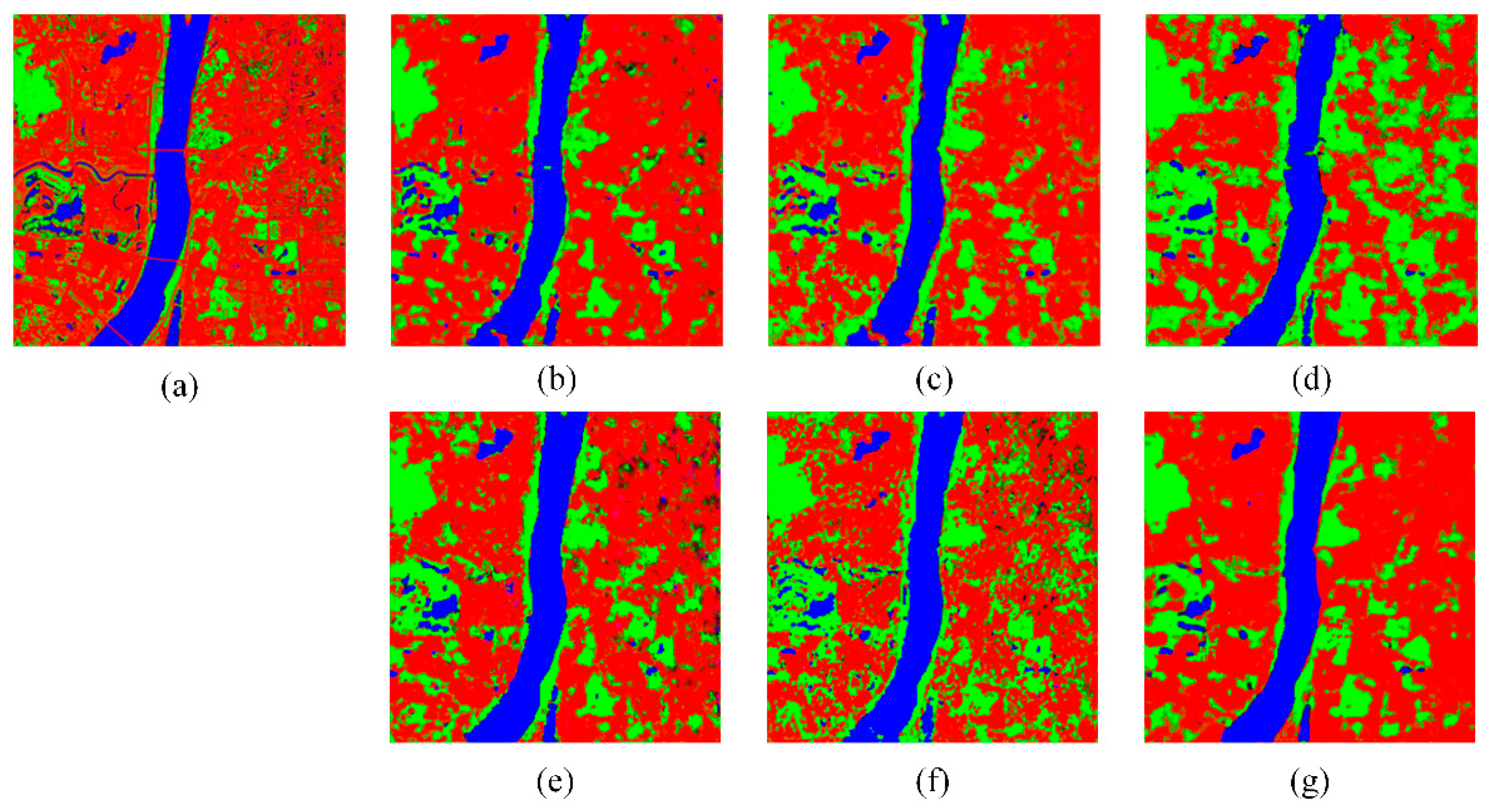
To assess the accuracy of surface object information in the generated images, we classify the generated images into three categories: water bodies, building land, and vegetation, and determine the areal proportion of each surface object (Table 2). The proportions of the three types of surface object in the real images are regarded as the baseline for the other sets. The best values for each quality index are shown in bold. Figure 8 shows the intuitive results of the classification. When only the GLCM is used as the input, the classification results of VV polarization are closest to those of the real images. When both the GLCM and edge information are used as the input, the classification results of VV&VH polarization are closest to those of the real images.

Table 2.
Areal proportion of different classification results. The best values for each quality index are shown in bold.

Figure 8.
Comparison of surface object classification results. (a): real image; (b): VV-GLCM; (c): VH-GLCM; (d): VV&VH-GLCM; (e): VV- GLCM&Canny; (f): VH- GLCM&Canny; (g): VV&VH- GLCM&Canny. Acronyms indicate images generated with: VV: co-polarization as the input; VH: cross-polarization as the input; VV&VH: dual-polarization as the input; GLCM: only textural information as the input; GLCM&Canny: both textural information and edge information as the input. Blue represents water bodies, red represents building land, and green represents vegetation.
In VV polarization mode, the addition of edge information results in finer classification of surface object patches, which means that the generated images contain more detailed information. Water bodies surrounded by vegetation and building land are also effectively distinguished; thus, the water area is closer to that in the real image. However, many pixels that should be classified as building land are misclassified as vegetation, resulting in a smaller proportion of building land and a higher proportion of vegetation compared to the real image. The VH polarization results are similar to those of VV polarization, except that the addition of edge information results in better separation of water bodies and more detailed water area information in the generated image. In VV&VH polarization mode, the addition of edge information again makes the water boundaries more continuous and clear, reduces the misclassification of building land and vegetation, and generates areal proportions that are more similar to those in the real images for all three surface objects.
3.3.2. Correlation Comparison
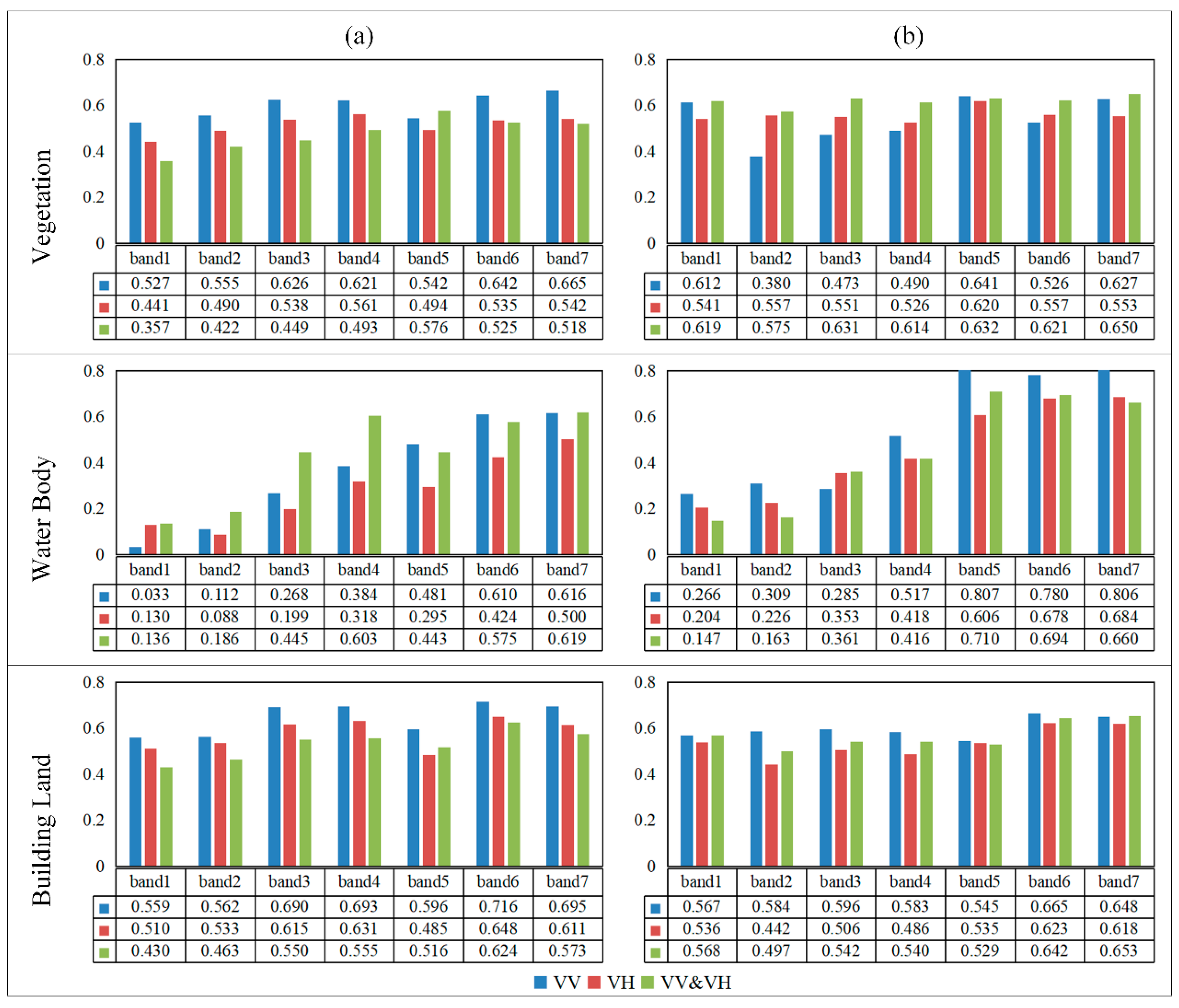
The scattering mechanism of SAR data is divided into surface scattering, body scattering, double echo, etc., which gives the SAR images different backscattering intensity for different surface objects. Therefore, we determine the optimal input for different types of surface objects by calculating the r value between the generated image and the original image for different surface objects (Figure 9). For vegetation, the VV&VH polarization mode with edge information is the optimal input. Although the overall correlation for the VV polarization mode without edge information is relatively high, the correlation of each band is quite different. With the addition of edge information, the correlation is improved for vegetation areas generated with VH and VV&VH polarization modes as the input. For water bodies, the VV polarization mode with edge information is the optimal input, which may be because backscattering of the water body is typically surface reflection, which requires a polarization mode with a stronger echo, such as the VV polarization mode. The addition of edge information significantly improves the correlation for water body areas generated using each polarization mode. For building land, the VV polarization mode without edge information is the optimal input. The addition of edge information improves the correlation for building land generated using VV&VH polarization. Therefore, different input features should be selected for different types of surface object to ensure optimal image accuracy.
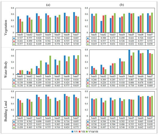
Figure 9.
Correlation bar chart of each band under different polarization modes: (a) without edge information, (b) with edge information. The horizontal axis represents the different bands and the vertical axis represents the correlation coefficient.
4. Discussion
4.1. Effects of Different Reconstruction Methods on Different Optical Bands
There are many methods available for reconstructing optical remote sensing images [77,78,79,80,81,82]. The cGANs method adopted in this study has great potential for the reconstruction of NIR and SWIR bands (for Landsat8 images, band 5 is the NIR band, and bands 6 and 7 are the SWIR bands). For example, the spatial and temporal adaptive reflectance fusion model (STARFM) was used to obtain r values for NIR and SWIR bands of 0.693, 0.598, and 0.638, respectively [82], whereas the r values obtained in our study for inputs including edge information, textural information, and the VV&VH polarization mode were 0.848, 0.864, and 0.836, respectively. Moreover, sparse representation was used to reconstruct an optical image with a PSNR value for band 5 of 22.35 [8], whereas our study obtained a PSNR value of 27.33. Finally, the improved spatial-temporal fusion method was used to predict a reflectance r value for band 5 of 0.8403 [83], whereas the r value obtained in our study was 0.848. NIR and SWIR bands are typically used for urban monitoring, detection, and identification of roads, exposed soil, and water. Therefore, cGANs-based SAR-to-optical image translation methods may be the most suitable for image generation in these cases.
4.2. Superior Reconstruction with an Adequate Textural Extraction Scale
In this study, we used the GLCM to extract textural features, and the size of the running window was set to 7 × 7. However, different ground objects do not have the same texture size, periodic mode, or direction; therefore, the window size of 7 × 7 may not be suitable for all ground objects. This highlights a very interesting problem, that is, the problem of textural scale or the size of the window involved in the texture extraction process. Many previous studies have demonstrated that the textural scale has a significant influence on image reconstruction [84,85]. A larger textural scale can lead to blurred boundaries and interiors of the textural information and even mosaic phenomena, which conceals relatively small changes in the image. Conversely, a smaller textural scale will result in a more broken and spotted image, despite the more detailed textural information, which is not conducive to subsequent surface object extraction. Therefore, the spectral properties and spatial properties of the geological phenomena or processes being studied should be considered when selecting the textural scale. However, this topic is beyond the scope of this study.
5. Conclusions
In this study, we translated SAR images into optical images using cGANs, then investigated the effect of adding edge information and using three different polarization modes in the model input on the translation process. The major findings are as follows.
The addition of edge information improves the structural similarity between the generated image and the real image, makes the boundaries between surface objects clearer in the generated image, and provides the cGANs with more effective information, resulting in better image quality when VH and VV&VH polarization modes are used as the input. The optimal polarization mode with edge information added in the input is VV&VH, whereas the optimal polarization mode without edge information is VV. Moreover, different surface object types have different optimal input features. For example, VV&VH polarization with edge information is the optimal input for vegetation, VV polarization with edge information is the optimal input for water bodies, and VV polarization without edge information is the optimal input for building land. Overall, the accuracy of NIR and SWIR bands in the generated image is higher than that of visible bands (for Landsat8 images, bands 5–7 are more accurate than bands 2–4).
These findings provide an important reference for the selection of cGANs input features and have important applications for cloud removal, vegetation index reconstruction, etc. Although we only translated Sentinel-1 images into Landsat8 images, the translation of other optical images and SAR images is also theoretically feasible. Our results indicate that SAR-to-optical image translation can generate high-quality optical images that can be used in the construction of high temporal and spectral resolution time-series data. Future research should consider using images from multiple satellites and introducing time-series data to further improve the translation results.
Author Contributions
Conceptualization: Q.Z., X.L., and M.L.; methodology: Q.Z.; software: Q.Z.; validation: Q.Z. and X.Z.; formal analysis: Q.Z. and X.Z.; investigation: Q.Z.; resources: Q.Z. and X.R.; data curation: Q.Z.; writing—original draft preparation: Q.Z.; writing—review and editing: Q.Z., X.Z., M.L., and L.Z.; visualization: Q.Z.; supervision: X.L. and M.L.; project administration: X.L.; funding acquisition: X.L. All authors have read and agreed to the published version of the manuscript.
Funding
This research was funded by the National Natural Science Foundation of China under Grant 41871223.
Institutional Review Board Statement
Not applicable.
Informed Consent Statement
Not applicable.
Data Availability Statement
Data sharing not applicable.
Conflicts of Interest
The authors declare no conflict of interest.
References
- Melgani, F.; Bruzzone, L. Classification of hyperspectral remote sensing images with support vector machines. IEEE Trans. Geosci. Remote Sens. 2004, 42, 1778–1790. [Google Scholar] [CrossRef]
- Zhang, J.; Zhong, P.; Chen, Y.; Li, S. L-1/2-Regularized Deconvolution Network for the Representation and Restoration of Optical Remote Sensing Images. IEEE Trans. Geosci. Remote Sens. 2014, 52, 2617–2627. [Google Scholar] [CrossRef]
- Hasituya; Chen, Z.; Li, F.; Hongmei. Mapping Plastic-Mulched Farmland with C-Band Full Polarization SAR Remote Sensing Data. Remote Sens. 2017, 9, 1264. [Google Scholar] [CrossRef]
- Meng, Y.; Liu, X.; Ding, C.; Xu, B.; Zhou, G.; Zhu, L. Analysis of ecological resilience to evaluate the inherent maintenance capacity of a forest ecosystem using a dense Landsat time series. Ecol. Inf. 2020, 57. [Google Scholar] [CrossRef]
- Inglada, J.; Vincent, A.; Arias, M.; Marais-Sicre, C. Improved Early Crop Type Identification By Joint Use of High Temporal Resolution SAR And Optical Image Time Series. Remote Sens. 2016, 8, 362. [Google Scholar] [CrossRef]
- He, W.; Yokoya, N. Multi-Temporal Sentinel-1 and-2 Data Fusion for Optical Image Simulation. ISPRS Int. J. Geo-Inf. 2018, 7, 389. [Google Scholar] [CrossRef]
- Li, Z.; Shen, H.; Cheng, Q.; Liu, Y.; You, S.; He, Z. Deep learning based cloud detection for medium and high resolution remote sensing images of different sensors. ISPRS J. Photogramm. Remote Sens. 2019, 150, 197–212. [Google Scholar] [CrossRef]
- Huang, B.; Li, Y.; Han, X.; Cui, Y.; Li, W.; Li, R. Cloud Removal From Optical Satellite Imagery With SAR Imagery Using Sparse Representation. IEEE Geosci. Remote Sens. Lett. 2015, 12, 1046–1050. [Google Scholar] [CrossRef]
- Li, Y.; Li, W.; Shen, C. Removal of Optically Thick Clouds From High-Resolution Satellite Imagery Using Dictionary Group Learning and Interdictionary Nonlocal Joint Sparse Coding. IEEE J. Sel. Top. Appl. Earth Obs. Remote Sens. 2017, 10, 1870–1882. [Google Scholar] [CrossRef]
- Shang, R.; Wang, J.; Jiao, L.; Stolkin, R.; Hou, B.; Li, Y. SAR Targets Classification Based on Deep Memory Convolution Neural Networks and Transfer Parameters. IEEE J. Sel. Top. Appl. Earth Obs. Remote Sens. 2018, 11, 2834–2846. [Google Scholar] [CrossRef]
- Larranaga, A.; Alvarez-Mozos, J. On the Added Value of Quad-Pol Data in a Multi-Temporal Crop Classification Framework Based on RADARSAT-2 Imagery. Remote Sens. 2016, 8, 335. [Google Scholar] [CrossRef]
- Hasituya; Chen, Z.; Li, F.; Hu, Y. Mapping plastic-mulched farmland by coupling optical and synthetic aperture radar remote sensing. Int. J. Remote Sens. 2020, 41, 7757–7778. [Google Scholar] [CrossRef]
- Haupt, S.; Engelbrecht, J.; Kemp, J. Predicting MODIS EVI from SAR Parameters Using Random Forests Algorithms. In Proceedings of the IEEE International Geoscience & Remote Sensing Symposium, Fort Worth, TX, USA, 23–28 July 2017; pp. 4382–4385. [Google Scholar]
- Hertzmann, A.; Jacobs, C.E.; Oliver, N.; Curless, B.; Salesin, D.H.; Acm, A.C.M. Image analogies. In Proceedings of the SIGGRAPH01: The 28th International Conference on Computer Graphics and Interactive Techniques, Los Angeles, CA, USA, 12–17 August 2001; pp. 327–340. [Google Scholar]
- Alotaibi, A. Deep Generative Adversarial Networks for Image-to-Image Translation: A Review. Symmetry 2020, 12, 1705. [Google Scholar] [CrossRef]
- Li, Y.; Fu, R.; Meng, X.; Jin, W.; Shao, F. A SAR-to-Optical Image Translation Method Based on Conditional Generation Adversarial Network (cGAN). IEEE Access 2020, 8, 60338–60343. [Google Scholar] [CrossRef]
- Zhang, W.; Xu, M. Translate SAR Data into Optical Image Using IHS and Wavelet Transform Integrated Fusion. J. Indian Soc. Remote Sens. 2019, 47, 125–137. [Google Scholar] [CrossRef]
- Eckardt, R.; Berger, C.; Thiel, C.; Schmullius, C. Removal of Optically Thick Clouds from Multi-Spectral Satellite Images Using Multi-Frequency SAR Data. Remote Sens. 2013, 5, 2973–3006. [Google Scholar] [CrossRef]
- Liu, L.; Lei, B. Can SAR Images and Optical Images Transfer with Each Other? In Proceedings of the 38th IEEE International Geoscience and Remote Sensing Symposium (IGARSS), Valencia, Spain, 22–27 July 2018; pp. 7019–7022. [Google Scholar]
- Reyes, M.F.; Auer, S.; Merkle, N.; Henry, C.; Schmitt, M. SAR-to-Optical Image Translation Based on Conditional Generative Adversarial Networks-Optimization, Opportunities and Limits. Remote Sens. 2019, 11, 2067. [Google Scholar] [CrossRef]
- Merkle, N.; Mueller, R.; Reinartz, P. Registration og Optical and SAR Satellite Images Based on Geometric Feature Templates. In Proceedings of the International Conference on Sensors and Models in Remote Sensing and Photogrammetry, Kish Island, Iran, 23–25 November 2015; pp. 447–452. [Google Scholar]
- Chen, M.; Habib, A.; He, H.; Zhu, Q.; Zhang, W. Robust Feature Matching Method for SAR and Optical Images by Using Gaussian-Gamma-Shaped Bi-Windows-Based Descriptor and Geometric Constraint. Remote Sens. 2017, 9, 882. [Google Scholar] [CrossRef]
- Polcari, M.; Tolomei, C.; Bignami, C.; Stramondo, S. SAR and Optical Data Comparison for Detecting Co-Seismic Slip and Induced Phenomena during the 2018 M-w 7.5 Sulawesi Earthquake. Sensors 2019, 19, 3976. [Google Scholar] [CrossRef]
- Schmitt, M.; Hughes, L.H.; Körner, M.; Zhu, X.X. Colorizing Sentinel-1 SAR Images Using a Variational Autoencoder Conditioned on Sentinel-2 Imagery. Int. Arch. Photogramm. Remote Sens. Spatial Inf. Sci. 2018, XLII-2, 1045–1051. [Google Scholar] [CrossRef]
- Schmitt, M.; Hughes, L.H.; Zhu, X.X. The Sen1-2 Dataset for Deep Learning in Sar-Optical Data Fusion. ISPRS Ann. Photogramm. Remote Sens. Spatial Inf. Sci 2018, IV-1, 141–146. [Google Scholar] [CrossRef]
- Forkuor, G.; Conrad, C.; Thiel, M.; Ullmann, T.; Zoungrana, E. Integration of Optical and Synthetic Aperture Radar Imagery for Improving Crop Mapping in Northwestern Benin, West Africa. Remote Sens. 2014, 6, 6472–6499. [Google Scholar] [CrossRef]
- Xu, R.; Zhang, H.; Lin, H. Urban Impervious Surfaces Estimation From Optical and SAR Imagery: A Comprehensive Comparison. IEEE J. Sel. Top. Appl. Earth Obs. Remote Sens. 2017, 10, 4010–4021. [Google Scholar] [CrossRef]
- Zhang, H.; Wan, L.; Wang, T.; Lin, Y.; Lin, H.; Zheng, Z. Impervious Surface Estimation From Optical and Polarimetric SAR Data Using Small-Patched Deep Convolutional Networks: A Comparative Study. IEEE J. Sel. Top. Appl. Earth Obs. Remote Sens. 2019, 12, 2374–2387. [Google Scholar] [CrossRef]
- Auer, S.; Hornig, I.; Schmitt, M.; Reinartz, P. Simulation-Based Interpretation and Alignment of High-Resolution Optical and SAR Images. IEEE J. Sel. Top. Appl. Earth Obs. Remote Sens. 2017, 10, 4779–4793. [Google Scholar] [CrossRef]
- He, C.; Fang, P.; Xiong, D.; Wang, W.; Liao, M. A Point Pattern Chamfer Registration of Optical and SAR Images Based on Mesh Grids. Remote Sens. 2018, 10, 1837. [Google Scholar] [CrossRef]
- Merkle, N.; Luo, W.; Auer, S.; Mueller, R.; Urtasun, R. Exploiting Deep Matching and SAR Data for the Geo-Localization Accuracy Improvement of Optical Satellite Images. Remote Sens. 2017, 9, 586. [Google Scholar] [CrossRef]
- Liu, S.; Qi, Z.; Li, X.; Yeh, A.G.-O. Integration of Convolutional Neural Networks and Object-Based Post-Classification Refinement for Land Use and Land Cover Mapping with Optical and SAR Data. Remote Sens. 2019, 11, 690. [Google Scholar] [CrossRef]
- Molijn, R.A.; Iannini, L.; Rocha, J.V.; Hanssen, R.F. Sugarcane Productivity Mapping through C-Band and L-Band SAR and Optical Satellite Imagery. Remote Sens. 2019, 11, 1109. [Google Scholar] [CrossRef]
- Zhang, Y.; Zhang, H.; Lin, H. Improving the impervious surface estimation with combined use of optical and SAR remote sensing images. Remote Sens. Environ. 2014, 141, 155–167. [Google Scholar] [CrossRef]
- Zhang, L.; Zhang, L.; Du, B. Deep Learning for Remote Sensing Data: A Technical Tutorial on the State of the Art. IEEE Geosci. Remote Sens. Mag. 2016, 4, 22–40. [Google Scholar] [CrossRef]
- Long, J.; Shelhamer, E.; Darrell, T. Fully Convolutional Networks for Semantic Segmentation. In Proceedings of the IEEE Conference on Computer Vision and Pattern Recognition (CVPR), Boston, MA, USA, 7–12 June 2015; pp. 3431–3440. [Google Scholar]
- Goodfellow, I.J.; Pouget-Abadie, J.; Mirza, M.; Xu, B.; Warde-Farley, D.; Ozair, S.; Courville, A.; Bengio, Y. Generative Adversarial Nets. In Proceedings of the 28th Conference on Neural Information Processing Systems (NIPS) Montreal, Montreal, QC, Canada, 8–13 December 2014. [Google Scholar]
- Kim, S.; Suh, D.Y. Recursive Conditional Generative Adversarial Networks for Video Transformation. IEEE Access 2019, 7, 37807–37821. [Google Scholar] [CrossRef]
- Niu, X.; Gong, M.; Zhan, T.; Yang, Y. A Conditional Adversarial Network for Change Detection in Heterogeneous Images. IEEE Geosci. Remote Sens. Lett. 2019, 16, 45–49. [Google Scholar] [CrossRef]
- Mirza, M.; Osindero, S. Conditional Generative Adversarial Nets. arXiv 2014, arXiv:1411.1784. [Google Scholar]
- Grohnfeldt, C.; Schmitt, M.; Zhu, X.X. A conditional generative adversarial network to fuse SAR and multispectral optical data for cloud removal from Sentinel-2 images. In Proceedings of the 38th IEEE International Geoscience and Remote Sensing Symposium (IGARSS), Valencia, Spain, 22–27 July 2018. [Google Scholar]
- Pathak, D.; Krahenbuhl, P.; Donahue, J.; Darrell, T.; Efros, A.A. Context Encoders: Feature Learning by Inpainting. In Proceedings of the 2016 IEEE Conference on Computer Vision and Pattern Recognition (CVPR), Seattle, WA, USA, 27–30 June 2016; pp. 2536–2544. [Google Scholar]
- Xu, L.; Zeng, X.; Li, W.; Huang, Z. Multi-granularity generative adversarial nets with reconstructive sampling for image inpainting. Neurocomputing 2020, 402, 220–234. [Google Scholar] [CrossRef]
- Yuan, L.; Ruan, C.; Hu, H.; Chen, D. Image Inpainting Based on Patch-GANs. IEEE Access 2019, 7, 46411–46421. [Google Scholar] [CrossRef]
- Zhang, Z.; Song, Y.; Qi, H. Age Progression/Regression by Conditional Adversarial Autoencoder. In Proceedings of the 30th IEEE/CVF Conference on Computer Vision and Pattern Recognition (CVPR), Honolulu, HI, USA, 21–26 July 2017; pp. 4352–4360. [Google Scholar]
- Sage, A.; Agustsson, E.; Timofte, R.; Van Gool, L. Logo Synthesis and Manipulation with Clustered Generative Adversarial Networks. In Proceedings of the 31st IEEE/CVF Conference on Computer Vision and Pattern Recognition (CVPR), Salt Lake City, UT, USA, 18–23 June 2018; pp. 5879–5888. [Google Scholar]
- Wang, T.-C.; Liu, M.-Y.; Zhu, J.-Y.; Tao, A.; Kautz, J.; Catanzaro, B. High-Resolution Image Synthesis and Semantic Manipulation with Conditional GANs. In Proceedings of the 31st IEEE/CVF Conference on Computer Vision and Pattern Recognition (CVPR), Salt Lake City, UT, USA, 18–23 June 2018; pp. 8798–8807. [Google Scholar]
- Isola, P.; Zhu, J.-Y.; Zhou, T.; Efros, A.A. Image-to-Image Translation with Conditional Adversarial Networks. In Proceedings of the 30th IEEE/CVF Conference on Computer Vision and Pattern Recognition (CVPR), Honolulu, HI, USA, 21–26 July 2017; pp. 5967–5976. [Google Scholar]
- Ge, H.; Yao, Y.; Chen, Z.; Sun, L. Unsupervised Transformation Network Based on GANs for Target-Domain Oriented Image Translation. IEEE Access 2018, 6, 61342–61350. [Google Scholar] [CrossRef]
- Hu, H.; Cui, M.; Hu, W. Generative adversarial networks- and ResNets-based framework for image translation with super-resolution. J. Electron. Imaging 2018, 27. [Google Scholar] [CrossRef]
- Wang, J.; Lv, J.; Yang, X.; Tang, C.; Peng, X. Multimodal image-to-image translation between domains with high internal variability. Soft Comput. 2020. [Google Scholar] [CrossRef]
- Zhu, J.-Y.; Park, T.; Isola, P.; Efros, A.A. Unpaired Image-to-Image Translation using Cycle-Consistent Adversarial Networks. In Proceedings of the 16th IEEE International Conference on Computer Vision (ICCV), Venice, Italy, 22–29 October 2017; pp. 2242–2251. [Google Scholar]
- Bermudez, J.D.; Happ, P.N.; Oliveira, D.A.B.; Feitosa, R.Q. SAR to Optical Image Synthesis for Cloud Removal with Generative Adversarial Networks. In Proceedings of the ISPRS TC I Mid-term Symposium on Innovative Sensing - From Sensors to Methods and Applications, Karlsruhe, Germany, 10–12 October 2018; pp. 5–11. [Google Scholar]
- Wang, L.; Xu, X.; Yu, Y.; Yang, R.; Gui, R.; Xu, Z.; Pu, F. SAR-to-Optical Image Translation Using Supervised Cycle-Consistent Adversarial Networks. IEEE Access 2019, 7, 129136–129149. [Google Scholar] [CrossRef]
- Zhang, J.; Zhou, J.; Lu, X. Feature-Guided SAR-to-Optical Image Translation. IEEE Access 2020, 8, 70925–70937. [Google Scholar] [CrossRef]
- Zhang, J.; Shamsolmoali, P.; Zhang, P.; Feng, D.; Yang, J. Multispectral image fusion using super-resolution conditional generative adversarial networks. J. Appl. Remote Sens. 2018, 13. [Google Scholar] [CrossRef]
- Ao, D.; Dumitru, C.O.; Schwarz, G.; Datcu, M. Dialectical GAN for SAR Image Translation: From Sentinel-1 to TerraSAR-X. Remote Sens. 2018, 10, 1597. [Google Scholar] [CrossRef]
- Li, Y.H.; Ao, D.Y.; Dumitru, C.O.; Hu, C.; Datcu, M. Super-resolution of geosynchronous synthetic aperture radar images using dialectical GANs. Sci. China Inf. Sci. 2019, 62. [Google Scholar] [CrossRef]
- Bermudez, J.D.; Happ, P.N.; Feitosa, R.Q.; Oliveira, D.A.B. Synthesis of Multispectral Optical Images From SAR/Optical Multitemporal Data Using Conditional Generative Adversarial Networks. IEEE Geosci. Remote Sens. Lett. 2019, 16, 1220–1224. [Google Scholar] [CrossRef]
- Song, Q.; Xu, F.; Jin, Y.-Q. Radar Image Colorization: Converting Single-Polarization to Fully Polarimetric Using Deep Neural Networks. IEEE Access 2018, 6, 1647–1661. [Google Scholar] [CrossRef]
- Lapini, A.; Pettinato, S.; Santi, E.; Paloscia, S.; Fontanelli, G.; Garzelli, A. Comparison of Machine Learning Methods Applied to SAR Images for Forest Classification in Mediterranean Areas. Remote Sens. 2020, 12, 369. [Google Scholar] [CrossRef]
- Turkar, V.; Deo, R.; Hariharan, S.; Rao, Y.S. Comparison of Classification Accuracy between Fully Polarimetric and Dual-Polarization SAR Images. In Proceedings of the 2011 IEEE International Geoscience and Remote Sensing Symposium, Vancouver, BC, Canada, 24–29 July 2011; pp. 440–443. [Google Scholar]
- Choe, B.-H.; Kim, D.-j.; Hwang, J.-H.; Oh, Y.; Moon, W.M. Detection of oyster habitat in tidal flats using multi-frequency polarimetric SAR data. Estuarine Coastal Shelf Sci. 2012, 97, 28–37. [Google Scholar] [CrossRef]
- Chen, Q.; Yang, H.; Li, L.; Liu, X. A Novel Statistical Texture Feature for SAR Building Damage Assessment in Different Polarization Modes. IEEE J. Sel. Top. Appl. Earth Obs. Remote Sens. 2020, 13, 154–165. [Google Scholar] [CrossRef]
- Park, S.-E.; Lee, S.-G. On the Use of Single-, Dual-, and Quad-Polarimetric SAR Observation for Landslide Detection. ISPRS Int. J. Geo-Inf. 2019, 8, 384. [Google Scholar] [CrossRef]
- Zhu, Z.; Wang, S.; Woodcock, C.E. Improvement and expansion of the Fmask algorithm: Cloud, cloud shadow, and snow detection for Landsats 4-7, 8, and Sentinel 2 images. Remote Sens. Environ. 2015, 159, 269–277. [Google Scholar] [CrossRef]
- Zhu, Z.; Woodcock, C.E. Object-based cloud and cloud shadow detection in Landsat imagery. Remote Sens. Environ. 2012, 118, 83–94. [Google Scholar] [CrossRef]
- Haralick, R.M. Textural features for image classification. IEEE Trans Syst Man Cybern 1973, 3, 610–621. [Google Scholar] [CrossRef]
- Bharati, M.H.; Liu, J.J.; MacGregor, J.F. Image texture analysis: Methods and comparisons. Chemom. Intell. Lab. Syst. 2004, 72, 57–71. [Google Scholar] [CrossRef]
- Canny, J. A Computational Approach to Edge-detection. IEEE Trans. Pattern Anal. Mach. Intell. 1986, 8, 679–698. [Google Scholar] [CrossRef]
- Kalbasi, M.; Nikmehr, H. Noise-Robust, Reconfigurable Canny Edge Detection and its Hardware Realization. IEEE Access 2020, 8, 39934–39945. [Google Scholar] [CrossRef]
- Merkle, N.; Auer, S.; Mueller, R.; Reinartz, P. Exploring the Potential of Conditional Adversarial Networks for Optical and SAR Image Matching. IEEE J. Sel. Top. Appl. Earth Obs. Remote Sens. 2018, 11, 1811–1820. [Google Scholar] [CrossRef]
- Lin, D.-Y.; Wang, Y.; Xu, G.-L.; Fu, K. Synthesizing Remote Sensing Images by Conditional Adversarial Networks. In Proceedings of the IEEE International Geoscience and Remote Sensing Symposium (IGARSS), Fort Worth, TX, USA, 23–28 July 2017; pp. 48–50. [Google Scholar]
- Enomoto, K.; Sakurada, K.; Wang, W.; Fukui, H.; Matsuoka, M.; Nakamura, R.; Kawaguchi, N. Filmy Cloud Removal on Satellite Imagery with Multispectral Conditional Generative Adversarial Nets. In Proceedings of the 30th IEEE/CVF Conference on Computer Vision and Pattern Recognition Workshops (CVPRW), Honolulu, HI, USA, 21–26 July 2017; pp. 1533–1541. [Google Scholar]
- Ronneberger, O.; Fischer, P.; Brox, T. U-Net: Convolutional Networks for Biomedical Image Segmentation. In Proceedings of the Medical Image Computing and Computer-Assisted Intervention – MICCAI 2015, Munich, Germany, 5–9 October 2015; pp. 234–241. [Google Scholar]
- Kingma, D.P.; Ba, J.L. Adam: A Method for Stochastic Optimization. In Proceedings of the 3rd International Conference for Learning Representations, San Diego, CA, USA, 7–9 May 2015. [Google Scholar]
- Ghannam, S.; Awadallah, M.; Abbott, A.L.; Wynne, R.H. Multisensor Multitemporal Data Fusion Using the Wavelet Transform. In Proceedings of the ISPRS Technical Commission I Symposium Denver, Denver, CO, USA, 17–20 November 2014; pp. 121–128. [Google Scholar]
- Gao, F.; Masek, J.; Schwaller, M.; Hall, F. On the blending of the Landsat and MODIS surface reflectance: Predicting daily Landsat surface reflectance. IEEE Trans. Geosci. Remote Sens. 2006, 44, 2207–2218. [Google Scholar] [CrossRef]
- Wei, J.; Wang, L.; Liu, P.; Chen, X.; Li, W.; Zomaya, A.Y. Spatiotemporal Fusion of MODIS and Landsat-7 Reflectance Images via Compressed Sensing. IEEE Trans. Geosci. Remote Sens. 2017, 55, 7126–7139. [Google Scholar] [CrossRef]
- Song, H.; Huang, B. Spatiotemporal Satellite Image Fusion Through One-Pair Image Learning. IEEE Trans. Geosci. Remote Sens. 2013, 51, 1883–1896. [Google Scholar] [CrossRef]
- Huang, B.; Song, H. Spatiotemporal Reflectance Fusion via Sparse Representation. IEEE Trans. Geosci. Remote Sens. 2012, 50, 3707–3716. [Google Scholar] [CrossRef]
- Zhu, X.; Helmer, E.H.; Gao, F.; Liu, D.; Chen, J.; Lefsky, M.A. A flexible spatiotemporal method for fusing satellite images with different resolutions. Remote Sens. Environ. 2016, 172, 165–177. [Google Scholar] [CrossRef]
- Liu, M.; Liu, X.; Wu, L.; Zou, X.; Jiang, T.; Zhao, B. A Modified Spatiotemporal Fusion Algorithm Using Phenological Information for Predicting Reflectance of Paddy Rice in Southern China. Remote Sens. 2018, 10, 772. [Google Scholar] [CrossRef]
- Cao, M.; Ming, D.; Xu, L.; Fang, J.; Liu, L.; Ling, X.; Ma, W. Frequency Spectrum-Based Optimal Texture Window Size Selection for High Spatial Resolution Remote Sensing Image Analysis. J. Spectro. 2019, 2019, 1–15. [Google Scholar] [CrossRef]
- Zhou, J.; Guo, R.Y.; Sun, M.; Di, T.T.; Wang, S.; Zhai, J.; Zhao, Z. The Effects of GLCM parameters on LAI estimation using texture values from Quickbird Satellite Imagery. Sci. Rep. 2017, 7. [Google Scholar] [CrossRef]
Publisher’s Note: MDPI stays neutral with regard to jurisdictional claims in published maps and institutional affiliations. |
© 2021 by the authors. Licensee MDPI, Basel, Switzerland. This article is an open access article distributed under the terms and conditions of the Creative Commons Attribution (CC BY) license (http://creativecommons.org/licenses/by/4.0/).


