Perspective

An Overview of Requirements, Procedures and Current Advances in the Calibration/Validation of Radar Altimeters

1
Plymouth Marine Laboratory, Prospect Place, The Hoe, Plymouth, Devon PL1 3DH, UK
2
College of Information Science and Engineering, Ocean University of China, No. 238, Songling Road, Qingdao 266100, China
3
Collecte Localisation Satellites (CLS), 31520 Ramonville Saint-Agne, France
4
LEGOS, 14 Avenue Edouard Belin, 31400 Toulouse, France
5
Centre National d’Etudes Spatiales (CNES), 18 Avenue Edouard Belin, 31400 Toulouse, France
*
Author to whom correspondence should be addressed.
Remote Sens. 2021, 13(1), 125; https://doi.org/10.3390/rs13010125
Submission received: 10 December 2020 / Revised: 29 December 2020 / Accepted: 30 December 2020 / Published: 1 January 2021
(This article belongs to the Special Issue Calibration and Validation of Satellite Altimetry)

Abstract

:
Analysis of the radar echoes from a spaceborne altimeter gives information on sea surface height, wave height and wind speed, as well as other parameters over land and ice. The first spaceborne radar altimeter was pioneered on Skylab in 1974. Since then, there have been about 20 further missions, with several advances in the sophistication of hardware and complexity of processing with the aim of increased accuracy and precision. Because of that, the importance of regular and precise calibration and validation (“cal/val”) remains undiminished, especially with efforts to merge altimetric records from multiple missions spanning different domains and time periods. This special issue brings together 19 papers, with a focus on the recent missions (Jason-2, Jason-3, Sentinel-3A and HY-2B) as well as detailing the issues for anticipated future missions such as SWOT. This editorial provides a brief guide to the approaches and issues for cal/val of the various different derived parameters, including a synopsis of the papers in this special issue.

Graphical Abstract

1. Introduction

Radar altimeters record the reflection of radio-wave pulses from the Earth’s surface, interpreting the timing, power and shape of the received echo waveform as range to the surface, indications of its roughness at various scales and, for snow, penetration depth [1]. The process of fitting a shape model to the observed return is known as “retracking”. The basic shape model for a homogeneous isotropic perfectly reflecting surface, such as the ocean, was developed by Brown [2] and Hayne [3]. Since then, there have been subtle changes in algorithmic approach, with each new technique needing to be separately assessed. The range information is combined with precise orbit predictions and detailed modelled or measured geophysical and environmental corrections to give the topography of the surface. In the marine environment, this is further processed to obtain the sea surface height (SSH) with respect to the geoid (a reference geopotential surface). Over water surfaces, characteristics related to wind speed and wave height can also be derived.

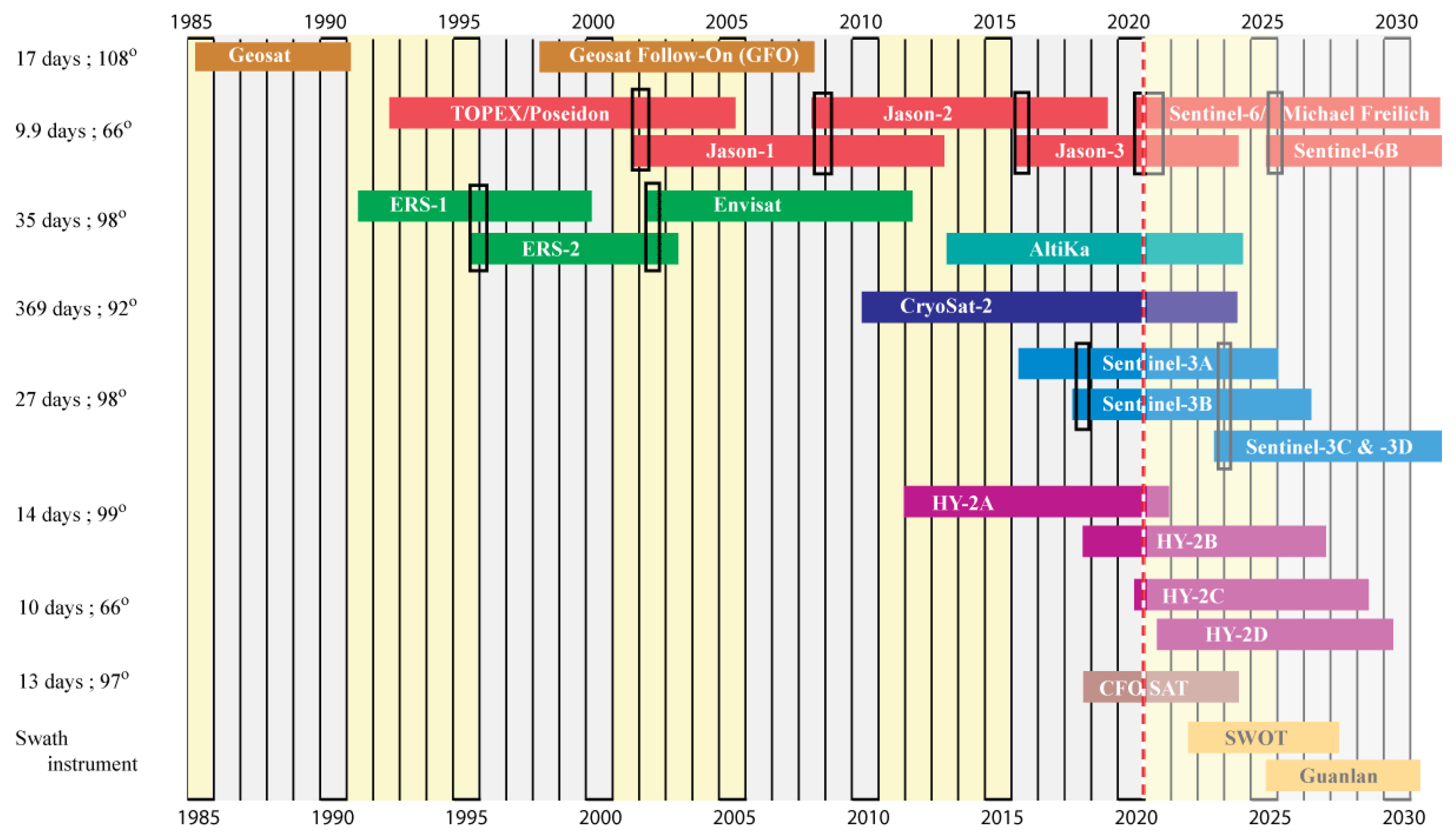
1.1. Long-Term View of Altimetry

Data from the first trials of altimetry on Skylab in 1974 [4], Geos-3 in 1975, and the short-lived Seasat in 1978 [5] enabled NASA to develop documented products over the ocean encompassing sea surface height, wave height and wind speed. With nearly continuous coverage since 1985 (see Figure 1), there are now thousands of oceanographic research papers using altimetry as a trusted data source (http://sealevel.jpl.nasa.gov/science/litdb). These rely on the effort that is spent on the calibration and validation of the data from each individual altimeter. Calibration means assuring the instrument performance conforms to SI (International System of Units) or community accepted standards and to each specific mission requirements. Validation means quantifying the accuracy of the satellite-derived geophysical products [6,7]. The two ideas are referred to together as “cal/val”.
The remainder of this introductory section discusses the scientific requirements on the precision of altimetry measurements and gives an overview of standard cal/val procedures, using both in situ and other satellite measurements. It also provides a perspective on why altimeter data over different surfaces need their own specific cal/val activities, and of how changes in altimeter technology impact these. Section 2 examines the technical developments that support dedicated validation sites, as well as the organizational framework enabling co-ordinated activities. Section 3 then provides a summary of the latest cal/val work in the fields of oceanography, hydrology, cryospheric studies and radiometry. Section 4 details the cal/val issues in moving to swath altimetry, which is the next anticipated advance, with Section 5 providing a brief summary.

1.2. Requirements and Measurements for Marine Cal/Val

The Global Climate Observing System stated that to address questions of climate science the sea level records at scales of 50–100 km should have an accuracy of order 10 mm, with the accuracy of the global average (on a weekly or 10-day basis) being 2–4 mm [8]. To address issues of climate change they stated that the long-term trend of global mean sea level should be known with a stability of 0.3 mm yr 1 . For wave height they put forward an accuracy requirement of 100 mm (but with spatial and temporal resolution beyond the ability of current altimeters [8]). There is no stated requirement on knowledge of the long-term trend in wave height, but Young and Ribal [9] found coherent geographical patterns of order 3 mm yr 1 when combining all altimetric missions from 1985 to 2018.
Altimetric records of sea level can be compared with coastal tide gauges, measurements from offshore platforms, bottom-pressure recorders or surface buoys tied into the space geospatial framework via GNSS (Global Navigation Satellite System) technology. In such exercises, care needs to be taken to account for other atmospheric and oceanic effects (including tides), and land motion, as these may vary between the location and time of the altimeter measurement and those of the reference measurement. Some validation work makes use of many routinely collected sea level measurements, while others focus on one or two dedicated sites, with effort being made to ensure minimal separation in time and space between the satellite and in situ measurements, as well as collecting ancillary data on the atmospheric conditions. Wave height and ocean wind speed data are similarly compared with a large array of metocean buoys. These metocean products are also assessed against numerical models, provided that these assimilate large volumes of calibrated in situ data or have been independently assessed.
Although there are often major cal/val campaigns at the start of a satellite mission, it is also essential that such work continues throughout the lifetime of the spacecraft, because an instrument’s behavior may change due to continued usage and long space exposure. Furthermore, long-term validation series are not only important for reducing the uncertainty in any bias, but also for allowing the estimation of gradual drifts in the altimeter’s measurements. As well as comparison with “ground truth” measurements (which will in themselves have some errors and uncertainties), many studies exploit the potential for inter-satellite comparisons otherwise termed vicarious calibration. Although not an absolute calibration, these efforts help develop the consistency of multi-satellite merged datasets. The European Space Agency’s Climate Change Initiative (CCI) is championing the development of multi-decadal homogenized datasets for 22 different essential climate variables (ECVs), with altimetry contributing strongly to those on sea level [10,11] and wave height [12].

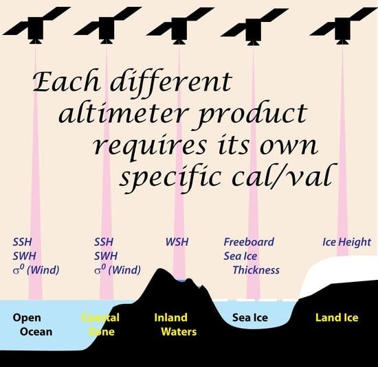
1.3. Altimetry over Non-Marine Surfaces

Although satellite radar altimetry was originally developed for oceanographic studies, by the time of the launch of ERS-1 in 1991, potential applications over other surfaces were being considered. These include land ice, sea ice and inland water surfaces. These surfaces have different topographic and reflective properties from those of the open ocean, leading to different waveform shapes that need their own particular processing and interpretation. This in turn calls for further specialist validation.
Over land ice, the returned echo is a mix of surface and volume scattering, with the proportions dependent upon the moisture content and compactness of the uppermost layer. As these echoes have a more complicated shape, retrackers that fit a predefined shape model are less valid, and instead a robust estimate of range, such as OCOG (offset center-of-gravity) is used. As for sea level and wave height, the construction of multi-satellite climatologies by the Antarctic Ice Sheet CCI [13], requires the minimization of biases and trends between missions to quantify the regions of net loss and gain on that continent. Studies over Arctic sea ice, on the other hand, encounter two distinct types of waveform—one from the surface of the ice and one from the water within leads between the ice [14]. Thus, two different retracking procedures must be implemented, with the property of interest, the freeboard, being the difference of the two. The final domain of interest is inland waters i.e., lakes and rivers. Although ocean retracker solutions may be applied, these are not always appropriate when the reflective surface does not fill the instrument footprint, and the absence of waves may also lead to mirror-like returns. Consequently, over inland waters, different retracking approaches are also evaluated.

1.4. Changes in Altimeter Technology

A further complication in the development of homogeneous time series from altimeter data is the changes in technology used. Although each innovation brings advantages, it also provides challenges in characterizing the differences from previous instruments. AltiKa has been the only instrument to-date operating at Ka-band rather than Ku-band or lower frequencies. This enabled it to operate with a smaller footprint, higher pulse repetition frequency and narrower sample bins in the waveform. However, this meant that its penetration depth within ice was different from preceding instruments. Many preceding altimeters had also operated at S-band or C-band, which are lower frequencies that are less affected by rain than Ku-band, and this allowed the recovery of reliable altimetric data through storms [15]. AltiKa’s operation at a higher frequency means that it is more greatly affected by rain [16] and needs a different model to infer the atmospheric attenuation. Furthermore, a new relationship must be determined linking the backscatter strength ( σ 0 ) to the wind speed [17,18].
Although the early altimeters (up to 2010) only recorded the time variation of the return signal, in a mode now referred to as “Low Resolution Mode” (LRM), CryoSat-2 provided the first spaceborne demonstration of delay-Doppler technology [19]. By recording both the delay and the Doppler shift, it enabled improved along-track resolution of the reflecting points on the Earth’s surface and a better signal to noise ratio through “multi-looking”. Delay-Doppler altimetry, also known as “SAR altimetry” (due to similarity to Synthetic Aperture Radar), has subsequently been implemented on Sentinel-3A (S3A), Sentinel-3B (S3B) and the recently launched Sentinel-6/Michael Freilich (S6MF) satellites. However, the resultant differently shaped waveforms have required a completely new retracking approach [20] and its narrow along-track footprint may affect its ability to measure very long-period swell [21] and may also lead to aliasing effects on the range measurement [22]. Thus, to combine data from different missions requires careful investigations of biases between values from SAR retracking and LRM or PLRM (pseudo-LRM) retracking.
CryoSat-2 also has an interferometric mode, enabling the across-track location of the nearest reflecting surface to be determined. This concept has been greatly extended with plans for future interferometric altimeters (SWOT [23] and Guanlan [24]). These will provide a swath of sea surface topography measurements at fine scales, but will in turn require new validation concepts to assess the precision of the 2-D SSH over 100 km × 100 km scales, and to account for the small, rapid ocean processes contributing to it.
Along with traditional radar altimeters, there have also been examples of altimeters which use lasers for determining the range to the surface, instead. IceSAT and IceSAT-2 [25] are making major contributions over the cryosphere. However, the cal/val challenges over the ocean are very different because their footprint is smaller than the wavelength of typical ocean swell, and they cannot operate through clouds.

2. Cal/Val Procedures

2.1. Facilities, Calibration Sites and Validation Co-Ordination

The main goal of altimetry calibration and validation is to enable altimetry data to be used with confidence globally. One of the key metrics to be assessed is thus the root mean square difference (RMSD). However, estimated RMSD incorporates not only the errors due to altimeter measurement, but also those due to in situ measurement, to the separation in space and time between in situ and altimeter measurements, as well as to the physical mismatch between the two (the altimeter measurement being an almost instantaneous spatial average, with the in situ one being a time average at a fixed point). Disentangling the “altimeter error” from the other ones is often a difficult task. Some of the sources of uncertainty are expected to be near constant or only slowly varying, and these can be assessed by a limited number of well-instrumented sites. Other uncertainties vary with environmental conditions, and a greater understanding is obtained through collating a large amount of validation data spanning the expected range of conditions.
For the limited number of high-precision sites it is essential that there is no spatial or temporal mismatch between the altimeter and the reference measurement. Because of that, these sites are either constructed directly under the planned altimeter flight path, or alternatively, it is the altimeter mission that is specifically designed to overfly these locations. ESA’s first altimeter, ERS-1, flew directly over the Acqua Alta platform near Venice during its initial 3-day mission, whereas NASA/CNES’s TOPEX/Poseidon had the Harvest oil platform off California as its initial cal/val site. Other dedicated sites were then developed off Lampedusa in Italy [26], Senetosa in southwest Corsica [27] and Bass Strait in Australia, and have been used for all subsequent missions in that 10-day orbit. The Bass Strait and Corsica validation sites were subsequently expanded, enabling the assessment of all altimeters occupying the 35-day orbit and, more recently, the 27-day orbits of Sentinel-3 (S3, see Figure 1). The Bass Strait location has been instrumented with an array of moorings and tide gauges. In this special issue, Zhou et al. [28] document recent efforts to understand and minimize the errors associated with using moored GNSS buoys.
A long-standing alternative method of assessing altimeter measurements of range is to use a radar transponder at a precisely known elevation on land, with ESA having invested significantly in dedicated facilities on Crete and Svalbard. (A further site is being developed in Italy that will calibrate the σ 0 measurements too.) Mertikas et al. [29], in this issue, discuss the integration of transponder analysis within the framework of three coastal sites on Crete and Gavdos. The paper details all the ancillary measurement equipment used to link the altimeter record to the actual sea level, and shows that Jason-3, S3A and S3B all have altimeter biases of order 20 mm, thus within their intended performance budgets. Recently, with the increasing use of altimetry for measuring water surface height (WSH) over land water bodies, it has become essential to have range validation sites also representative of those conditions. Lake Issykkul in Kyrgyzstan has been identified as a suitable location, as it is both large and at high altitude (implying that atmospheric path delays are minimal). The site also offers a well-established monitoring station and routine surveys are undertaken with a GNSS-equipped boat. In this special issue, the overview of routine cal/val activities by Quartly et al. [30] provides a comparison of these three different approaches for range validation (Corsica coastal, Crete transponder and Issykkul inland assessment) for the S3A altimeter.
The development of next generation swath altimeters provides a new challenge for cal/val activities, as high-accuracy validation measurements need to be acquired simultaneously over a large area. Yang et al. [31], in this issue, details the development of such a facility off Qingdao in preparation for the launch of China’s wide-swath altimeter, Guanlan. Wang et al. [32] used model simulations to help design the configuration of in situ sensors needed at one of the crossover points for SWOT, the joint US/France/UK/Canada mission due for launch in 2022. The development of new in situ instrumentation to provide high-resolution observations of small-scale rapidly evolving processes is discussed in this issue by Chupin et al. [33]. One shipborne instrument, Cyclopée, can provide a sea level profile to within 0.02 m while travelling at 7 knots (3.6 m s 1 ). The other device, CalNaGeo, is a floating carpet with multiple GNSS receivers towed behind a boat. Nonetheless, many such devices all referenced to the same datum will be required to assess the sea level along-track and across-track gradients within a given satellite swath.
As well as these dedicated sites or focused campaigns, the full assessment of an altimeter’s performance also takes heed of hundreds of routine observations by tide gauges, staging points on rivers and meteorological buoys for the wind and wave fields. The paper by Sánchez-Román et al. [34] in this issue uses the large collection of tide gauges around European coasts to assess the relative accuracy of S3A and Jason-3 altimeters. They compared the 1 Hz data closest to the coast with each of the tide gauges, but found better correlated points (10–15% lower RMSD) typically 7 km further offshore. Furthermore, the agencies aiming to deliver consistent high-accuracy data take notice of input from hundreds of scientists through fora such as the Ocean Surface Topography Science Team (OSTST) and the Sentinel-3 Validation Team (S3VT). This is augmented by routine monitoring after each cycle provided by AVISO (Archivage, Validation et Interprétation des données des Satellites Océanographiques) for the Jason-class satellites and by the Sentinel-3 Mission Performance Centre (S3MPC) for S3A and S3B, with Quartly et al. [30] in this issue describing their work on assessing trends, precision and accuracy over all surfaces.

2.2. Vicarious Calibration

Comparisons with traceable standards are essential for an accurate calibration, especially with concerns about possible trends within datasets. However, a given instrument may only provide a few overflights per year over a dedicated site, especially when in long-period repeat cycles. Furthermore, in situ observations for those comparisons are usually from sheltered coastal conditions. A far greater number of matchups can be garnered by comparison with other satellite data, if these are known to have a clear calibration trail. There may be thousands of these “vicarious calibrations” per year, usually with a near global spread and over a wide range of environmental conditions. This is commonly done for microwave radiometers, using the network of SSM/I sensors as a reference as well as with records of wave height and wind speed. Such intercalibration is critical for the development of homogeneous climatologies incorporating data from several concurrent missions. Within altimetry there has been a major effort to intercalibrate successive sensors in a series by operating a ”tandem mission”, during which a satellite and its immediate successor fly very close together for a few months making the same measurements at minimal temporal lag. ERS-2 followed the track of ERS-1 exactly one day later, with the oceanographic signal assumed to have varied little in that time (although tides and atmospheric corrections will have evolved). Subsequent tandem missions (see Figure 1) have involved altimeters observing the same locations at temporal separations of less than an hour—sometimes only a minute apart—so that changes in atmospheric and tidal conditions are also minimized [35].

3. Cal/Val of Specific Altimeter Products

3.1. Assessment of Wind Speed and Wave Height

Altimetric estimates of wind speed and wave height are frequently assessed in terms of RMSD relative to in situ data from metocean buoys. In some cases, this diagnostic may be dominated by the uncertainties in the buoy measurements as well as the buoy spatial separation from the satellite records. Therefore, researchers have developed procedures to minimize such errors by only employing well-documented consistent datasets and by discarding measurements near the coast, since that region is characterized by higher spatial variability than the open ocean, due to the influence of bottom and lateral boundaries on ocean dynamics. Such practices can then allow some intercomparison between altimeters and in situ observation to assess the performance of different algorithms and/or different altimeters and to monitor their evolution over time.
In this issue, Jiang [36] used four different buoy datasets to assess S3A, S3B and Jason-3 observations. Because of his chosen match-up constraints, slightly different subsets of buoys were used for each altimeter and at different times. They found that Jason-3 gave slightly better accuracy for wave height than S3A and S3B, but that the Sentinels were slightly more accurate for wind speed, which was confirmed by their use of scatterometer data. Section 3 of Quartly et al. [30], in this issue, shows comparisons of S3A SWH and wind speed data with both buoys and models. While numerical models do not provide an absolute reference, they enable quick global assessments to indicate regional patterns of bias in SWH. Such analysis highlighted that S3 SWH is positively biased in regions and seasons of high wave height. The same study also noted that S3A’s PLRM estimates show a greater consistency with those from Jason-3 than do the SAR-derived values.
In this issue, Jia et al. [37] assess the performance of HY-2B by first comparing the precision (noise level) of its estimates with those from Jason-2 and Jason-3. They find that cycle-averages of σ 0 and SWH from the different instruments usually agree to within 0.1 dB and 0.1 m respectively, and that the derived wind data at dual-satellite crossovers agree to within 1 m s 1 . Wang et al. [38], in this issue, also assessed the metocean data from HY-2B, deriving RMSD of 1.10 m s 1 and 0.27 m for the wind speed and SWH values in the standard product. They also apply a “Deep Learning” technique to incorporate the metocean information contained within other fields, and show that algorithms using altimetric wind speed, SWH and standard deviation of σ 0 can reduce the errors to 0.69 m s 1 and 0.20 m, respectively. However, they caution on the danger of over-fitting a complex algorithm when there are not large volumes of independent ground truth data to assess its performance.
Other researchers have assessed new retracking algorithms by applying them to the same altimeter waveform data as used for standard products, thus enabling a relative assessment via the same set of buoys. This has been of particular interest in the coastal zone, where new algorithms are required to deal with known coastal artefacts. Ichikawa et al. [39], in this issue, have looked at a new wave height algorithm for Jason-2, focusing particularly on its performance in regions of low wave height and potential land contamination of the waveforms. Working within the framework of the Sea State CCI, Schlembach et al. [40], in this issue, provided a thorough comparison of several novel SWH algorithms for both S3A and Jason-3. They assessed noise levels of the estimates by considering short-scale variability and compared the many algorithms to both model and buoy data, looking separately at open ocean and coastal conditions. Quartly and Kurekin [41], also in this issue, revisited some of the assumptions in that previous work, showing that the magnitude of errors could be significantly reduced by further constraints on the selection of altimeter data and suitable buoys, and that such a choice would affect the relative ranking of different algorithms. The particular focus on the coastal regime had been the aim of an earlier paper by Nencioli and Quartly [42], who had demonstrated the greater accuracy achieved by S3A’s SAR mode within 15 km of the coast. Their investigation had used model reanalysis output to define maritime regions that would vary coherently with the buoy locations, showing that sometimes close locations would not be expected to agree because of the different exposure of the sites to long-period swell. Jiang [36], in this issue, provided a variant on this approach in that he used that instantaneous spatial variation of SWH in the model to adjust the altimeter value to what should be expected at the buoy location.

3.2. Hydrology Cal/Val

Over the last decade, calibration and validation activities over inland waters have been necessary for the accurate monitoring of water levels in lakes, rivers and reservoirs. For river systems, in situ water level gauges or permanent GNSS receivers situated close to satellite altimetry repeat tracks provide altimetric “virtual stations” and have been widely used for calibration and validation. Along and across-river towed GNSS sections can also be performed, often timed to coincide with satellite overpasses, for local high-resolution calibration. Many lakes have also been equipped with permanent GNSS receivers or water level gauges near satellite overpasses, or benefitted from particular ship-based validation campaigns along satellite tracks crossing the lakes.
Compared with ocean cal/val sites, rivers and lakes can provide an alternative and complementary way of assessing the precision of altimetric measurements and, for example, the range biases associated with particular retrackers. In particular, many ocean correction terms (such as the inverse barometer, the ocean tide, the dynamic atmosphere-induced variability and the sea-state bias) are almost negligible over inland waters. More easily accessible inland water cal/val sites can offer a cheaper opportunity to further increase the density of such activities over the globe. For example, in a large-scale study over more than 100 lakes in the US and Canada, Nielsen et al. [43], in this issue, compare in situ gauges with S3 lake level variations, estimated using different physical and empirical retrackers. They find that the reconstruction of the lake level variations based on the S3 empirical retracker is significantly better compared with that of the physical retracker in terms of the RMSD and correlation. However, the statistics for the Canadian sites show a worse performance in winter due to lake ice cover impacting on the correct mapping of lake levels. Cal/val activities have also been performed over decades from several altimeter missions (TOPEX/Poseidon, Jason-1, Jason-2, Jason-3, GFO, Envisat, Saral/AltiKa and Sentinel-3A) at the long-term calibration site on Lake Issykul [44]. Section 7.1 of Quartly et al. [30], in this issue, covers recent S3 cal/val campaigns there, estimating the altimeter biases for different retrackers against ship-based GNSS data along those satellite tracks.
The detection of river and lake levels in regions of steep surrounding topography or under vegetation is a difficult issue that varies with the altimeter technology. Section 7.3 of the afore-mentioned paper compares the performance of the Sentinel-3 ocean retracker and OCOG for various lakes and reservoirs in the Ebro River basin on the southern flank of the Pyrenees. They found RMSD to be between 0.43 m and 3.6 m depending on topography and proximity of track to gauge. To more precisely position the receiving window and better track the backscattered signal over inland water targets, Sentinel-3 has explored using a priori digital elevation models with open-loop tracking. In this issue, Taburet et al. [45] showed that for the Level-3 S3 products, using this open-loop tracking mode increased the number of water bodies with valid water surface heights by 25% compared with the conventional closed-loop tracking, and this may be further improved to 30% by a recent update to the on-board database. With the future SWOT mission using SAR-interferometry techniques over two 50 km wide swaths to be launched in 2022, we expect to advance on a global inventory of all terrestrial water bodies (lakes, reservoirs, wetlands) whose surface area exceeds 250 m by 250 m and rivers whose width exceeds 100 m at sub-monthly, seasonal, and annual time scales. With the combination of SWOT and along-track altimetry monitoring, we are heading towards a more precise measurement of the global storage change in freshwater bodies and the global change in river discharge, but there are also further challenges in calibrating and validating these 2-D water level surfaces (see Section 4).

3.3. Assessment over Ice Surfaces

While the radar returns over the ocean usually have a very consistent shape (apart from within the coastal zone), the echoes received from land ice, sea ice and the leads within the ice have more complex and varied shapes. For Arctic Ocean altimetry some of the key issues involve classification of the surface giving the returns (sea ice or leads or open ocean), and fitting a waveform model appropriate to each surface. Also, the critical environmental variable of interest is sea-ice thickness, so corrections are needed for variable ice density and the depth of overlaying snow [14]. Given the challenging nature of the environment there is a paucity of “ground truth” data and these are not fully representative of the seasonal variation in properties throughout the freeze/thaw cycle of the marginal ice zone.
Altimetry provides key monitoring information about the ice sheets over Antarctica and Greenland. However, as the echo shape is different again from that over oceans and sea ice, detailed work is still required to determine exactly which portion of the waveform corresponds to the mean range to the surface. This is complicated by seasonal variations in compactness and moisture content of the snow overlaying the ice, leading to changes in penetration depth (which, furthermore, also varies with the radar wavelength employed [46]). Finally, an additional complication comes from determining which part of the ice surface is responsible for the given radar returns, since the point of closest approach can be far from nadir over surfaces with significant slope (i.e., >1°).
NASA’s Operation IceBridge, a decade-long campaign of coincident flights by research aircraft to fill the gap between ICESat and ICESat-2 missions, provides an important contribution to both sea ice and land ice studies, but it does not obviate the need for in situ measurements too. In the current special issue, the only paper covering validation in the cryosphere is Quartly et al. [30], but this does detail the work performed for Sentinel-3A over both land and sea ice. A focus on the very flat topography of Lake Vostok in Antarctica showed RMSD crossovers of 0.08 m, but this value exceeded 1 m when the surface slope was greater than 0.3°. S3A was shown to be unbiased with respect to ICESat-2 which records the height of the ice surface only, whereas the reflections from Cryosat-2 showed a bias of ∼0.26 m deeper, most likely because they are more affected by volume scattering. Regarding sea ice, the afore-mentioned paper only showed that the waveform classification between Cryosat-2 and S3A is consistent and that the inferred ice freeboard measurements from these satellites agreed with one another provided consistent retrackers were used.

3.4. Microwave Radiometers

Microwave Radiometers (MWR) on-board satellite topography missions are combined with the altimeter to correct the altimeter range for the excess path delay resulting from the presence of water vapor in the troposphere. MWR data can also be used to monitor atmospheric characteristics in the troposphere and to constrain operational weather models. The wet path delay (WPD) ranges from a few centimeters to ∼0.5 m and varies spatially and temporally with a correlation radius and time of the order of 30–80 km and of 1 h, respectively. Despite strong improvements in recent years, these small-scale spatial and temporal variations are still not correctly represented by Numerical Weather Prediction (NWP) models, so MWR measurements are essential for accurate WPD corrections. The long-term stability of radiometers on-board altimetry missions is also critical to reduce the uncertainty in the global mean sea level trend, which is a key climate data record. The Sentinel-6 Michael Freilich mission has a requirement to measure the trend in global mean sea level with an uncertainty not exceeding 1 mm yr 1 . On the MWR instrument, this leads to a stability requirement of 0.7 mm yr 1 , which makes the accurate calibration of this instrument critical on a long-term basis.
An MWR designed for providing the necessary altimeter corrections must have a channel close to the water vapor absorption line at 22.235 GHz, and a second around 36.5 GHz sensitive to liquid water found within clouds. The instruments on the TOPEX/Jason satellite series had a third channel around 18.7 GHz that enables the effect of wind roughening of the surface to be mitigated, thereby achieving a better accuracy in WPD estimates. The calibration of an MWR involves monitoring of both internal parameters and external reference targets. In this special issue, Quartly et al. [30] detailed the regular monitoring of the on-board reference temperatures and gain factors for Sentinel-3’s two MWR channels (23.8 and 36.5 GHz), while Frery et al. [47], also in this issue, analyze the performance through vicarious calibration over specific areas (Amazon Forest and cold ocean). This latter paper also applies double-difference methods at crossovers, and a specific processing is performed to enable use of the tandem flight data. They demonstrated that the in-flight calibration of a single instrument is key to achieving the expected performance and that in the context of a constellation (Jason-3 with Sentinel-6MF or S3A with S3B), the intercalibration is even more important. Furthermore, their analysis shows that S3A is well calibrated, consistent with other instruments, and that S3B is calibrated within 0.4 K of S3A.
Picard et al. [48], in this issue, proposed a new method based on the data acquired during the tandem flight between S3A and S3B missions. In this method, they focus on the required harmonization of the sensors and processing algorithms to ensure a seamless continuity between one mission and the other. Applying this approach, they can strongly reduce the bias between the two radiometers for both channels (∼0.5 K) and the standard deviation of the difference (0.3 K).

4. Challenges for Swath Altimetry

The spatial resolution of future wide-swath altimetry missions, including SWOT [49] and Guanlan [24] and possibly others is expected to reach 10–40 km in wavelength, depending on sea-state conditions [32]. These missions offer a real opportunity to detect the anisotropic structure of small mesoscale and submesoscale eddies globally. However, due to insufficient temporal sampling and instrument errors, numerous ocean eddies will remain unobserved. The simulation results of Ma et al. [50] showed that 34% (40%) of coherent eddies cannot be observed by SWOT in the Kuroshio Extension (South China Sea) region, even without considering the effect of internal tides. Both eddy dynamics (motions in geostrophic balance with the surface height difference) and internal gravity waves/tides (unbalanced motion) contribute significantly to the sea surface height, and the relative strength of balanced and unbalanced motion varies geographically and in time [49]. The spatial scale where balanced motion spectral energy exceeds that of the unbalanced motions is the so-called “transition scale” [51]. For all altimetry observations, either 1-D along-track or with 2-D swath observations, the eddies will be very difficult to separate when their spatial scales are smaller than this transition scale.
Centimetric accuracies are required to resolve the smaller mesoscale and submesoscale processes. Several errors of wide-swath altimetry instruments are specific and have not been well estimated, such as baseline roll error, baseline length error, and sea-state bias, etc. These errors will directly limit the accuracy of SSH measurement, so advanced de-noising techniques are required. Dibarboure et al. [52] used an empirical cross-calibration technique to estimate and then remove two spatially coherent errors including baseline roll and length errors. In this issue, Gómez-Navarro et al. [53] propose a method to eliminate the random small-scale noise by optimizing the first to third order derivatives of the SSH in a variational framework. This promising technique was developed and tuned for one region in the western Mediterranean Sea, and for specific wave conditions. To maintain the high spatial resolution of wide-swath altimetry, for SSH and its spatial derivatives of velocity and vorticity, it is critical to develop effective de-noising software for different error conditions for the coming swath altimetry missions.
Compared with cal/val for nadir altimetry, wide-swath altimetry faces new challenges. The first is how to validate the small-scale, rapidly evolving SSH over the width of the swath for a satellite flying at 7 km s 1 , with independent two-dimensional synoptic observations. Secondly, given the improved resolution of the swath observations down to 15 km, validating the SSH variability at the scales of 15–1000 km is also a key challenge [54]. For the larger scales (100–1000 km), we will rely on the large number of nadir altimeter sections that are collocated within a swath. For the scales from 15–100 km, new techniques must be developed. For example, rather than depend on single-point cal/val sites to estimate biases for nadir altimetry, a series of GNSS buoys can be used to monitor biases and trends along-track, or be positioned in 2-D across a swath [28]. By analyzing the potential performance of gliders, moorings and other equipment, Wang et al. [32] proposed an SSH cal/val method based on wavenumber spectral analysis of in situ steric height. In particular, they showed that most of the SSH variability at scales of 20–100 km was captured in the upper 500 m, which can be sampled more rapidly than a full-depth in situ requirement. Zhang et al. [55] further explored the consistency of steric height and SSH by investigating along-track altimetry data and synoptic in situ Argo profiles. Based on the experiment of airborne interferometric altimeter, Yang et al. [31] used GNSS to validate the 2-D SSH variability synoptically in a coastal sea. Finally, an international series of dedicated in situ observations is being planned during the early phases of SWOT, targeting the small-scale dynamics in different regions and seasons and under different SWOT error conditions [56]. Key components of this are to develop and share ideas on new instruments spanning the 20–100 km range, and developing rapid adaptive sampling techniques, and even new analysis techniques for cal/val. This new 2-D observation range of 20–100 km wavelength clearly brings new challenges and opportunities for altimetric cal/val.

5. Summary

Although altimeter data are critical for global observations of many essential climate variables, they can only be used quantitatively for long-term studies of climate change if they are accurately calibrated. This requires (i) that all missions be individually assessed or intercalibrated through comparison with synoptic missions, (ii) that calibration be a mission-long process to address issues of instrumental drift, and (iii) that the altimeter corrections (e.g., from the on-board MWR) also be assessed. Furthermore, as altimetry is now routinely used over a range of surfaces (ocean, rivers, lakes, sea ice and land ice) that return differently shaped waveforms, it is essential that cal/val is performed over each domain using the appropriate retrackers. Over the decades there have been changes in altimeter technology, and also advances in the means to assess them, with developments, for example, in radar transponders and novel GNSS-equipped devices. As always, these large multi-national altimeter missions benefit from a world-wide coterie of scientists performing global analyses or making dedicated local measurements and sharing their results and data to enable a consensus to be developed. With the recent launch of Sentinel-6MF (Figure 2), the fifth satellite in the TOPEX/Jason “reference” orbit, the work of these researchers is as critical as ever for linking data from many missions (see Figure 1) so that concerns about long-term changes can be addressed with confidence.

Author Contributions

Conceptualization, G.D.Q.; editorial oversight of papers in special issue, G.D.Q., G.C., F.N., R.M. and N.P.; writing—original draft preparation, G.D.Q., G.C., F.N., R.M. and N.P.; writing—review and editing, G.D.Q., G.C., F.N., R.M. and N.P.; visualization, G.D.Q. All authors have read and agreed to the published version of the manuscript.

Funding

G.D.Q.’s time was supported by ESA through the Sentinel-3 Mission Performance Centre (Contract No. 4000111836/14/I-LG). G.C. was supported by Natural Science Foundation of China (Contract No. 42030406).

Acknowledgments

We thank the assistant editor for her guidance through the editorial process, and we are also grateful to those who have stepped in to oversee the review process for papers that were written by the Guest Editors of their close scientific colleagues. We also appreciate the detailed feedback provided by Jamie Shutler, Meric Srokosz and Paolo Cipollini plus three additional anonymous referees.

Conflicts of Interest

The authors declare no conflict of interest.

References

  1. Fu, L.L.; Cazenave, A. Satellite Altimetry and Earth Sciences; Academic Press: San Diego, CA, USA, 2001. [Google Scholar]
  2. Brown, G. The average impulse response of a rough surface and its applications. IEEE Trans. Antennas Propag. 1977, 25, 67–74. [Google Scholar] [CrossRef]
  3. Hayne, G. Radar altimeter mean return waveforms from near-normal-incidence ocean surface scattering. IEEE Trans. Antennas Propag. 1980, 28, 687–692. [Google Scholar] [CrossRef] [Green Version]
  4. Vonbun, F.; Marsh, J.G.; McGoogan, J.; Leitao, C.; Vincent, S.; Wells, W. Skylab Earth resources experiment package /EREP/—Sea surface topography experiment. J. Spacecr. Rocket. 1976, 13, 248–250. [Google Scholar] [CrossRef]
  5. Tapley, B.D.; Born, G.H.; Hagar, H.H.; Lorell, J.; Parke, M.E.; Diamante, J.M.; Douglas, B.C.; Goad, C.C.; Kolemkiewicz, R.; Marsh, J.G.; et al. Seasat altimeter calibration: Initial results. Science 1979, 204, 1410–1412. [Google Scholar] [CrossRef] [PubMed]
  6. Justice, C.; Belward, A.; Morisette, J.; Lewis, P.; Privette, J.; Baret, F. Developments in the ‘validation’ of satellite sensor products for the study of the land surface. Int. J. Remote Sens. 2000, 21, 3383–3390. [Google Scholar] [CrossRef]
  7. Sterckx, S.; Brown, I.; Kääb, A.; Krol, M.; Morrow, R.; Veefkind, P.; Boersma, K.F.; Mazière, M.D.; Fox, N.; Thorne, P. Towards a European Cal/Val service for Earth observation. Int. J. Remote Sens. 2020, 41, 4496–4511. [Google Scholar] [CrossRef]
  8. GCOS. Systematic Observation Requirements for Satellite-Based Data Products for Climate. 2011 Update; GCOS-154, Technical Report; GCOS: Geneva, Switzerland, 2011; Available online: https://library.wmo.int/doc_num.php?explnum_id=3710 (accessed on 23 December 2020).
  9. Young, I.R.; Ribal, A. Multiplatform evaluation of global trends in wind speed and wave height. Science 2019, 364, 548–552. [Google Scholar] [CrossRef]
  10. Quartly, G.D.; Legeais, J.F.; Ablain, M.; Zawadzki, L.; Fernandes, M.J.; Rudenko, S.; Carrère, L.; García, P.N.; Cipollini, P.; Andersen, O.B.; et al. A new phase in the production of quality-controlled sea level data. Earth Syst. Sci. Data 2017, 9, 557–572. [Google Scholar] [CrossRef] [Green Version]
  11. Legeais, J.F.; Ablain, M.; Zawadzki, L.; Zuo, H.; Johannessen, J.A.; Scharffenberg, M.G.; Fenoglio-Marc, L.; Fernandes, M.J.; Andersen, O.B.; Rudenko, S.; et al. An improved and homogeneous altimeter sea level record from the ESA Climate Change Initiative. Earth Syst. Sci. Data 2018, 10, 281–301. [Google Scholar] [CrossRef] [Green Version]
  12. Dodet, G.; Piolle, J.F.; Quilfen, Y.; Abdalla, S.; Accensi, M.; Ardhuin, F.; Ash, E.; Bidlot, J.R.; Gommenginger, C.; Marechal, G.; et al. The sea state CCI dataset v1: Towards a sea state climate data record based on satellite observations. Earth Syst. Sci. Data 2020, 12, 1929–1951. [Google Scholar] [CrossRef]
  13. Shepherd, A.; Gilbert, L.; Muir, A.S.; Konrad, H.; McMillan, M.; Slater, T.; Briggs, K.H.; Sundal, A.V.; Hogg, A.E.; Engdahl, M.E. Trends in Antarctic ice sheet elevation and mass. Geophys. Res. Lett. 2019, 46, 8174–8183. [Google Scholar] [CrossRef] [Green Version]
  14. Quartly, G.D.; Rinne, E.; Passaro, M.; Andersen, O.B.; Dinardo, S.; Fleury, S.; Guillot, A.; Hendricks, S.; Kurekin, A.A.; Müller, F.L.; et al. Retrieving sea level and freeboard in the Arctic: A review of current radar altimetry methodologies and future perspectives. Remote Sens. 2019, 11, 881. [Google Scholar] [CrossRef] [Green Version]
  15. Quartly, G. Achieving accurate altimetry across storms: Improved wind and wave estimates from C Band. J. Atmos. Ocean. Technol. 1997, 14, 705–715. [Google Scholar] [CrossRef]
  16. Tournadre, J.; Lambin-Artru, J.; Steunou, N. Cloud and rain effects on AltiKa/SARAL Ka-band radar altimeter—Part I: Modeling and mean annual data availability. IEEE Trans. Geosci. Remote Sens. 2009, 47, 1806–1817. [Google Scholar] [CrossRef] [Green Version]
  17. Lillibridge, J.; Scharroo, R.; Abdalla, S.; Vandemark, D. One- and two-dimensional wind speed models for Ka-band altimetry. J. Atmos. Ocean. Technol. 2014, 31, 630–638. [Google Scholar] [CrossRef]
  18. Quartly, G.D. Metocean comparisons of Jason-2 and AltiKa—A method to develop a new wind speed algorithm. Mar. Geod. 2015, 38, 437–448. [Google Scholar] [CrossRef]
  19. Raney, R.K. The delay/Doppler radar altimeter. IEEE Trans. Geosci. Remote Sens. 1998, 36, 1578–1588. [Google Scholar] [CrossRef]
  20. Ray, C.; Martin-Puig, C.; Clarizia, M.P.; Ruffini, G.; Dinardo, S.; Gommenginger, C.; Benveniste, J. SAR altimeter backscattered waveform model. IEEE Trans. Geosci. Remote Sens. 2015, 53, 911–919. [Google Scholar] [CrossRef]
  21. Moreau, T.; Tran, N.; Aublanc, J.; Tison, C.; Le Gac, S.; Boy, F. Impact of long ocean waves on wave height retrieval from SAR altimetry data. Adv. Space Res. 2018, 62, 1434–1444. [Google Scholar] [CrossRef]
  22. Reale, F.; Dentale, F.; Carratelli, E.P.; Fenoglio-Marc, L. Influence of sea state on sea surface height oscillation from Doppler altimeter measurements in the North Sea. Remote Sens. 2018, 10, 1100. [Google Scholar] [CrossRef] [Green Version]
  23. Durand, M.; Fu, L.; Lettenmaier, D.P.; Alsdorf, D.E.; Rodriguez, E.; Esteban-Fernandez, D. The Surface Water and Ocean Topography mission: Observing terrestrial surface water and oceanic submesoscale eddies. Proc. IEEE 2010, 98, 766–779. [Google Scholar] [CrossRef]
  24. Chen, G.; Tang, J.; Zhao, C.; Wu, S.; Yu, F.; Ma, C.; Xu, Y.; Chen, W.; Zhang, Y.; Liu, J.; et al. Concept design of the “Guanlan” science mission: China’s novel contribution to space oceanography. Front. Mar. Sci. 2019, 6, 194. [Google Scholar] [CrossRef] [Green Version]
  25. Markus, T.; Neumann, T.; Martino, A.; Abdalati, W.; Brunt, K.; Csatho, B.; Farrell, S.; Fricker, H.; Gardner, A.; Harding, D.; et al. The Ice, Cloud, and land Elevation Satellite-2 (ICESat-2): Science requirements, concept, and implementation. Remote Sens. Environ. 2017, 190, 260–273. [Google Scholar] [CrossRef]
  26. Ménard, Y.; Jeansou, E.; Vincent, P. Calibration of the TOPEX/POSEIDON altimeters at Lampedusa: Additional results at Harvest. J. Geophys. Res. Ocean. 1994, 99, 24487–24504. [Google Scholar] [CrossRef]
  27. Bonnefond, P.; Exertier, P.; Laurain, O.; Guinle, T.; Féménias, P. Corsica: A 20-Yr multi-mission absolute altimeter calibration site. Adv. Space Res. 2019. [Google Scholar] [CrossRef]
  28. Zhou, B.; Watson, C.; Legresy, B.; King, M.A.; Beardsley, J.; Deane, A. GNSS/INS-equipped buoys for altimetry validation: Lessons learnt and new directions from the Bass Strait Validation Facility. Remote Sens. 2020, 12, 3001. [Google Scholar] [CrossRef]
  29. Mertikas, S.; Tripolitsiotis, A.; Donlon, C.; Mavrocordatos, C.; Féménias, P.; Borde, F.; Frantzis, X.; Kokolakis, C.; Guinle, T.; Vergos, G.; et al. The ESA Permanent Facility for altimetry calibration: Monitoring performance of radar altimeters for Sentinel-3A, Sentinel-3B and Jason-3 using transponder and sea-surface calibrations with FRM standards. Remote Sens. 2020, 12, 2642. [Google Scholar] [CrossRef]
  30. Quartly, G.D.; Nencioli, F.; Raynal, M.; Bonnefond, P.; Nilo Garcia, P.; Garcia-Mondéjar, A.; Flores de la Cruz, A.; Crétaux, J.F.; Taburet, N.; Frery, M.L.; et al. The roles of the S3MPC: Monitoring, validation and evolution of Sentinel-3 altimetry observations. Remote Sens. 2020, 12, 1763. [Google Scholar] [CrossRef]
  31. Yang, L.; Xu, Y.; Zhou, X.; Zhu, L.; Jiang, Q.; Sun, H.; Chen, G.; Wang, P.; Mertikas, S.P.; Fu, Y.; et al. Calibration of an airborne interferometric radar altimeter over the Qingdao coast sea, China. Remote Sens. 2020, 12, 1651. [Google Scholar] [CrossRef]
  32. Wang, J.; Fu, L.L.; Qiu, B.; Menemenlis, D.; Farrar, J.T.; Chao, Y.; Thompson, A.F.; Flexas, M.M. An observing system simulation experiment for the calibration and validation of the Surface Water Ocean Topography sea surface height measurement using in situ platforms. J. Atmos. Ocean. Technol. 2018, 35, 281–297. [Google Scholar] [CrossRef]
  33. Chupin, C.; Ballu, V.; Testut, L.; Tranchant, Y.T.; Calzas, M.; Poirier, E.; Coulombier, T.; Laurain, O.; Bonnefond, P.; FOAM Project Team. Mapping sea surface height using new concepts of kinematic GNSS instruments. Remote Sens. 2020, 12, 2656. [Google Scholar] [CrossRef]
  34. Sánchez-Román, A.; Pascual, A.; Pujol, M.I.; Taburet, G.; Marcos, M.; Faugère, Y. Assessment of DUACS Sentinel-3A altimetry data in the coastal band of the European Seas: Comparison with tide gauge measurements. Remote Sens. 2020, 12, 3970. [Google Scholar] [CrossRef]
  35. Clerc, S.; Donlon, C.; Borde, F.; Lamquin, N.; Hunt, S.E.; Smith, D.; McMillan, M.; Mittaz, J.; Woolliams, E.; Hammond, M.; et al. Benefits and lessons learned from the Sentinel-3 tandem phase. Remote Sens. 2020, 12, 2668. [Google Scholar] [CrossRef]
  36. Jiang, H. Indirect validation of ocean remote sensing data via numerical model: An example of wave heights from altimeter. Remote Sens. 2020, 12, 2627. [Google Scholar] [CrossRef]
  37. Jia, Y.; Yang, J.; Lin, M.; Zhang, Y.; Ma, C.; Fan, C. Global assessments of the HY-2B measurements and cross-calibrations with Jason-3. Remote Sens. 2020, 12, 2470. [Google Scholar] [CrossRef]
  38. Wang, J.; Aouf, L.; Jia, Y.; Zhang, Y. Validation and calibration of significant wave height and wind speed retrievals from HY2B altimeter based on Deep Learning. Remote Sens. 2020, 12, 2858. [Google Scholar] [CrossRef]
  39. Ichikawa, K.; Wang, X.F.; Tamura, H. Capability of Jason-2 subwaveform retrackers for significant wave height in the calm semi-enclosed Celebes Sea. Remote Sens. 2020, 12, 3367. [Google Scholar] [CrossRef]
  40. Schlembach, F.; Passaro, M.; Quartly, G.D.; Kurekin, A.; Nencioli, F.; Dodet, G.; Piollé, J.F.; Ardhuin, F.; Bidlot, J.; Schwatke, C.; et al. Round Robin assessment of radar altimeter Low Resolution Mode and Delay-Doppler retracking algorithms for significant wave height. Remote Sens. 2020, 12, 1254. [Google Scholar] [CrossRef] [Green Version]
  41. Quartly, G.D.; Kurekin, A.A. Sensitivity of altimeter wave height assessment to data selection. Remote Sens. 2020, 12, 2608. [Google Scholar] [CrossRef]
  42. Nencioli, F.; Quartly, G.D. Evaluation of Sentinel-3A wave height observations near the coast of southwest England. Remote Sens. 2019, 11, 2998. [Google Scholar] [CrossRef] [Green Version]
  43. Nielsen, K.; Andersen, O.B.; Ranndal, H. Validation of Sentinel-3A based lake level over US and Canada. Remote Sens. 2020, 12, 2835. [Google Scholar] [CrossRef]
  44. Crétaux, J.F.; Bergé-Nguyen, M.; Calmant, S.; Jamangulova, N.; Satylkanov, R.; Lyard, F.; Perosanz, F.; Verron, J.; Samine Montazem, A.; Le Guilcher, G.; et al. Absolute calibration or validation of the altimeters on the Sentinel-3A and the Jason-3 over Lake Issykkul (Kyrgyzstan). Remote Sens. 2018, 10, 1679. [Google Scholar] [CrossRef] [Green Version]
  45. Taburet, N.; Zawadzki, L.; Vayre, M.; Blumstein, D.; Le Gac, S.; Boy, F.; Raynal, M.; Labroue, S.; Crétaux, J.F.; Femenias, P. S3MPC: Improvement on inland water tracking and water level monitoring from the OLTC onboard Sentinel-3 altimeters. Remote Sens. 2020, 12, 3055. [Google Scholar] [CrossRef]
  46. Lacroix, P.; Dechambre, M.; Legrésy, B.; Blarel, F.; Rémy, F. On the use of the dual-frequency ENVISAT altimeter to determine snowpack properties of the Antarctic ice sheet. Remote Sens. Environ. 2008, 112, 1712–1729. [Google Scholar] [CrossRef]
  47. Frery, M.L.; Siméon, M.; Goldstein, C.; Féménias, P.; Borde, F.; Houpert, A.; Olea Garcia, A. Sentinel-3 microwave radiometers: Instrument description, calibration and geophysical products performances. Remote Sens. 2020, 12, 2590. [Google Scholar] [CrossRef]
  48. Picard, B.; Bennartz, R.; Fell, F.; Frery, M.L.; Siméon, M.; Bordes, F. Assessment of the “zero-bias line” homogenization method for microwave radiometers using Sentinel-3A and Sentinel-3B tandem phase. Remote Sens. 2020, 12, 3154. [Google Scholar] [CrossRef]
  49. Morrow, R.; Fu, L.L.; Ardhuin, F.; Benkiran, M.; Chapron, B.; Cosme, E.; d’Ovidio, F.; Farrar, J.T.; Gille, S.T.; Lapeyre, G.; et al. Global observations of fine-scale ocean surface topography with the Surface Water and Ocean Topography (SWOT) mission. Front. Mar. Sci. 2019, 6, 232. [Google Scholar] [CrossRef]
  50. Ma, C.; Guo, X.; Zhang, H.; Di, J.; Chen, G. An investigation of the influences of SWOT sampling and errors on ocean eddy observation. Remote Sens. 2020, 12, 2682. [Google Scholar] [CrossRef]
  51. Qiu, B.; Chen, S.; Klein, P.; Wang, J.; Torres, H.; Fu, L.L.; Menemenlis, D. Seasonality in transition scale from balanced to unbalanced motions in the world ocean. J. Phys. Oceanogr. 2018, 48, 591–605. [Google Scholar] [CrossRef] [Green Version]
  52. Dibarboure, G.; Labroue, S.; Ablain, M.; Fjortoft, R.; Mallet, A.; Lambin, J.; Souyris, J. Empirical cross-calibration of coherent SWOT errors using external references and the altimetry constellation. IEEE Trans. Geosci. Remote Sens. 2012, 50, 2325–2344. [Google Scholar] [CrossRef]
  53. Gómez-Navarro, L.; Cosme, E.; Sommer, J.L.; Papadakis, N.; Pascual, A. Development of an image de-noising method in preparation for the Surface Water and Ocean Topography satellite mission. Remote Sens. 2020, 12, 734. [Google Scholar] [CrossRef] [Green Version]
  54. Li, Z.; Wang, J.; Fu, L.L. An observing system simulation experiment for ocean state estimation to assess the performance of the SWOT mission: Part 1—A twin experiment. J. Geophys. Res. Ocean. 2019, 124, 4838–4855. [Google Scholar] [CrossRef]
  55. Zhang, Q.; Yu, F.; Chen, G. The difference of sea level variability by steric height and altimetry in the North Pacific. Remote Sens. 2020, 12, 379. [Google Scholar] [CrossRef] [Green Version]
  56. D’Ovidio, F.; Pascual, A.; Wang, J.; Doglioli, A.M.; Jing, Z.; Moreau, S.; Grégori, G.; Swart, S.; Speich, S.; Cyr, F.; et al. Frontiers in fine-scale in situ studies: Opportunities during the SWOT fast sampling phase. Front. Mar. Sci. 2019, 6, 168. [Google Scholar] [CrossRef]
Figure 1. Gantt chart showing the altimetry missions since 1985, classified by their principal orbit (repeat period and inclination), which governs which validation sites are overflown. Investigating long-term trends requires that all the missions used be referenced to the same standard. The black boxes indicate tandem missions when a preceding satellite was used to calibrate a new mission. Note, ERS-1 was in a 3-day orbit for the early part of the mission, Geosat only assumed 17-day repeat after November 1986, while other missions were moved into geodetic phases for the latter years of their missions.
Remotesensing 13 00125 g001
Figure 2. Sentinel-6 Michael Freilich was launched on 21 November 2020 and will be the first to offer fully focused SAR operation over all the ocean between 66°S and 66°N. To achieve a precise intercalibration it will be in a tandem orbit within 30 s of Jason-3 for 12 months. Images courtesy of NASA and ESA.
Remotesensing 13 00125 g002
Publisher’s Note: MDPI stays neutral with regard to jurisdictional claims in published maps and institutional affiliations.

