Abstract
Sentinel-1 synthetic aperture radar (SAR) is one of the most advanced open-access satellite systems available, benefitting from its capability for earth observation under all-weather conditions. In this study, more than 280 Sentinel-1 SAR images are used to derive significant wave heights (Hs) of the sea surface using a polarization-enhanced methodology. Two study areas are selected: one is located near Hawai’i in a deep water region, and the other is in transitional water off the U.S. west coast, where the U.S. National Oceanic and Atmospheric Administration (NOAA) buoy data are available for validations. The enhanced Hs retrieval methodology utilizes dual-polarization SAR image data with strong non-Bragg radar backscattering, resulting in a better estimate of the cut-off wavelength than from those using single-polarization SAR data. The new method to derive Hs is applied to SAR images from 2017 taken from both deep water (near Hawai’i) and coastal water locations (off the U.S. West coast). The assessments of the retrieved Hs from SAR images suggest that the dual-polarization methodology can reduce the estimated Hs RMSE by 24.6% as compared to a single-polarization approach. Long-term reliability of the SAR image-derived Hs products based on the new methodology is also consolidated by large amount of in-situ buoy observations for both the coastal and deep waters.
1. Introduction
Synthetic aperture radar (SAR) systems are capable of observing ocean surface in high spatial resolution under all weather conditions. Over the past 40 years, the potential of using digitally processed SAR images of ocean surfaces has been quantitatively proven to be able to detect multiple wave parameters such as ocean wave direction, wavelength, and wave height [1,2]. Since the launch of Seasat in 1978, Almaz-1 in 1991, and ERS-1 in 1991, a large number of surface imprints of small-, meso-, and sub-synoptic-scales of oceanic and atmospheric phenomena have been investigated using SAR images to explore atmospheric and oceanic dynamics [3,4,5,6,7,8]. Current SAR systems are widely utilized and offer many resolution scales. The C-Band (5.405 GHz) Sentinel-1 SAR is one of the most used systems that generate reliable, open-access, and continuous observations of the ocean surfaces [9,10].
The detection of ocean surface waves by spaceborne SAR is made possible through the mechanisms of (1) the lifting and tilting of Bragg waves by long gravity waves, which can be modulated by the local geometry and slope of the sea surface along the long waves (tilt modulation), (2) the backscatter intensity variation due to the modulation of short gravity waves by longer waves (hydrodynamic modulation/straining), which changes the local roughness, and (3) an azimuthal displacement of the scattering elements in the SAR image caused by the Doppler shift of the return signal, associated with the wave’s orbital velocity (velocity bunching) [3,11]. The existence of ships, oil spills, or rain patches can introduce higher complexity to these mechanisms. When swell-dominated ocean waves are moving approximately in the range direction, the tilt modulation plays an important role in SAR imaging [1,3,12]. As the ocean surface wave propagation deflects from the range direction, the velocity bunching would be a primary modulation in SAR imaging of ocean surface wave [4].
Retrieval algorithms of ocean wave height have been investigated over recent decades, which developed theoretical-based algorithms such as the Max Planck Institute Algorithm (MPI) [13,14], the numerical wave model (WAM; WAMDI group) [15], the semi-parametric algorithm (SPRA) [16], the parameterized first-guess spectrum method (PFSM) [17,18], the partition rescaling and shift algorithm (PARSA) [18], as well as recent fully empirical algorithms for C-band sensors such as CWAVE_ERS for ERS-2 SAR [19], CWAVE_ENVI for Envisat ASAR [20], and CWAVE_S1A for Sentinel-1 SAR [21] which operate without calculating the ocean wave spectrum. In recent methodologies, different strategies are employed to retrieve the significant wave height by using the azimuth cut-off wavelength derived from SAR images. The relative motions between satellite and ocean surface scatterers introduce additional Doppler frequency shifts and reduce its nominal azimuthal resolution by a strong cut-off in the SAR spectra [19,22]. However, the azimuth cut-off wavelength (λco) may also provide additional information about sea state information such as significant wave height (Hs), based on the fact that λco is proportional to the second moment of a wave height spectrum, wind speed [8,11], and wave orbital velocity [23]. Geophysical models are developed to explain the relation between λco and Hs, as well as wind speed (U10) at 10 m above sea level [7]. It has been suggested that λco is correlated with Hs in all sea state conditions, while the correlation with U10 is high only for fully developed sea states [23]. The empirical methodology of estimating Hs from λco for coastal waters was introduced using ERS-1 SAR images [5]. Based on the SAR-derived λco and an empirical relationship between mean and peak periods of ocean waves, a new semi-empirical approach was developed to estimate the significant wave height from Envisat ASAR data based on the theoretical SAR ocean wave imaging mechanism and the empirical relation between two types of wave periods [24,25]. This semi-empirical algorithm has been proven to be robust and flexible, and there have been a number of studies examining the possibilities of estimating Hs from λco by using C-band satellite systems such as ERS-1 SAR [26], Radarsat-2 [27], Envisat ASAR [28,29], Sentinel-1 SAR [8,21,28], and Gaofen-3 SAR [18,30,31,32].
In this paper, we develop a new strategy to estimate the significant wave height, which can enhance the estimation accuracies of the cut-off wavelength and Hs. Our strategy utilizes dual-polarization SAR images and strengthens the observation capability of the SAR platform for estimating ocean surface wave parameters. The methodology is validated by comparing the derived Hs with in-situ buoy measurement data. We then analyzed the seasonal variation of Hs based on satellite SAR derivations in certain areas. The remainder of the paper is organized as follows. Section 2 presents the methodology and data used in the study. Section 3 describes the dual-polarization strategy to derive the dominant wavelength and the cut-off wavelength. Section 4 gives the results and the methodology validation and followed by the discussion in Section 5 and the conclusion in Section 6.
2. Methodology and Data
2.1. Methodology
The general Sentinel-1 SAR imaging geometry can be seen in [33]. In the range direction, the wave imaging process for SAR is the same as that for any real aperture radar (RAR) [2], with an additional range-compression technique based on the Doppler shift that has been used to achieve the high spatial resolution [34]. However, in the azimuthal direction, the SAR observation of the Doppler frequency shift is sensitive to the relative velocity between the radar and the target. More prolonged wave orbital motion has a large component in the azimuthal direction; therefore, it is capable of causing image degradation in the azimuthal direction. This may affect the short wave in the azimuthal direction imaged using SAR. Therefore, a cut-off wavelength is introduced. The cut-off wavelength is linked to the wave’s orbital velocity, and the wave height can be retrieved based on the cut-off wavelength. The mean-square orbital velocity in the range direction, ρvv can be expressed as,
where D(ω, φ) is the normalized directional distribution function, with , where φ is the azimuthal angle, S(ω) is the wave height spectrum, ω is the angular frequency. The range velocity transfer function, , is given by [13],
where θ is the SAR microwave incidence angle. If the directional distribution of waves is narrow and concentrated in a certain direction, substitution of Equation (2) into Equation (1) yields,
and
where , and Ψ is the azimuthal angle of dominant waves determined from the wavenumber spectrum (Ψ = 0° for azimuth propagating waves and Ψ = 90° for range propagating waves). The can be considered nearly constant over the dominant part of wave spectrum, so G(ω) is independent of ω, given by,
with and B = 2.44. Therefore, Equation (3) becomes,
The azimuthal cut-off wavelength, λco is related to the mean-square orbital velocity in the range direction, ρvv by,
where β is the ratio of slant range (R) to velocity (V) of the SAR platform. The azimuthal cut-off wavelength can be derived as,
G is incorporated into Equation (8), compared with the study of Stopa and Mouche [21], reflecting the incidence angle change in a SAR image scene. The significant wave height (Hs) and the mean period of ocean wave (T0) are defined as,
and
Combining Equations (8)–(10), we obtain the relationship among , Hs, and T0:
There is an empirical relation between mean wave period and peak wave period Tp as [25],
Using the dispersion relation of dominant wavelength, λp and Tp for finite water depth [35] are linked by,
where d is the water depth. Therefore, Hs is derived as,
Next, let , so that,
Then, Equation (14) can be changed as,
Equation (16) indicates that if we determine the cut-off wavelength and dominant wavelength from SAR images, the significant wave height can be estimated.
2.2. SAR Dataset and Study Area
This study employs Level-1 Ground Range Detected (GRD) C-Band Sentinel-1A and 1B SAR satellite images, covering the entire year of 2017. The SAR data are publicly accessible and are available at approximately weekly intervals. Sentinel-1A was launched in April 2014 and followed by Sentinel-1B in April 2016, with a 6-day combined revisit period. We used the double (VV + VH) polarized mode in the Level-1 Ground Range detected interferometric wide (IW) mode, with 10 m high-resolution pixel size of multi-look IW mode images. An improved Lee filter of 7 × 7 pixels window size is applied to reduce the speckle noise [36]. The dataset contains three layers of channels, the VV, VH, and incidence angle.
The study areas are located in the waters near Hawai’i for the deep-water scenario and the Channel Islands of the West Coast of the USA for the coastal water scenario. These areas include the U.S. National Data Buoy Center (NDBC) buoy stations of 51000, 51002, 51003, 51004 in the deep-water region, and 46262, 46251, 46219, 46218, 46069, 46054, 46053, and 46025 in the coastal water region. There are 282 SAR imagery scenes available during 2017. Figure 1 shows the regions of interest and Table 1 lists details of the datasets. In-situ measurements of Hs, wind speed at 10 m height above the sea surface (U10), and mean wave direction are collected from the NDBC buoys located inside the boundary of the chosen SAR image scenes. These measurements are used to validate the Hs estimation results from SAR observations. The two closest hourly NDBC buoy data to the SAR acquisition time are selected and averaged as ground truths, and if the SAR acquisition time is within 15 min to either of the two closest hourly NDBC data, the closest measurement is chosen. Surface waves are classified into swells and fetch-limited waves based on the difference between the wind direction and the buoy-measured mean wave direction.
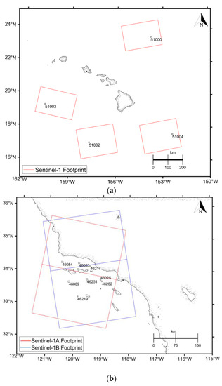
Figure 1.
Regions of interest with Sentinel-1 synthetic aperture radar (SAR) image footprints overlaid as colored boxes in the waters near Hawai’i (a) and near the Channel Islands on the West Coast of the USA (b).

Table 1.
NDBC buoy location, water depth, wave type, and wind speed at 10 m height above the sea surface (U10), as well as the total number of SAR images used.
We assume that if the wind and wave direction difference is higher than 45°, the waves are classified as swells, while the others are defined as the fetch-limited or wind-generated waves. The U10 is also divided into three categories, ≤4 ms−1, 4–10 ms−1, and >10 ms−1 to represent the low, medium and high wind speed environments.
2.3. Data Pre-Processing
Using the SAR imagery to derive the wave parameters via a two-dimensional wave spectrum requires visible and clear wave patterns [19]. Thus, in our study, we use SAR image scenes with visible ocean wave streaks to eliminate the contamination effects of current shears, oil slicks, ships, or islands, leaving only the wave modulation. In addition, high homogeneity SAR images allow better interpretation of the ocean surface signatures. Here, a homogeneity parameter, defined as the normalized mean intensity variance (cvar) is given in [21,37] as,
where ⟨I⟩ is the mean intensity of a scene subset data. In general, scenes with weak ocean wave modulations or dominated by speckle noise will exhibit a normalized mean intensity variance that is closer to unity. The homogeneity of the processed images is maintained by limiting the normalized variance of the VV polarization to the range of 1.1 ≤ cvar ≤ 1.9.
3. Dual-Polarization Enhancement of Wave Spectrum Estimates
3.1. Dual-Polarization Enhancement Processing
The ocean surface radar backscattering consists of two different components, Bragg resonance and non-Bragg resonance scattering [38,39]. For the VV polarization, the Bragg resonant scattering is stronger than the non-Bragg scattering which is basically induced by volume scattering of the wind-induced breaking on the wave crests [40]. Previous studies show that the co-polarization Normalized Radar Cross Section (NRCS) depends on radar incidence angle and wind direction, while the cross-polarization is nearly independent of these parameters but has a linear relationship with ocean surface wind speed [41,42,43].
Under high-wind conditions, Bragg scattering is no longer the only scattering mechanism; imaged features associated with breaking waves such as foam and white caps become more predominant and need to be addressed [44,45,46]. Over rain-free areas, the VH polarization sensitivity at high winds is more than 3.5 times larger than in VV, when the wave breaking effect plays a vital role in the cross-polarized scattering.
As the wind speed increases in a high sea state, the non-Bragg scattering is enhanced substantially. This phenomenon implies that the wave streaks in a cross-polarized image can be enhanced. In the cross-polarized image, the wave streaks, generally, are weaker than those in the co-polarized image, and orbital velocity-induced displacements in the azimuthal direction can also appear in the cross-polarized SAR image. Thus, it is plausible that the composition of the co-polarized and cross-polarized images may reveal stronger signals of the cut-off wavelength than the co-polarized image alone. Based on this, we develop a strategy to derive the dominant wavelength and cut-off wavelength by using the SAR image of composite polarizations (or dual polarization).
It is expected that the combination of the spectra of the VV and VH polarization SAR images enhances cut-off wavelength from the SAR image spectrum. Thus, we define a dual spectrum (DuSP) of VV and VH polarization NRCS as,
where SP represents the spectrum function, and the rB is the ratio of mean VV polarization NRCS to the mean VH polarization NRCS, expressed as,
where the overbar denotes the mean calculation. In this study, the value of rB is calculated by Equation (19), and it is close to 7.3 which is used in Zhang et al.’s estimation [40] with much larger datasets.
3.2. Peak of Dominant Wavelength and Azimuth Cut-off Wavelength
The peak of the dominant wavelength (λp) and the azimuth cut-off wavelength (λco) are obtained from the 2D wave spectrum of the backscattering composite of the two polarizations. The 10 km × 10 km subset size is chosen to minimize the need of using a directional function, by assuming that the wave angular frequency and propagation direction is constant on the entire subset, and reduces the probability of multi-wave occurrence in wind-sea dominant environment. A median filter of 5 × 5 pixels is applied to SAR VV and VH polarization images. This simple filtering can effectively suppress SAR NRCS noise from Rayleigh scattering that contribute less than 50 m [12]. We found that this step is important to improve the estimation of the dominant wavelength from SAR NRCS with multi-waves observed and the wave propagation direction unchanged.
The wave spectra are estimated by applying a 2-dimensional discrete Fast Fourier Transform (2D-DFFT) to the SAR NRCS as follows,
where M and N are the numbers of SAR NRCS in the x and y directions in both spatial and wavenumber domains, respectively; k = (0, 1, 2, …, M−1) and l = (0, 1, 2, ..., N−1). The wavenumber in the x direction (kx) is 2πk/X and the wavenumber in the y direction (ky) is 2πl/Y, in which, X is the spatial scale of the SAR image in the x direction and Y is the spatial scale in the y direction.
The dominant wavelengths (λp) are estimated by using the 2D wavenumber spectrum of the SAR image of the NRCS. This can be done quickly for a single spectrum peak, though for multiple peaks in a wave spectrum, a careful selection of the highest and strongest peak is necessary to determine the dominant wavelength, which is longer than λco since SAR is not able to detect waves with shorter wavelengths than λco. The dominant wavelength peak is calculated by,
Figure 2 shows two VV (a, b) and two VH-polarized (c, d) SAR NRCS and their 2-D wavenumber spectra; one pair of VV and VH images are co-located with NDBC 51000 and the other with NDBC 46054. Each of the images represents a 10 km2 subset. This data can reveal surface wave patterns, although the wave streaks in VH-polarized images (c, d) are a little weak. These wave patterns are also shown in the 2-D wavenumber spectra (e, f, g, h). Based on the 2-D spectra, the composite spectra are derived from Equation (20).
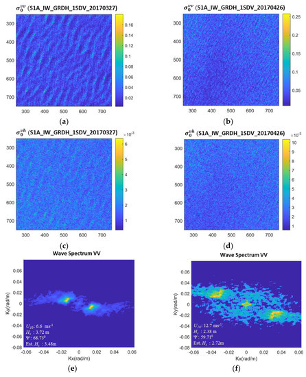
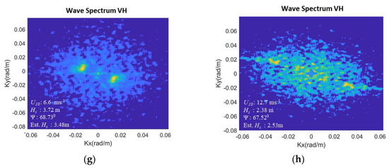
Figure 2.
5 km × 5 km subset taken from the 10 km × 10 km SAR Normalized Radar Cross Section (NRCS) of VV (a) and VH-polarizations (c) on 27 March 2017, co-located with NDBC 51000 and SAR NRCS of VV (b) and VH-polarizations (d) on 26 April 2017, co-located with NDBC 46054. 2-D wave spectrum of the SAR VV (e) and VH (g) NRCS on 27 March 2017, and spectra of the SAR VV (f) and VH (h) NRCS on 26 April 2017.
The spectrum averages over the x-axis (in the range direction) are obtained, as shown in Figure 3 for the VV and VH compositions (c, d), as well as for the VV polarizations (a, b). Based on the polarization-enhanced wave spectra, the dominant wavelength can be characterized by a substantial peak located between 0.06 to 0.015 radm−1 in both the range and azimuth directions, respectively. This spectral peak is identified to determine a reasonable wavelength. However, in coastal cases, we often found high λp on low wave height environments in coastal areas, so in those cases, the secondary peak is selected as an appropriate λp that is less than 0.02 rad m−1.
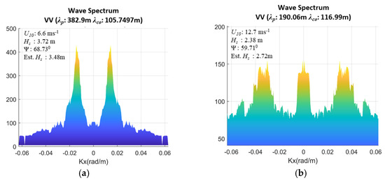
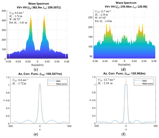
Figure 3.
Averages over the range (x-axis) of the 2-D wavenumber spectra of VV NRCS (a) and composite polarization NRCS (c) on 27 March 2017, and averages over the range (x-axis) of the 2-D wavenumber spectra of VV NRCS (b) and composite polarization NRCS (d) on 26 April 2017, The azimuth correlation functions of the composite polarization NRCS on 27 March 2017 (e) and 26 April 2017 (f).
The azimuthal cut-off wavelength (λco) is the shortest wave that can be detected in the SAR image. It has been found to be highly correlated to Hs studies because of its sensitivity to long waves [47]. The theoretical basis for the azimuth cut-off method is related to the influence of the orbital motion of the surface waves due to the velocity bunching mechanism. As Hs grows higher, additional Doppler shifts distort the phase of the backscattered signal that is used to synthesize the azimuth resolution, resulting in a “low-pass filtered” SAR image in the azimuth direction [48]. λco is computed by fitting a Gaussian function to the azimuthal autocorrelation function (ACF) of the composite wave spectra derived based on Equation (20). ACF is obtained by the inverse fast Fourier transform (IFFT) of the azimuthal section of power spectral density (PSD) [22,49], given by,
where the overbar over DuSP represents the spectrum average over the range direction. A median filter with 5 × 5 size window is then applied to the resulting ACF to remove speckle noise [12,27,50]. The Gaussian function fit is written as,
where is the standard deviation of the Gaussian function, and the cut-off wavelength is derived as,
Figure 3e,f shows the ACF estimation for the two cases. The standard deviations of the Gaussian function are derived by fitting Equation (23) to the ACF curves and then the cut-off wavelengths are calculated with Equation (24). The result of these cases is shown in Table 2, where the use of VV + VH improves the Hs estimation based on the dual-polarization wave spectrum. For comparison, the cut-off wavelengths are also derived from the VV polarization NCRS data and shown in Figure 4.
Table 2.
Comparison of results between SAR images and NDBC buoy data based on the cases of Figure 2 (ΔHs = Est. Hs − Buoy Hs).
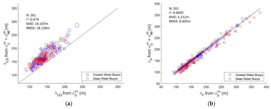
Figure 4.
Estimated azimuth cut-off wavelengths (a) and dominant wavelengths (b) from both VV and VH polarization NRCS data versus those from VV polarization NRCS data alone.
Generally, the cut-off wavelengths derived from the VV NRCS data are higher than those from the composite VV and VH NRCS data. Figure 4a shows the cut-off wavelengths from dual-polarization data (λco_VV+VH) versus those from the single-polarization data (λco_ VV). It is seen that for lower Hs, there is less difference between λco_ VV+VH and λco_ VV than for higher Hs.
Figure 5 shows the distribution of the estimated dominant wavelength and azimuth cut-off wavelength from the dual-polarization SAR spectra. The distribution of the dominant wavelength between different water depths is found to be similar, while in both areas, most of the wavelengths are around 100–175 m. The shortest wavelength that can be detected was approximately 100 m. In less than five SAR images of the deep-water regions, wavelengths below 100 m can be retrieved
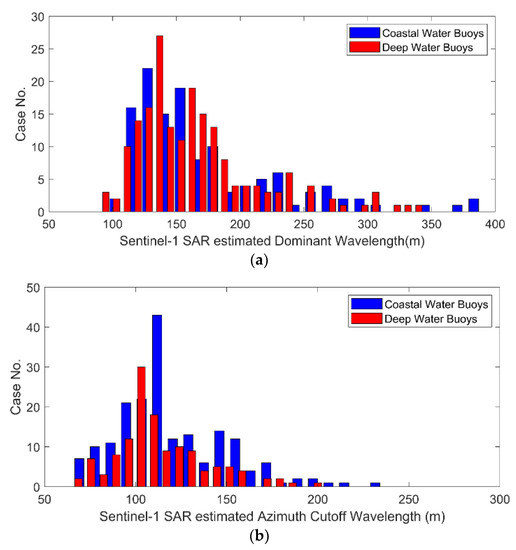
Figure 5.
Estimated dominant wavelength (a) and azimuth cut-off wavelength (b) distributions based on number of images.
4. Results and Analysis
Using the derived dominant wavelength (λp) and the cut-off wavelength (λco), the significant wave height (Hs) was calculated using Equations (15) and (16). The buoy data were used to validate the SAR data-derived Hs accuracy. Three statistical parameters were used to quantify the validation results, namely, the mean average error (MAE), the standard deviation of the error (SDE), the root mean square error (RMSE), and the coefficient of determination (r2) given by,
where N is the number of data, is in-situ measured parameter, yi is the estimated parameter, and .
The accuracy evaluation results of the derived Hs based on the SAR data are listed in Table 3. It shows that for all SAR images, the Hs estimation accuracy increased by using the dual-polarization strategy with the MAE, SDE, and RMSE as 0.41, 0.31, and 0.52 m, respectively versus those of 0.56, 0.44, and 0.69 m by using the single VV polarization data. The r2 value reaches 0.73 for the composite methodology versus 0.55 for the single polarization method, and for the MAE and RMSE, the Hs estimation relative error was reduced by ~10% and ~24% respectively. Table 3 reveals that relatively higher error values were found when U10 was lower than 4 ms−1, while lower errors were found in U10 higher than 4 ms−1. Figure 6 shows comparisons of the Hs estimation using both coastal (a, b) and deep-water SAR images (c, d) with the NDBC buoy measured Hs.
Table 3.
Comparison of results between SAR images and National Data Buoy Center (NDBC) buoy data.
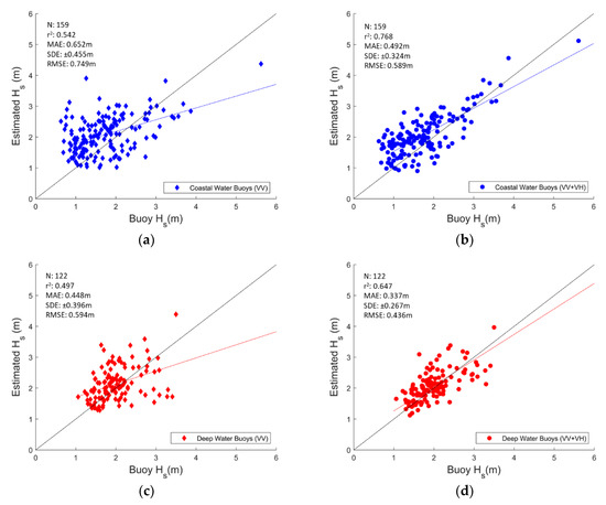
Figure 6.
Comparisons of the Hs estimation using both coastal (a,b) and deep water SAR images (c,d) using VV and VV + VH polarizations, respectively.
The dual-polarization strategy (b, d) exhibits better results than the single-polarization method both in the deep and coastal waters. As seen in Figure 6, the dual-polarization method, the Hs estimation accuracy increases for both low wind and high wind speeds and in both coastal and deep waters. Therefore, it is evident that the dual-polarization strategy can improve Hs estimation.
In addition, the deep-water dataset generally displayed better Hs estimation than that in the coastal water with higher r2 and lower MAE and RMSE. In general, the coastal SAR data resulted in higher errors of the Hs estimate when compared with the deep-water result, as shown by the MAE value. This is also supported by the comparison in the r2 value. In addition, the linear trend indicated an overestimation of the significant wave height in the coastal region for an Hs less than 2 m. Figure 7 shows the error distribution by comparing the SAR image-estimated Hs and data from NDBC buoys, and it also indicates that the estimation in coastal waters had larger errors than in deep water due to the overestimation.
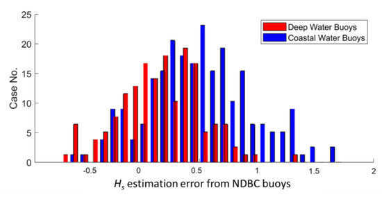
Figure 7.
Distribution of Hs estimation errors as compared with the NDBC buoy data for the coastal water and deep water.
5. Discussion
Our study shows that the lowest cut-off wavelength is approximately 90 m, similar to what was determined from previous studies [12,22]. The cut-off wavelength exists due to the complex velocity bunching of ocean waves and the high R/V ratio, resulting in the inability of a SAR sensor with multi-look capability to capture short waves in the azimuthal direction (velocity bunching). A system such as Real Aperture Radar, Airborne SAR or a satellite with a lower ratio of R/V would have a higher probability to image short ocean waves.
The significant wave heights derived from Sentinel-1 SAR images for 2017 in deep and coastal water are shown in Figure 8, together with buoy-measured Hs. Hs from the buoys of NDBC 51000 and NDBC 46054 co-located with the SAR images are also displayed to represent waves in the deep and coastal waters of the Pacific Ocean. The Pacific Ocean displays a wave climate of equatorial and near-equatorial storm systems. In addition, the tropics and subtropics have relatively mild easterly trade winds, with appreciable wave activities concentrated in the central North Pacific affecting both the Hawai’i region and the West Coast of the U.S. [51,52,53,54]. There were two to four SAR images per month at each buoy location, while the buoy observed Hs data are hourly. Figure 8 shows that both estimates of Hs are consistent with each other, except that the SAR data-derived Hs does not exhibit high frequency variability due to a lower temporal resolution. Long-term consistency between the SAR image-derived Hs products based on the new methodology and in-situ buoy observations both for the coastal and deep waters are consolidated in the comparison.
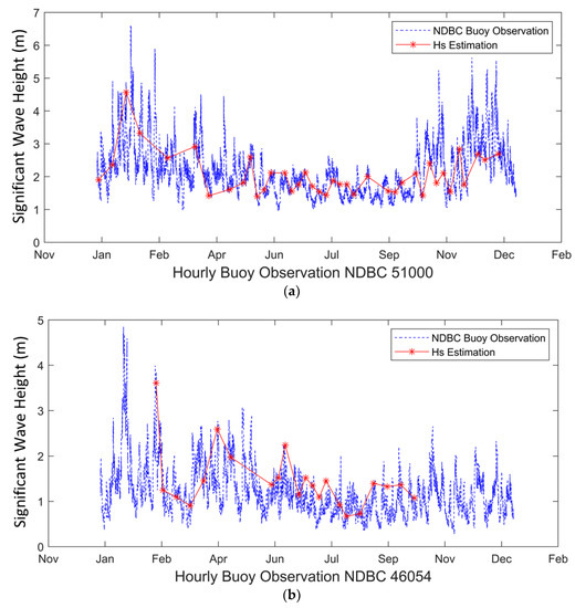
Figure 8.
Sentinel SAR data-derived Hs (in red), the NDBC buoy measured Hs (in blue) at stations 51000 (a) and 46054 (b) for 2017.
Previous investigations and this study demonstrated the capability of SAR sensors to observe ocean waves. For the remote sensing of ocean waves, satellite altimeters can also measure significant wave height with better sampling and accuracy along their ground tracks than the SARs. Altimeter Hs data have been available continuously since the early 1990’s with ~10% accuracy and widely used in global wave climate studies [55].
The altimeter Hs data have a spatial resolution of 2~10 km along satellite ground tracks, but in the cross-track direction, the Hs spatial resolution depends on the distance (about 100 km) between the neighbor ground tracks since the conventional altimeter does not image the ground surface. Compared with the satellite altimeter observations, the SAR imagery can provide Hs data with two important benefits over the altimeter, namely high spatial resolution in 2D directions concurrently with wave spectrum information, and retrieval of the wave information at high resolution close to coasts. Therefore, the SAR and altimeter Hs data can be used for different aspects, respectively. For ocean wave climate study on the basin scale, the altimeter can provide vast coverage of continuous Hs data, while SAR observations present wave fields with a high spatial resolution as fine as tens of meters, which is of great important to capture fine structures of wave fields especially in the coastal waters. It is believed that Hs observations from both satellite SARs and altimeters can enrich monitoring, prediction, and studies of ocean waves.
The results presented in Section 3 have demonstrated that there is a high probability of determining wavelength information from a two-dimensional wave spectrum. However, noise in SAR images may limit the accuracy of the retrieved dominant wavelength. The limitations of SAR images in detecting the ocean waves are due to noise-blurred surface wave streaks as well as by calm water surface in which the wave patterns are weak. Our results of significant wave height estimation show the applicability of a dual-polarization-enhanced methodology, which can be effective in both in coastal and deep waters, in both swell and wind wave dominant environment. Moreover, the utilization of a dual-polarization method can help to improve estimation accuracy of wave parameters under contrasting wind conditions, as shown in Table 2. However, several issues still need to be explored, such as the slight underestimation of deep-water Hs, and an improved understanding of the detailed physical processes of how the combination of co- and cross-polarizations of SAR images can filter out noises. Our future studies will incorporate more information by utilizing full-polarimetric SAR datasets in non-linear and multi-wave environments and conduct a detailed analysis of the Hs retrieval accuracy under different environmental conditions over a longer period.
6. Conclusions
In this study, an enhanced methodology using the dual-polarization (VV and VH) SAR images to estimate the significant wave height (Hs) was developed for deep and coastal water regions. Sentinel-1A and 1B SAR images at two test sites are employed to derive Hs from data taken from 2017. Hs measured from co-located NOAA buoys are also utilized to assess the results from satellite SAR data. For the two study sites, one is in the Hawai’i region for a deep-water scenario, and the other is around the Channel Islands on the West Coast of the USA for a coastal water scenario.
The study reveals that the utilization of dual-polarization SAR images enhances the estimate of the cut-off wavelength. For comparison, a VV polarization SAR image is also used to obtain the significant wave height. The validation results reveal that the MAE and RMSE of Hs is reduced by 26.7% and 24.6% respectively, with the SAR dual-polarization methodology as compared to that from the single-polarization SAR images, and r2 increases for the enhanced dual-polarization methodology in both deep and coastal waters. Long term comparison between satellite SAR derived Hs and the buoy data exhibits the robustness of the methodology.
In our study, the lowest possible estimated cut-off wavelength found was ~90 m, and the dominant wavelength is in the range of 105–175 m. This result suggests that waves with a wavelength shorter than 90 m might not be detectable for the SAR images in the azimuth direction. We reveal here that the composition of dual-polarization SAR images is better than a single polarization strategy, though the mechanism of the non-Bragg scattering that enhances the cut-off wavelength estimate and the role of non-Bragg scattering such as wave breaking in detecting the dominant waves in high sea states still need further explorations. Future studies will design new methodologies to correct the velocity bunching effects in order to discern short ocean surface waves and incorporate satellite altimetry systems such as Jason-3, Sentinel-3, and the upcoming Sentinel-6 missions, and wave data from operational hindcast models such as Wavewatch III and the Global Ocean Waves Analysis and Forecast datasets from the Copernicus Marine Environment Monitoring Service (CMEMS).
Author Contributions
Conceptualization, F.S.P. and J.P.; data curation, F.S.P.; formal analysis, J.P. and A.T.D.; funding acquisition, H.L.; methodology, F.S.P. and J.P.; software, F.S.P.; supervision, H.L.; validation, F.S.P. and J.P.; visualization, F.S.P.; writing—original draft, F.S.P. and J.P.; writing—review and editing, J.P., A.T.D. and H.L. All authors have read and agreed to the published version of the manuscript.
Funding
This study is jointly supported by the General Research Fund of Hong Kong Research Grants Council (RGC) under grants: CUHK 14303818, the National Natural Science Foundation of China under project 41376035, and the talent startup fund of Jiangxi Normal University.
Institutional Review Board Statement
Not applicable.
Informed Consent Statement
Not applicable.
Data Availability Statement
The Sentinel-1 SAR images are made publicly available by European Space Agency via https://scihub.copernicus.eu. Buoy data are available via http://www.ndbc.noaa.gov/. Figures are plotted using Matlab R2019b.
Acknowledgments
We would like to thank four anonymous reviewers for their valuable comments and suggestions that significantly help to improve the quality of the paper.
Conflicts of Interest
The authors declare no conflict of interest.
References
- Valenzuela, G.R. Theories for The Interaction of Electromagnetic and Oceanic Waves—A Review. Bound-Lay Meteorol. 1978, 13, 61–85. [Google Scholar] [CrossRef]
- Alpers, W.; Ross, D.D.; Rufenach, C.L. On the detectability of ocean surface waves by real and synthetic aperture radar. J. Geophys. Res. 1981, 86, 6481–6498. [Google Scholar] [CrossRef]
- Alpers, W. Theory of radar imaging of internal waves. Nature 1985, 314, 245–247. [Google Scholar] [CrossRef]
- Yang, C.-S.; Ouchi, K. Application of Velocity Bunching Model to Estimate Wave Height of Ocean Waves using Multiple Synthetic Aperture Radar Data. J Coast. Res. 2017, 79, 94–98. [Google Scholar] [CrossRef]
- Marghany, M.; Ibrahim, Z.; van Genderen, J.L. Azimuth Cut—Off Model for Significant Wave Height Investigation along Coastal Water of Kuala Terengganu, Malaysia. Int. J. Appl. Earth. Obs. Geoinf. 2002, 4, 147–160. [Google Scholar] [CrossRef]
- Susanto, R.D.; Mitnik, L.; Zheng, Q. Ocean internal waves observed in the Lombok Strait. Oceanography 2005, 18, 80–87. [Google Scholar] [CrossRef]
- Hersbach, H.; Stoffelen, A.; de Haan, S. An improved C-band scatterometer ocean geophysical model function: CMOD5. J. Geophys. Res. 2007, 112, 225–237. [Google Scholar] [CrossRef]
- Shao, W.Z.; Zhang, Z.; Li, X.; Li, H. Ocean Wave Parameters Retrieval from Sentinel-1 SAR Imagery. Remote Sens. 2016, 8, 707. [Google Scholar] [CrossRef]
- Bioresita, F.; Puissant, A.; Stumpf, A.; Malet, J.P. A Method for automatic and Rapid Mapping of Water Surfaces from Sentinel-1 Imagery. Remote Sens. 2018, 10, 217. [Google Scholar] [CrossRef]
- Plank, S. Rapid Damage Assessment by Means of Multi-Temporal SAR—A Comprehensive Review and Outlook to Sentinel-1. Remote Sens. 2014, 6, 4870–4906. [Google Scholar] [CrossRef]
- Chapron, B.; Johnsen, H.; Garello, R. Wave and wind retrieval from sar images of the ocean. Ann. Télécommun. 2001, 56, 682–699. [Google Scholar]
- Pramudya, F.S.; Pan, J.; Devlin, A.T. Estimation of Significant Wave Height of Near-Range Traveling Ocean Waves Using Sentinel-1 SAR Images. IEEE J. Sel. Top. Appl. Earth. Obs. Remote. Sens. 2019, 12, 1067–1075. [Google Scholar] [CrossRef]
- Hasselmann, K.; Hasselmann, S. On The Nonlinear Mapping of an Ocean Wave Spectrum Into a Synthetic Aperture Radar Image Spectrum. J. Geophys. Res. 1991, 96, 10713–10729. [Google Scholar] [CrossRef]
- Hasselmann, S.; Bruning, C.; Hasselmann, K. An improved algorithm for the retrieval of ocean wave spectra from synthetic aperture radar image spectra. J. Geophys. Res. Oceans 1996, 101, 16615–16629. [Google Scholar] [CrossRef]
- WAMDI Group. The WAM Model—A third-generation ocean wave prediction model. J. Phys. Oceanogr. 1988, 18, 1775–1810. [Google Scholar] [CrossRef]
- Mastenbroek, C.; De Valk, C.F. A semiparametric algorithm to retrieve ocean wave spectra from synthetic aperture radar. J. Geophys. Res. Oceans 2000, 105, 3497–3516. [Google Scholar] [CrossRef]
- Sun, J.; Guan, C.L. Parameterized first-guess spectrum method for retrieving directional spectrum of swell-dominated waves and huge waves from SAR images. Chin. J. Oceanol. Limn. 2006, 24, 12–20. [Google Scholar]
- Lin, R.; Yang, J.; Mouche, A. Preliminary analysis of Chinese GF-3 SAR Quad-polarization measurements to extract winds in each polarization. Remote Sens. 2017, 9, 1215. [Google Scholar]
- Schulz-Stellenfleth, J.; Konig, T.; Lehner, S. An empirical approach for the retrieval of integral ocean wave parameters from synthetic aperture radar data. J. Geophys. Res. 2007, 112, 1–14. [Google Scholar] [CrossRef]
- Li, X.M.; Lehner, S.; Bruns, T. Ocean wave integral parameter measurements using Envisat ASAR wave mode data. IEEE Trans. Geosci. Remote Sens. 2011, 49, 155–174. [Google Scholar] [CrossRef]
- Stopa, J.E.; Mouche, A. Significant wave heights from Sentinel-1: Validation and applications. J. Geophys. Res. Oceans 2017, 122, 1827–1848. [Google Scholar] [CrossRef]
- Kerbaol, V.; Chapron, B.; Vachon, P.W. Analysis of ERS-1/2 Synthetic Aperture Radar Wave Mode Imagettes. J. Geophys. Res. 1998, 115, 7833–7846. [Google Scholar] [CrossRef]
- Stopa, J.E.; Ardhuin, F.; Chapron, B. Estimating wave orbital velocity through the azimuth cut-off from spaceborne satellites. J. Geophys. Res. Oceans. 2015, 120, 7616–7634. [Google Scholar] [CrossRef]
- Wang, H.; Zhu, J.; Yang, J.; Shi, C. A semi-empirical algorithm for SAR wave height retrieval and its validation using Envisat ASAR wave mode data. Acta Oceanol. Sin. 2012, 31, 59–66. [Google Scholar]
- Hua, F.; Fan, B.; Lu, Y.; Wang, J. An empirical relation between sea wave spectrum peak period and zero-crossing period. Adv. Mar. Sci. 2004, 22, 16–22. [Google Scholar]
- Sun, J.; Kawamura, H. Surface wave parameters retrieval in coastal seas from spaceborne SAR image mode data. Prog. Electromagn. Res. 2008, 4, 445–450. [Google Scholar] [CrossRef][Green Version]
- Ren, L.; Yang, J.S.; Zheng, G.; Wang, J. Significant wave height estimation using azimuth cut-off of C-band RADARSAT-2 single-polarization SAR images. Acta Oceanol. Sin. 2015, 12, 1–9. [Google Scholar] [CrossRef]
- Grieco, G.; Nirchio, F.; Migliaccio, M.; Portabella, M. Dependency of The Sentinel-1 Azimuth Wavelength Cut-Off on Significant Wave Height and Wind Speed. Int. J. Remote Sens. 2016, 37, 5086–5104. [Google Scholar] [CrossRef]
- Li, J.; Holt, M. Comparison of Envisat ASAR Ocean Wave Spectra with Buoy and Altimeter Data via a Wave Model. J. Atmos. Oceanic Technol. 2009, 26, 593–614. [Google Scholar] [CrossRef]
- Sheng, Y.; Shao, W.; Zhu, S.; Jian, S.; Xinzhe, Y.; Shuiqing, L.; Jian, S.; Juncheng, Z. Significant Wave Height Retrieval from Co-Polarization Chinese Gaofen-3 SAR Imagery Using an Improved Algorithm. Acta Oceanol. Sin. 2018, 37, 1–10. [Google Scholar] [CrossRef]
- Shao, W.Z.; Sheng, Y.X.; Sun, J. Preliminary assessment of wind and wave retrieval from Chinese Gaofen-3 SAR imagery. Sensors 2017, 17, 1705. [Google Scholar] [CrossRef] [PubMed]
- Yang, J.S.; Ren, L.; Wang, J. The first quantitative remote sensing of ocean surface waves by Chinese GF-3 SAR satellite. Oceanol. Limnol. Sin. 2017, 48, 207–209. [Google Scholar]
- European Space Agency. Sentinel-1 Acquisition Modes. Available online: https://sentinel.esa.int/web/sentinel/technical-guides/sentinel-1-sar/sar-instrument/acquisition-modes (accessed on 9 October 2020).
- Valenzuela, G.R. Depolarization of E.M. Waves by Slightly Rough Surfaces. IEEE Trans. Antennas Propag. 1967, AP-15, 552–557. [Google Scholar] [CrossRef]
- Hauser, D.; Kahma, K.K.; Krogstad, H.E. Measuring and Analyzing the Directional Spectra of Ocean Waves; E.U. Publications Office: Luxembourg, 2003; pp. 15–54. [Google Scholar]
- Lee, J.S.; Wen, J.H.; Ainsworth, T. Improved sigma filter for speckle filtering of SAR imagery. IEEE Trans. Geosci. Remote Sens. 2009, 47, 202–213. [Google Scholar]
- Mouche, A.; Chapron, B. Global C-Band Envisat, RADARSAT-2 and Sentinel-1 SAR Measurements in Copolarization and Cross-Polarization. J. Geophys. Res. 2015, 120, 7195. [Google Scholar] [CrossRef]
- Kudryavtsev, V.N.; Chapron, B.; Myasoedov, A.G.; Collard, F.; Johannessen, J.A. On Dual Co-Polarized SAR Measurements of the Ocean Surface. IEEE Geosci. Remote Sens. Lett. 2013, 10, 761–765. [Google Scholar] [CrossRef]
- Kudryavtsev, V.N.; Fan, S.; Zhang, B.; Mouche, A.A.; Chapron, B. On Quad-Polarized SAR Measurements of the Ocean Surface. IEEE Trans. Geosci. Remote Sens. 2019, 57, 8362–8370. [Google Scholar] [CrossRef]
- Zhang, B.; Perrie, W.; Vachon, P.W.; Li, X.; Pichel, W.G.; Guo, J.; He, Y. Ocean vector winds retrieval from C-band fully polarimetric SAR measurements. IEEE Trans. Geosci. Remote Sens. 2012, 50, 4252–4261. [Google Scholar] [CrossRef]
- Voronovich, A.; Zavorotny, V. Full-polarization modeling of monostatic and bistatic radar scattering from a rough sea surface. IEEE Trans. Antennas Propag. 2014, 62, 1362–1371. [Google Scholar] [CrossRef]
- Zhang, B.; Perrie, W. Recent progress on high wind-speed retrieval from multi-polarization SAR imagery: A review. Int. J. Remote Sens. 2014, 35, 4031–4045. [Google Scholar] [CrossRef]
- Xie, T.; Perrie, W.; Zhang, G.; Yang, J.; He, Y. Comparison of C-Band Quad-Polarization Synthetic Aperture Radar Wind Retrieval Models. Remote Sens. 2018, 10, 1448. [Google Scholar]
- Fois, F.; Hoogeboom, P.; Le Chevalier, F.; Stoffelen, A. Future ocean scatterometry: On the use of cross-polar scattering to observe very high winds. IEEE Trans. Geosci. Remote Sens. 2001, 39, 2601–2612. [Google Scholar] [CrossRef]
- Corcione, V.; Nunziata, F.; Migliaccio, M. Megi Typhoon Monitoring by X-Band Synthetic Aperture Radar Measurements. IEEE J. Ocean. Eng. 2018, 43, 184–194. [Google Scholar] [CrossRef]
- Zhang, G.; Li, X.; Perrie, W.; Hwang, P.A.; Zhang, B.; Yang, X. A Hurricane Wind Speed Retrieval Model for C-Band RADARSAT-2 Cross-Polarization ScanSAR Images. IEEE Trans. Geosci. Remote Sens. 2017, 55, 4766–4774. [Google Scholar] [CrossRef]
- Corcione, V.; Grieco, G.; Nunziata, F.; Migliaccio, M. A New Azimuth Cut-Off Procedure to Retrieve Significant Wave Height Under High Wind Regimes. In Proceedings of the IEEE International Geoscience and Remote Sensing Symposium (IGARSS 2018), Valencia, Spain, 22–27 July 2018; pp. 6057–6059. [Google Scholar]
- Nunziata, F.; Gambardella, A.; Migliaccio, M. An educational SAR sea surface waves simulator. Int. J. Remote Sens. 2008, 29, 3051–3066. [Google Scholar] [CrossRef]
- Beal, R.C.; Tilley, D.G.; Monaldo, F.M. Large and Small Scale Spatial Evolution of Digitally Processed Ocean Wave Spectra from Seasat Synthetic Aperture Radar. J. Geophys. Res. 1983, 88, 1761–1778. [Google Scholar] [CrossRef]
- Goldfinger, A.D. Estimation of Spectra from Speckled Images. IEEE Trans. Aerosp. Electron. Syst. 1982, AES-18, 675–681. [Google Scholar] [CrossRef]
- Hemer, M.; Church, J.; Hunter, J. Variability and trends in the directional wave climate of the Southern Hemisphere. Int. J. Climatol. 2009, 30, 475–491. [Google Scholar] [CrossRef]
- Arinaga, R.A.; Cheung, K.F. Atlas of global wave energy from 10 years of reanalysis and hindcast data. Renew. Energy 2012, 39, 49–64. [Google Scholar] [CrossRef]
- Bromirski, P.D.; Cayan, D.R.; Flick, R.E. Wave spectral energy variability in the northeast Pacific. J. Geophys. Res. Space Phys. 2005, 110, 110. [Google Scholar] [CrossRef]
- Ribal, A.; Young, I.R. 33 years of globally calibrated wave height and wind speed data based on altimeter observations. Sci. Data 2019, 6, 77. [Google Scholar] [CrossRef] [PubMed]
- Young, I.R.; Donelan, M.A. On the determination of global ocean wind and wave climate from satellite observations. Remote Sens. Environ. 2018, 215, 228–241. [Google Scholar] [CrossRef]


Publisher’s Note: MDPI stays neutral with regard to jurisdictional claims in published maps and institutional affiliations. |
© 2021 by the authors. Licensee MDPI, Basel, Switzerland. This article is an open access article distributed under the terms and conditions of the Creative Commons Attribution (CC BY) license (http://creativecommons.org/licenses/by/4.0/).