Abstract
Identifying the rapeseed (Brassica napus L.) flowering dates are important for planting area estimation, growth monitoring, and yield estimation. However, there is currently a lack of data on rapeseed flowering dates at the parcel scale. In this study, a new spectral index (Normalized Rapeseed Flowering Index, NRFI) is proposed to detect rapeseed flowering dates from time series data generated from Landsat 8 OLI and Sentinel-2 sensors. This study also analyzed the feasibility of using the backscattering coefficients (VV, VH, and VV/VH) of Sentinel-1 to detect the flowering dates of rapeseed at the parcel scale. Based on the spectral and polarization characteristics of 718 rapeseed parcels collected in 2018, we developed a method to automatically identify peak flowering dates by the local maximum of NRFI series and the local minimum of VH and VV, along with the maximum of VV/VH. The results show that most of the peak flowering dates derived from Sentinel-1 and Sentinel-2 can be confirmed by the in-situ phenological observations at the Deutscher Wetterdienst (DWD) stations in Germany. The NRFI outperforms the Normalized Difference Yellow Index (NDYI) in identifying the peak flowering dates from Landsat 8. The derived medians of peak flowering dates by NRFI, NDYI (Sentinel-2), and VH are similar, while a systematic delay is observed by NDYI (Landsat 8). The method with the spectrum and backscattering coefficients will be a potential tool to identify crop flowering dynamics and map crop planting area.
1. Introduction
Rapeseed (Brassica napus L.) is a staple oil crop used for cooking, high-quality animal feed, etc. [1]. It is cultivated widely in the world (e.g., Europe, Canada, China, India, and Australia) [2,3,4,5]. The global rapeseed production has grown rapidly in recent years [6]. The timing and intensity of flowering are closely related to the final yield of rapeseed [2,7,8,9] and highly sensitive to temperature [2,10], as other crops [11,12,13]. For instance, sclerotinia stem rot can cause a 50% yield loss when the rapeseed is in bloom [14]. Additionally, the accurate flowering dates are key information to map rapeseed planting areas [15,16]. The peak flowering period is highly informative for monitoring growth status and predicting yield [2,17]. Therefore, it is of vital importance to accurately identify the flowering dates of rapeseed. Given the high spatial heterogeneities of cultivars, farmers’ management practices, climate, and soil conditions, it is still challenging to detect the peak flowering dates of rapeseed timely and soundly [18].
Remote sensing data (e.g., optical and radar images) have become a powerful tool to derive biophysical parameters including crop phenological information in the last decades [18,19,20,21,22,23]. Among other things, optical data have prevailed to analyze the relationship between the photosynthetic and properties of crops, mostly via the conventional Normalized Difference Vegetation Index (NDVI) and the Enhanced Vegetation Index (EVI) when an unprecedented amount of free satellite data become available [24,25]. The previous works have proved that rapeseed flowering dates can be detected by optical remote sensing [5]. For example, Sulik et al. [18] showed spectral information on optical data may improve rapeseed flowering identification. Later, a new index called the Normalized Difference Yellowness Index (NDYI) was proposed, whose performance was better than NDVI for monitoring the peak flowering period of rapeseed [17]. Using NDYI from Sentinel-2, Andrimont et al. [2] had successfully detected rapeseed peak flowering dates in Germany. Sentinel-2 is an earth observation mission from the Copernicus Programme [22], which is being operated by the European Space Agency (ESA). Sentinel-2 was first launched in 2015 (https://sentinel.esa.int/web/sentinel/home) so no Sentinel-2 images are available for monitoring the flowering phenology of rapeseed before 2015. The Landsat was first launched in 1972 and is the longest-running enterprise to better understand global environmental change and agricultural practices (https://www.nasa.gov/mission_pages/landsat/overview/index.html). Landsat 8 was launched in 2013 [23]. Therefore, compared with Sentinel-2, Landsat is a better source for monitoring historical agricultural practices, although Landsat has a lower capability (e.g., lower ground resolution). However, the applicability of the existing Sentinel-2 based method for detecting rapeseed flowering phenology to Landsat still needs to be explored.
The traditional approaches based on the optical data show some limitations to detecting the flowering dates of rapeseed during cloudy days [14,26,27]. Compared with optical remote sensing, synthetic aperture radar (SAR) data is not affected by clouds. The time trajectory of many crops from SAR can be explained with various frequencies and incidence angles based on electromagnetic modeling [10,16,28,29]. Recently, many studies have proved that the backscatter coefficients (VV, VH, and VV/VH) of various crops would change with their phenological development, suggesting that the changes of backscatters with phenology should be mainly driven by the structural changes during crop growth [14,16,21,30,31,32,33]. Given the different structures of crop canopies, it would be easily concluded that rapeseed in the field can be detected by the three backscatters of C-band sensors [2,32,34]. Many studies have found several radar features will change as rapeseed grows [2,14,15,16,31,32]. Moreover, the previous study has substantiated that the scattering coefficient VV can detect the peak flowering of rapeseed [2].
However, our understanding of the spatiotemporal dynamics of rapeseed flowering dates has been very limited so far due to very few observation data available. Most of the existing yellowness indices (e.g., NDYI) require hyperspectral data or an unmanned aerial vehicle [35,36,37], which constrain their wide application. Thus, a novel and widely accepted method to detect rapeseed flowering dynamics is highly required. Understanding the effects of specific flowering stages on the structural and spectral properties of rapeseed flowering may provide ideas for developing effective methods to detect rapeseed flowering dynamics [2,38].
Thus, the objectives of this study are: (a) explore the reflectance values of rapeseed during the growing period and develop a new index (Normalized Rapeseed Flowering Index, later called as NRFI) to monitor the peak flowering dates, then compare its performance with the NDYI; (b) demonstrate the ability of backscatter (VV, VH, VV/VH) to characterize the critical rapeseed peak flowering parameters; (c) compare the consistency of the detected peak flowering dates based on the spectral indexes and radar together with the developed methods.
2. Materials and Methods
2.1. DWD Station and Study Area
Germany is a major rapeseed growing region in Europe. Germany’s national meteorological service (DWD) maintains a database of phenological observations [39]. The dataset has been used in many previous studies, especially for advice for agriculture [39]. The dataset contains field records of crop phenological stages following the BBCH (Biologische Bundesantalt, Bundessortenamt, and Chemische Industrie) scale [40]. For rapeseed, the start (i.e., BBCH61) and end (i.e., BBCH69) of flowering dates are available, while the peak flowering dates (i.e., BBCH65) are not. Each record associated with a DWD station is considered to represent a crop within a maximum distance of five kilometers from its location [2,40]. A total of 268 rapeseed observation sites with complete records were obtained from the DWD phenology database in 2018. We analyzed the flowering start dates, end dates, and flowering period recorded at all these stations (Figure 1). The flowering of rapeseed starts usually around the 110th day and ends mainly around the 135th day of the year in Germany. The flowering period lasts for mostly 20~30 days—a considerable portion of the growing season [18]. Among these observation stations, 22 stations were selected for further analyses (Figure 2a) because five L8 images and five S2 images were available from April to June, which covered all these 22 stations.
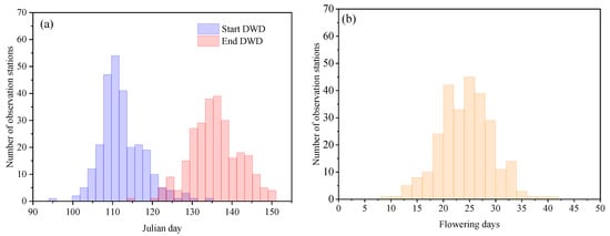
Figure 1.
The start and end dates of flowering (a) and length of the flowering periods (flowering days) (b), for rapeseed based on Germany’s national meteorological service (the Deutscher Wetterdienst, DWD) observations. The y-axis represents the number of observation stations. The x-axis of (a,b) represent Julian day and flowering days, respectively.
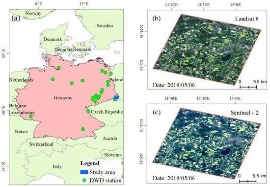
Figure 2.
Germany’s National Meteorological Service (the Deutscher Wetterdienst, DWD) stations of rapeseed (a), Landsat 8 (b), and Sentinel-2 (c) images during the flowering period of rapeseed. The true color composites (R/G/B = Band4/Band3/Band2) from Landsat 8 OLI and Sentinel-2 images.
2.2. Identifying the Rapeseed Parcels
Compared with other land-use types, rapeseed has unique spectral characteristics during the flowering period. It appears green-yellow or yellow in the image of a combination of red, green, and blue bands. Thus, the visual interpretation of rapeseed parcels is based on the specific spectral feature [3,32,35,41,42]. Rapeseed flowering dates vary by location due to differences in climate, cultivars, and agricultural management [2] (Figure 1). We extracted 718 parcels from a region (51°17′00″–50°56′43″ N, 14°34′13″ N–15°8′10″ E) where the image quality of Sentinel-1/2 was good during the rapeseed growing season, and rapeseed was widely cultivated as a winter crop (Figure 2b,c). The visual interpretation was based on high-resolution Google earth images and Sentinel-2 images.
2.3. Satellite Data
2.3.1. Optical Satellite
All the available optical satellite data from Landsat 8 OLI and Sentinel-2 sensors at the Google Earth Engine (GEE) platform in 2018 were used in this study. The spatial resolutions of L8 true-color images and S2 images were 30 and 10 m, respectively. The S2 top-of-atmosphere reflectance archived in the GEE was processed by radiometric and geometric corrections including orthorectification and spatial registration on a global reference system with sub-pixel accuracy [43,44,45]. The GEE asset addresses of L8 and S2 are LANDSAT/LT08/C01/T1_SR and COPNERICUS/S2, respectively. We used a cloud-score algorithm to remove the clouds, cloud shadows, and snow/ice pixels [2,46].
2.3.2. SAR Satellite
We collected the Sentinel-1A/B C-band Synthetic Aperture Radar (SAR) data. Sentinel-1A/B provides a series of SAR images. The period of S1 data ranges from 2 to 12 days due to the differences in data types and regions all around the world [47]. For a denser time series, the ascending and descending orbit observations were combined [2,47]. The temporal resolution of S1 data in 2018 was two days, with a high spatial resolution (10× 10 m). The interferometric Wide Swath (IW) instrument mode with VV and VH was also used in the study [47]. The multi-temporal speckle filter at the GEE platform was applied to remove the noise of the backscatter S1 images [48]. Finally, we analyzed the temporal backscatter values of VV, VH, and VV/VH polarization over the rapeseed field during different phenological stages of rapeseed.
2.4. Developing a New Index—NRFI to Catch Flowering Dynamics
Reflectance values of green and red bands change considerably during flowering stages of rapeseed according to previous studies [18,38]. The large changes in the two bands are useful to catch their dynamics. We believe the green/red bands from L8 and S2 provide valuable information to develop the NRFI. Most previous studies on rapeseed phenology substantiated the values of visible light bands [2,3,10,14,15,17,18,34,38,42,49], very few have focused on the rapeseed phenology characteristics of the short-wave infrared band (SWIR). The SWIR is less influenced by the atmosphere and more sensitive to water content in soil or plant [50]. Considering the potential different responses between green/red and SWIR2 bands to the flowering processes of rapeseed, this paper constructed a novel index to capture the flowering intensity of rapeseed—Normalized Difference Rapeseed Flower Index (NRFIr/NRFIg)—see Equations (1) and (2). The NRFIr and NRFIg are based on one visible band (green/red) and one invisible band (SWIR2).
where , , , are blue (B2: 450–520/515 nm), green (B3: 520–600 nm), red (B4: 630–690/680 nm), and short-wave infrared 2 (B7: 2100–2300 nm) bands of Landsat 8 OLI/ Sentinel-2 MSI imagery, respectively. NRFI is defined either for red bland-specific (NRFIr) or green band-specific (NRFIg), which is determined after comparing their performances in identifying the flowering period of rapeseed.
2.5. Detecting Peak Flowering Stages
The peak flowering dates of rapeseed were identified based on a time series of remote sensing data. This study developed an approach to calculate the extrema of NRFI (Normalized Difference Rapeseed Flowering Index), NDYI, and backscatter values. Different smoothing methods could lead to large uncertainty in the retrieval of phenology [2,51]. The Savitzky-Golay (S-G) filter were used to smooth the time series of VV, VH, and VV/VH for each rapeseed parcel [52,53]. However, we didn’t apply the S-G filter to smooth L8 and S2 time series due to their coarser temporal resolutions, and the filtering algorithm could ignore local features and cause large uncertainties [52,53]. The peak flowering period was then obtained through the local maximum of NDYI, NRFI, and VV/VH along with the local minimum of VV and VH for all parcels during the expected flowering period (from 21 April to 30 May). The window size of the S-G filter was three and it was implemented using the TIMESAT 3.1 software. For the specific implementation process, please refer to reference [54].
2.6. Evaluating the Peak Flowering Stages Derived from the New Method
Although the starts and ends of the flowering stage were recorded in the DWD observations, the peak flowering stages were not [39]. We verified the detected peak flowering dates and the accuracy through two steps (Figure 3). First, we tested whether the flowering peak dates identified by our proposed method were between the start dates and the end dates recorded by the DWD stations. Second, the peak flowering dates identified by the two NRFIs from L8 and S2, and VH and VV/VH from S1 were compared with those detected by the two NDYIs from L8 and S2, and VV from S1. The previous study proved the accuracy of S2 NDYI and S1 VV by identifying the peak flowering of rapeseed based on a large amount of field survey data [2]. We used the Pearson correlation coefficient (r) (Equation (4)) and symmetric index of agreement (λ) (Equation (5)) to quantitatively assess the consistency of the peak flowering dates computed by L8, S1, and S2 time series [55,56].
where and denote the mean values of X and Y, respectively. and represent the standard deviations of X and Y, respectively. The metric r is dimensionless, with a range from −1 to 1. A value of zero indicates there is no linear dependence between the two variables, while a value close to 1 indicates significantly positive.
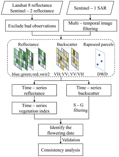
Figure 3.
Workflow of monitoring rapeseed flowering phenology in this study. Major modules include (1) data (Landsat 8 and Sentinel-1/2) preprocessing, (2) the extractions of time series of rapeseed reflectance, vegetation index (VI) and backscatter coefficients, (3) rapeseed flowering monitoring, (4) validation based on the field observation from DWD stations, and (5) the consistency analysis of rapeseed flowering phenology monitored by different indicators.
The advantage of the symmetric index of the agreement is that the index indicates how similar the values of the series are in magnitude [38,56].
3. Results
3.1. Spectral Properties and NDVI Phenological Characteristics of Rapeseed
Three different canopy morphologies are in the sequence indicated with the development of rapeseed, which is characterized by leaves, yellow flowers, and pods, respectively [35]. Rapeseed will appear yellowish-green on the image when it begins flowering. The color becomes yellow when rapeseed is approaching peak flowering (Figure 4a–e). Corresponding to the true color images above, the time series of spectral reflectance is shown in Figure 4f,g, which represents the mean values of 718 rapeseed parcels in four bands including blue, green, red, and SWIR2. The red and green bands increase as rapeseed begins flowering, peak at the medium flowering dates, and then decrease until the end of flowering for both L8 (Figure 4f) and S2 (Figure 4g). Moreover, their green bands display the highest reflectance, and the blue bands the lowest, with the red and SWIR2 bands in the middle, during the flowering period (Figure 4f,g). Reflectance values of the green and red bands in S2 changed from 0.11 and 0.079 (on Julian day 99) to 0.154 and 0.13 (on Julian day 109), respectively. While reflectance values of the green and red bands in L8 changed from 0.0695 and 0.05031 (on Julian day 99) to 0.1338 and 0.1177 (on Julian day 109), respectively. Previous research indicates that yellow flowers could increase red reflectance [57]. For rapeseed, the most distinguishable spectral difference between flowering and non-flowering can be identified by the green and red bands, which is consistent with previous studies [2,18,35,38,49,57]. The yellow rapeseed petals (e.g., carotene) increase the reflectivity of the red and green bands [17,18]. Thus, the red and green bands of rapeseed reach a local maximum during the peak flowering period (Figure 4f,g).
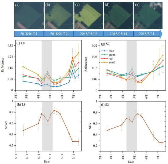
Figure 4.
True color images of Sentinel-2 with their dates shot (a–e) in 2018 and (f) time series of the blue, green, red, and SWIR2 bands of L8; (g) the time series of the blue, green, red and SWIR2 bands of S2; (h) the time series of L8 the normalized difference vegetation index (NDVI); (i) S2 NDVI. The gray area indicates the flowering dates recorded by the DWD stations. Means are indicated by dots and standard deviations by error bars.
Comparing with the “inverse V” curves of green and red values from L8 and S2 (Figure 4f,g), their NDVI values show a completely different “V” shape (Figure 4h,i). The NDVI values are high at the start and end of the flowering period, but low at the peak flowering stage, and reach the minimum at ripening [10]. NDVI values of L8 and S2 reduce from 0.78 and 0.66 to about 0.64 and 0.59 at the peak flowering stage, respectively, and then increase to the maximums (0.83 and 0.75) at the end of flowering. During the ripening stage, both NDVI decline to around 0.25. The NDVI dynamics are consistent with many previous studies [2,3,5,38,49]. For example, Pan et al. [35] indicated a decrease in NDVI values during the flowering period (BBCH65) up to 0.35, which was caused by the increase in red reflectance. For other crops such as wheat and corn, NDVI values do not change significantly during the flowering period [14]. Therefore, the unique spectral characteristics of rapeseed during the flowering period would provide a strong signal to identify and monitor the rapeseed flowering stage [5,14,38].
3.2. NRFI Better Characterize the Flowering Intensity
At peak flowering stages, the reflectance values of the green and red bands have a considerable increase, however, the values of SWIR2 are lower than those of the two visible bands (Figure 4f,g), which can provide valuable information to identify the rapeseed flowering period. The time series of spectral indices are extracted and averaged for the 718 rapeseed parcels (Figure 5). The flowering intensity signals are captured well by NRFIr from L8 (Figure 5a) and S2 (Figure 5b), with NRFIr showing a typical “reverse V” shape during the flowering period. Moreover, such a “reverse V” signature is also characterized by NDYI of S2, with NDYI showing a peak between the start and end of flowering stages recorded at DWD stations. However, two similar flattened peaks of NDYI and NRFIg from L8 (Figure 5a) and one lagged peak of NRFIg (Figure 5b) were also observed, which suggests the peak signals for flowering identified by the indexes have fallen beyond their actual flowering stages. Nevertheless, all values beyond the flowering stages were consistently lower than those within flowering stages during the whole growing period of rapeseed. Moreover, compared with the other two indexes, NRFIr performed best to capture the real signal of flowering dynamics from L8. The good performance of NRFIr is consistent with NDYI from S2, substantiated by several previous studies focused on field survey data [2,17]. The different curves of the indexes between L8 and S2 may ascribe to their different wavelengths [58,59]. Based on the comprehensive analysis of 718 rapeseed parcels, NRFIr is a reliable indicator to monitor the flowering intensity of rapeseed. Therefore, we will focus on NRFIr in the analyses hereafter, and all NRFI hereafter means NRFIr.
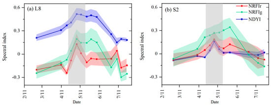
Figure 5.
The time series of normalized difference yellow index (NDYI), NRFIr, and NRFIg at the 718 rapeseed parcels. (a) for L8; (b) for S2. The gray area indicates the flowering dates recorded by the DWD. Dots indicate the mean values, and the filled color areas indicate the standard deviations across the 718 parcels.
3.3. Radar Polarization Characteristics of Rapeseed
The canopy structure changed dramatically as the rapeseed developed buds, flowers, and formed pods [32,35]. The backscatter and randomness in scattering changed with the processes of plant growth and was indicated morphologically by the change in canopy structure [32]. Thus, the time series of VV, VH, and VV/VH will inform us more on rapeseed growth states (Figure 6). VV backscatter values decrease sharply from the start of flowering, then reach a minimum in the middle of flowering, and increase sharply again till the end of flowering (Figure 6a). VH behaved similarly with VV but more gently, which was indicated by a more flat “V” curve (Figure 6b). This finding is supported by Wiseman et al. [60] based on RADARSAT-2 data [60]. As for S1, the backscatter values of the VV and VH changed from 0.11 and 0.079 (on Julian day 99) to 0.154 and 0.13 (on Julian day 109), respectively. Our findings are consistent with in-situ observations conducted by d’Andrimont et al. [2], which showed that the VV of S1 reached a local minimum during the peak flowering period of rapeseed. Moreover, the specific canopy structure of rapeseed might also contribute to the “V” shape during the flowering period. 1) The leaves and pods from neighboring plants are often intertwined to form a dense, randomly oriented canopy structure [14,15,31,32]. 2) As a strong back-scatter signal, stems, and pods of rapeseed, especially leaves, have characteristic sizes that are in the same order as the incident microwave wavelength [2,15]. 3) The smaller structured buds and flowers create a temporary layer of less effective scatters, which partly impedes the scattering of the underlying canopy, resulting in a decrease in VV scattering [2,14,60,61].
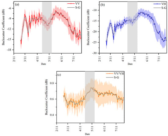
Figure 6.
The time series of VV (a), VH (b), and VV/VH (c). The gray area indicates the flowering dates recorded by the DWD. Dots indicate the means and the color-filled area indicates the standard deviations across the 718 parcels.
Furthermore, VV/VH increases as rapeseed enter the flowering stage and reach the maximum at the full flowering stage (Figure 6c). Considering their different responses during the stage (a sharp “V” in Figure 6a vs. a flat “V” in Figure 6b), rapeseed is randomly organized without a strong vertical structure during the flowering period. Furthermore, another advantage of selecting the ratio VV/VH as an index is that it can reduce the double-bounce effect and probably reduce errors from the acquisition system (e.g., due to the radiometric stability) or environmental factors (e.g., due to variations of soil moisture) [14]. Additionally, the VV/VH of the flowering period is the maximum during the whole growth period, while VH and VV are the local minimums. Therefore, VV/VH might be a more suitable indicator than VH or VV backscatter for monitoring the flowering period of rapeseed.
3.4. Comparing the Different Indexes for Monitoring Peak Flowering
To determine whether the peak flowering dates identified from satellites are within the ranges from the start to end of flowering observed at DWD stations, we further summarized the results in Figure 7 for comparisons. The flowering peak dates obtained from NRFIr, VV, VH, and NDYI (S2) fall within the ranges, but 59% of them from NDYI (L8) are beyond the range (Figure 7). Also, the spatial distribution of the peak flowering dates of rapeseed pixels based on NDYI (L8) and NRFIr (L8) shows that NRFIr (L8) is more accurate (Figure A1 and Figure A2). The same median dates of peak flowering are obtained by NRFIr (L8 and S2), NDYI (S2), and VH (S1), but with a systematic delay of one to two days by VV (S1) than NDYI (S2) [2]. Therefore, in identifying the peak flowering dates, NRFIr performs better than NDYI in terms of spectral monitoring (L8), and VH does better than VV in terms of morphological monitoring (S1).
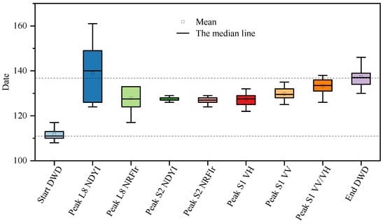
Figure 7.
Comparing the peak flowering dates of rapeseed identified by different indexes with the flowering starts (BBCH61) and ends (BBCH69) observed at DWD stations.
Since the peak flowering dates were not recorded at DWD stations, a strict validation of them retrieved from satellites is impossible [39,62]. Alternatively, the r (Pearson correlation coefficient) and λ (symmetry consistency index) are used to assess the new indexes (NRFIr, VH, VV/VH) by comparing them with the indexes (NDYI and VV) used in a previous study [2] (Figure 8). The L8 NDYI has the most insignificant relationship with other indexes, further confirming its lower ability for identifying peak flowering (Figure 8a). Both NRFIr from L8 and S2 have significant relationships with S2 NDYI and S1 VV. The relationships among both morphological indexes are significant (r ≥ 0.7) (Figure 8a).
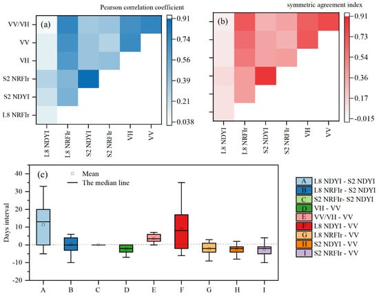
Figure 8.
(a) Pearson correlation coefficients; (b) symmetry consistency indexes; (c) flowering intervals observed from different DWD stations and obtained from the combination of two different indexes.
λ has a very similar pattern to that of r (Figure 8b). For example, there is a quite weak agreement between L8 NDYI and other indexes as indicated by λ, but the highest agreement between S2 NRFIr and S2 NDYI (λ = 0.9). The λ for all morphological indexes (VH, VV/VH, and VV) is >0.7. Thus, NDYI from L8 does not perform as well as NRFIr from L8. Furthermore, VH and VV/VH also can be used to detect the rapeseed peak flowering period.
From the differences in each combination of two indexes for identifying peak flowering dates, we found the largest difference is caused by two NDYI from L8 and S2, with L8 NDYI around 13 days later than that of S2 NDYI (Figure 8c). Also, compared with VV, the peak flowering dates derived from VH is earlier, but those derived from VV/VH have an approximate zero to seven day delay.
4. Discussion
4.1. The Good Performance of NRFI for Identifying Flowering Stages of Rapeseed
In this work, we constructed a novel spectral index—NRFI, which not only shows high sensitivity to rapeseed petals during a vegetation canopy but also easily catches the peak flowering dates. The results show that L8 NRFI outperforms the L8 NDYI in detecting the flowering stages. NRFI is defined as the combination of red band and short-wave infrared band-2 (SWIR2), while NDYI is the combination of green and blue bands. The blue waveband is sensitive to atmospheric contamination and increasing uncertainty in detecting flowering phenology of rapeseed [17]. Moreover, decreasing chlorophyll content of rapeseed petals induces increased reflection in the red waveband [18,35,57]. A decrease in water contents in soil and rapeseed during the flowering period will inevitably be observed by SWIR2 [63,64,65]. Thus, the NRFI developed in our study can unsurprisingly capture such features signature during the time series of the flowering period of rapeseed.
However, previous studies only focused on the visible light waveband (blue, green, and red) and near-infrared waveband. Ignoring the characteristics of short-wave infrared changes (e.g., SWIR2) during rapeseed growth [2,3,5,10,15,17,18,34,38,49]. For example, Siulk et al. [18] designed an index (including green and blue), similar to NDYI, to directly exploit variation in flowering [18]. Plant photosynthesis decreases during rapeseed flowering. They interpreted that the yellowness of rapeseed petals is caused by the carotenoid pigments absorbing the blue light, but reflect a mix of green and red light [17,18].
Besides the above advantages, the NRFI can be further applied to extract the plots cultivated by rapeseed. It has been reported that the phenological features of the crop could be used to identify the planting areas, which has been applied in previous studies although the accuracy varies by locations and methods [20,66]. We analyzed the pixels of NRFIr in the studied areas and find that the NRFIr values of rapeseed during the flowering period are distinctly different from those of other land use types (Figure 9). Comparing with other methods (e.g., visual interpreting of high-resolution images and supervised classifying by machine learning) to extract planting areas, the method based on NRFIr will be a more potential and powerful way since others are either time-consuming or strongly depend on training data collected in fields [2,3,26,27,67]. Therefore, NRFIr has the potential for rapeseed planting area mapping.
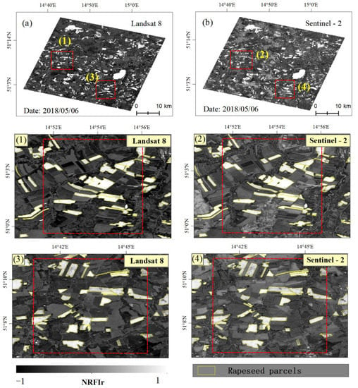
Figure 9.
(a) NRFIr index map from Landsat 8 in the study area; (b) NRFIr index map from Sentinel-2 in the study area; (1)–(4) are partial drawings enlarged.
4.2. The Ancillary Function of Morphological Indexes for Identifying Flowering Stages of Rapeseed
Compared to optical images, SAR images have two advantages: no interruption from clouds and a shorter revisiting cycle. The “V” curves identified by VV and VH from S1 are shown during flowering periods (Figure 6), simultaneously companying with the “reverse V” shapes from optical images (Figure 5). Such changes in both VV and VH are mainly affected by soil and canopy [2,16,68]. For example, VV is particularly sensitive to the water content of vegetation [69]. Rapeseeds’ vertical transformation from a thick rosette of leaves to a flowering stalk will attenuate VV polarization [34]. Moreover, VV and VH increase from the development of fruit to the beginning of ripening because of the rise in the number and the length of stems per plant [2,14,32,34]. Therefore, such changes identified by SAR will be beneficial for characterizing crop phenology features on the other side of optical images [14,19,31]. The “V” changes of VV and VH during the flowering period provide opportunities for an automatic, continuous, and accurate monitoring rapeseed flowering period.
A typical “reverse V” is identified by VV/VH during the rapeseed flowering period (Figure 6), and such changes in VV/VH may be correlated more with fresh biomass than photosynthetic activity [14,30,34]. Additionally, some previous studies have shown that the fresh biomass of wheat and corn is associated with VV/VH [14,34]. Due to the typical changes of VV/VH with the flowering processes, the VV/VH ratio will provide a potential way for applying it for biophysical parameters retrieval into other crops and other regions in the future.
Our findings highlight a highly potential way to detect the flowering stage of rapeseed using SAR data, particularly for VV/VH ratio, which has been rarely investigated in previous studies. Moreover, the characteristic variations in scattering coefficients during rapeseed growth are useful for mapping high-resolution cultivated areas of rapeseed. For example, Singha et al. [68] drew a high-resolution rice map in cloud-prone Bangladesh and Northeast India based on Sentinel-1 SAR backscatter coefficients during rice growth. Additionally, such radar data may also be applied to fill eventual gaps in the optical data series. Following the free availability of Sentinel data, it will eventually support near real-time crop monitoring in the future [14]. Combining SAR with optical data should be more accurate for monitoring the flowering period and planting areas of rapeseed [2,34], which can also be applied to other crops and other regions.
4.3. Limitations and Perspectives
Despite the above findings, the revisit frequency of optical satellite surveys and the number of high-quality images should be considered in characterizing the peak flowering period. Cloud is one of the main limitations in the consistent and accurate detection of flowering phenology of rapeseed. The new method with the indexes proposed in our study will have great potential at high latitudes because of the increasing availability of high-quality images [44,70], especially from Sentinel-1/2 satellites of Europe [58]. Further research should be focused on standardizing a classifier based on the optical and morphological indexes to map in more detail the phenology, growth, and planting areas for rapeseed at a large spatial scale.
5. Conclusions
The Landsat satellite has longer time series historical images and is the main data source for monitoring historical rapeseed flowering phenology. Sentinel-1/2 data have higher temporal and spatial resolutions, which is conducive to monitoring rapeseed phenology accurately. In this study, we integrated Landsat 8 and Sentinel-1/2 data to assess the potential of satellites to detect rapeseed flowering dates. The time series of rapeseed’s reflectance and polarized backscattering coefficients (VH, VV, and VV/VH) were analyzed. The observations collected at different DWD stations were applied. We proposed L8 NRFI and found that it outperforms L8 NDYI in monitoring rapeseed peak flowering. The correlation (r) between L8 NDYI and other indices observed peak flowering dates less than 0.3. L8 NRFIr and other indices were higher correlated (r ≥ 0.5). Also, the results show that VH and VV/VH have the potential to monitor the peak flowering stage of rapeseed. The relationships among both SAR indices are significant (r ≥ 0.7). The VV/VH signals are more pronounced whereas detection by VV/VH is slightly delayed (zero to seven days) relative to VV and VH. The symmetry consistency index (λ) between different indices has a very similar pattern to that of r. The λ for all SAR indexes is ≥0.7. Our study showed that a better understanding of temporal behaviors of spectral indices and backscatters during rapeseed flowering season will benefit not only biophysical parameters monitoring but also dynamic crop growth monitoring and planting area mapping.
Author Contributions
Conceptualization, Z.Z. and J.H.; Data curation, J.H. and J.C.; Methodology, J.H. and Z.Z.; Writing—original draft, J.H.; Writing—review & editing, Z.Z. and J.C. All authors have read and agreed to the published version of the manuscript.
Funding
This study was supported by the National Science Foundation of China (41977405).
Conflicts of Interest
The authors declare that they have no known competing financial interests or personal relationships that could have appeared to influence the work reported in this paper.
Appendix A
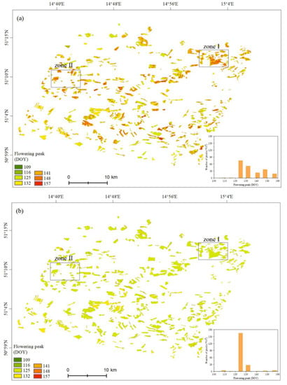
Figure A1.
Flowering peak (Day of Year, DOY) as obtained by (a) NDYI and (b) NRFIr from Landsat-8 images in 2018 in the study area. Histogram depicts the numbers of pixels of rapeseed flowering peak.
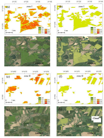
Figure A2.
Zoomed-in images and rapeseed flowering peak (Day of Year, DOY) maps in 2018. The base maps are RGB-composite images using the red, green, and blue bands of the Landsat 8. The zoomed-in regions are Zone Ⅰ and Zone II in Figure A1. Flowering peak as obtained by NDYI (a,e) and NRFIr (b,f). (c,d,g,h) are true color images of different dates and locations.
References
- Gardy, J.; Hassanpour, A.; Lai, X.; Rehan, M. The influence of blending process on the quality of rapeseed oil-used cooking oil biodiesels. Int. Sci. J. (J. Environ. Sci.) 2014, 3, 233–240. [Google Scholar]
- Andrimont, R.; Taymans, M.; Lemoine, G.; Ceglar, A.; Yordanov, M.; van der Velde, M. Detecting flowering phenology in oil seed rape parcels with Sentinel-1 and-2 time series. Remote Sens. Environ. 2020, 239, 111660. [Google Scholar] [CrossRef] [PubMed]
- Tao, J.; Wu, W.; Liu, W.; Xu, M. Exploring the Spatio-Temporal Dynamics of Winter Rape on the Middle Reaches of Yangtze River Valley Using Time-Series MODIS Data. Sustainability 2020, 12, 466. [Google Scholar] [CrossRef]
- Zhang, Y.; Chipanshi, A.; Daneshfar, B.; Koiter, L.; Champagne, C.; Davidson, A.; Reichert, G.; Bédard, F. Effect of using crop specific masks on earth observation based crop yield forecasting across Canada. Remote Sens. Appl. Soc. Environ. 2019, 13, 121–137. [Google Scholar] [CrossRef]
- Domínguez, J.A.; Kumhálová, J.; Novák, P. Winter oilseed rape and winter wheat growth prediction using remote sensing methods. Plant Soil Environ. 2015, 61, 410–416. [Google Scholar]
- Rondanini, D.P.; Gomez, N.V.; Agosti, M.B.; Miralles, D.J. Global trends of rapeseed grain yield stability and rapeseed-to-wheat yield ratio in the last four decades. Eur. J. Agron. 2012, 37, 56–65. [Google Scholar] [CrossRef]
- Ahmadi, M.; Bahrani, M.J. Yield and yield components of rapeseed as influenced by water stress at different growth stages and nitrogen levels. Am. Eurasian J. Agric. Environ. Sci. 2009, 5, 755–761. [Google Scholar]
- Kirkegaard, J.A.; Lilley, J.M.; Brill, R.D.; Ware, A.H.; Walela, C.K. The critical period for yield and quality determination in canola (Brassica napus L.). Field Crop. Res. 2018, 222, 180–188. [Google Scholar] [CrossRef]
- Zhang, H.; Flottmann, S. Source-sink manipulations indicate seed yield in canola is limited by source availability. Eur. J. Agron. 2018, 96, 70–76. [Google Scholar] [CrossRef]
- Behrens, T.; Müller, J.; Diepenbrock, W. Utilization of canopy reflectance to predict properties of oilseed rape (Brassica napus L.) and barley (Hordeum vulgare L.) during ontogenesis. Eur. J. Agron. 2006, 25, 345–355. [Google Scholar] [CrossRef]
- Alqudah, A.M.; Samarah, N.H.; Mullen, R.E. Drought stress effect on crop pollination, seed set, yield and quality. In Alternative Farming Systems, Biotechnology, Drought Stress and Ecological Fertilization; Springer: Berlin/Heidelberg, Germany, 2011; pp. 193–213. [Google Scholar]
- Ashraf, M.; Foolad, M.R. Pre-sowing seed treatment—A shotgun approach to improve germination, plant growth, and crop yield under saline and non-saline conditions. Adv. Agron. 2005, 88, 223–271. [Google Scholar]
- Chen, Y.; Zhang, Z.; Tao, F. Improving regional winter wheat yield estimation through assimilation of phenology and leaf area index from remote sensing data. Eur. J. Agron. 2018, 101, 163–173. [Google Scholar] [CrossRef]
- Veloso, A.; Mermoz, S.; Bouvet, A.; Le Toan, T.; Planells, M.; Dejoux, J.; Ceschia, E. Understanding the temporal behavior of crops using Sentinel-1 and Sentinel-2-like data for agricultural applications. Remote Sens. Environ. 2017, 199, 415–426. [Google Scholar] [CrossRef]
- Tian, H.; Meng, M.; Wu, M.; Niu, Z. Mapping spring canola and spring wheat using Radarsat-2 and Landsat-8 images with Google Earth Engine. Curr. Sci. 2019, 116, 291–298. [Google Scholar] [CrossRef]
- Yang, H.; Li, Z.; Chen, E.; Zhao, C.; Yang, G.; Casa, R.; Pignatti, S.; Feng, Q. Temporal polarimetric behavior of oilseed rape (Brassica napus L.) at C-band for early season sowing date monitoring. Remote Sens. 2014, 6, 10375–10394. [Google Scholar] [CrossRef]
- Sulik, J.J.; Long, D.S. Spectral considerations for modeling yield of canola. Remote Sens. Environ. 2016, 184, 161–174. [Google Scholar] [CrossRef]
- Sulik, J.J.; Long, D.S. Spectral indices for yellow canola flowers. Int. J. Remote Sens. 2015, 36, 2751–2765. [Google Scholar] [CrossRef]
- Bargiel, D. A new method for crop classification combining time series of radar images and crop phenology information. Remote Sens. Environ. 2017, 198, 369–383. [Google Scholar] [CrossRef]
- Luo, Y.; Zhang, Z.; Chen, Y.; Li, Z.; Tao, F. ChinaCropPhen1km: A high-resolution crop phenological dataset for three staple crops in China during 2000–2015 based on leaf area index (LAI) products. Earth Syst. Sci. Data 2020, 12, 197–214. [Google Scholar] [CrossRef]
- Rüetschi, M.; Schaepman, M.E.; Small, D. Using multitemporal sentinel-1 c-band backscatter to monitor phenology and classify deciduous and coniferous forests in northern switzerland. Remote Sens. 2018, 10, 55. [Google Scholar] [CrossRef]
- Van der Meer, F.D.; Van der Werff, H.; Van Ruitenbeek, F. Potential of ESA’s Sentinel-2 for geological applications. Remote Sens. Environ. 2014, 148, 124–133. [Google Scholar] [CrossRef]
- Vermote, E.; Justice, C.; Claverie, M.; Franch, B. Preliminary analysis of the performance of the Landsat 8/OLI land surface reflectance product. Remote Sens. Environ. 2016, 185, 46–56. [Google Scholar] [CrossRef] [PubMed]
- Liu, S.; Liu, X.; Liu, M.; Wu, L.; Ding, C.; Huang, Z. Extraction of rice phenological differences under heavy metal stress using EVI time-series from HJ-1A/B Data. Sensors 2017, 17, 1243. [Google Scholar]
- Magney, T.S.; Eitel, J.U.; Huggins, D.R.; Vierling, L.A. Proximal NDVI derived phenology improves in-season predictions of wheat quantity and quality. Agr. For. Meteorol. 2016, 217, 46–60. [Google Scholar] [CrossRef]
- Griffiths, P.; Nendel, C.; Hostert, P. Intra-annual reflectance composites from Sentinel-2 and Landsat for national-scale crop and land cover mapping. Remote Sens. Environ. 2019, 220, 135–151. [Google Scholar] [CrossRef]
- Preidl, S.; Lange, M.; Doktor, D. Introducing APiC for regionalised land cover mapping on the national scale using Sentinel-2A imagery. Remote Sens. Environ. 2020, 240, 111673. [Google Scholar] [CrossRef]
- Nguyen, D.B.; Gruber, A.; Wagner, W. Mapping rice extent and cropping scheme in the Mekong Delta using Sentinel-1A data. Remote Sens. Lett. 2016, 7, 1209–1218. [Google Scholar] [CrossRef]
- Wang, H.; Magagi, R.; Goïta, K.; Trudel, M.; McNairn, H.; Powers, J. Crop phenology retrieval via polarimetric sar decomposition and random forest algorithm. Remote Sens. Environ. 2019, 231, 111234. [Google Scholar] [CrossRef]
- Betbeder, J.; Fieuzal, R.; Philippets, Y.; Ferro-Famil, L.; Baup, F. Contribution of multitemporal polarimetric synthetic aperture radar data for monitoring winter wheat and rapeseed crops. J. Appl. Remote Sens. 2016, 10, 26020. [Google Scholar] [CrossRef]
- Cable, J.W.; Kovacs, J.M.; Jiao, X.; Shang, J. Agricultural monitoring in northeastern Ontario, Canada, using multi-temporal polarimetric RADARSAT-2 data. Remote Sens. 2014, 6, 2343–2371. [Google Scholar] [CrossRef]
- McNairn, H.; Jiao, X.; Pacheco, A.; Sinha, A.; Tan, W.; Li, Y. Estimating canola phenology using synthetic aperture radar. Remote Sens. Environ. 2018, 219, 196–205. [Google Scholar] [CrossRef]
- Steele-Dunne, S.C.; McNairn, H.; Monsivais-Huertero, A.; Judge, J.; Liu, P.; Papathanassiou, K. Radar remote sensing of agricultural canopies: A review. IEEE J. Stars 2017, 10, 2249–2273. [Google Scholar] [CrossRef]
- Mercier, A.; Betbeder, J.; Baudry, J.; Le Roux, V.; Spicher, F.; Lacoux, J.; Roger, D.; Hubert-Moy, L. Evaluation of Sentinel-1 & 2 time series for predicting wheat and rapeseed phenological stages. ISPRS J. Photogramm. 2020, 163, 231–256. [Google Scholar]
- Pan, Z.; Huang, J.; Wang, F. Multi range spectral feature fitting for hyperspectral imagery in extracting oilseed rape planting area. Int. J. Appl. Earth Obs. 2013, 25, 21–29. [Google Scholar] [CrossRef]
- Wan, L.; Li, Y.; Cen, H.; Zhu, J.; Yin, W.; Wu, W.; Zhu, H.; Sun, D.; Zhou, W.; He, Y. Combining UAV-based vegetation indices and image classification to estimate flower number in oilseed rape. Remote Sens. 2018, 10, 1484. [Google Scholar] [CrossRef]
- Gong, Y.; Duan, B.; Fang, S.; Zhu, R.; Wu, X.; Ma, Y.; Peng, Y. Remote estimation of rapeseed yield with unmanned aerial vehicle (UAV) imaging and spectral mixture analysis. Plant Methods 2018, 14, 70. [Google Scholar] [CrossRef]
- Ashourloo, D.; Shahrabi, H.S.; Azadbakht, M.; Aghighi, H.; Nematollahi, H.; Alimohammadi, A.; Matkan, A.A. Automatic canola mapping using time series of sentinel 2 images. ISPRS J. Photogramm. 2019, 156, 63–76. [Google Scholar] [CrossRef]
- Kaspar, F.; Zimmermann, K.; Polte-Rudolf, C. An overview of the phenological observation network and the phenological database of Germany’s national meteorological service (Deutscher Wetterdienst). Adv. Sci. Res. 2015, 11, 93–99. [Google Scholar] [CrossRef]
- Böttcher, U.; Rampin, E.; Hartmann, K.; Zanetti, F.; Flenet, F.; Morison, M.; Kage, H. A phenological model of winter oilseed rape according to the BBCH scale. Crop Pasture Sci. 2016, 67, 345–358. [Google Scholar] [CrossRef]
- Ma, Y.; Fang, S.; Peng, Y.; Gong, Y.; Wang, D. Remote estimation of biomass in winter oilseed rape (Brassica napus L.) using canopy hyperspectral data at different growth stages. Appl. Sci. 2019, 9, 545. [Google Scholar] [CrossRef]
- She, B.; Huang, J.; Guo, R.; Wang, H.; Wang, J. Assessing winter oilseed rape freeze injury based on Chinese HJ remote sensing data. J. Zhejiang Univ. Sic. B 2015, 16, 131–144. [Google Scholar] [CrossRef] [PubMed]
- Dong, J.; Xiao, X.; Kou, W.; Qin, Y.; Zhang, G.; Li, L.; Jin, C.; Zhou, Y.; Wang, J.; Biradar, C. Tracking the dynamics of paddy rice planting area in 1986–2010 through time series Landsat images and phenology-based algorithms. Remote Sens. Environ. 2015, 160, 99–113. [Google Scholar] [CrossRef]
- Dong, J.; Xiao, X.; Menarguez, M.A.; Zhang, G.; Qin, Y.; Thau, D.; Biradar, C.; Moore, B., III. Mapping paddy rice planting area in northeastern Asia with Landsat 8 images, phenology-based algorithm and Google Earth Engine. Remote Sens. Environ. 2016, 185, 142–154. [Google Scholar] [CrossRef]
- You, N.; Dong, J. Examining earliest identifiable timing of crops using all available Sentinel 1/2 imagery and Google Earth Engine. ISPRS J. Photogramm. 2020, 161, 109–123. [Google Scholar] [CrossRef]
- Foga, S.; Scaramuzza, P.L.; Guo, S.; Zhu, Z.; Dilley Jr, R.D.; Beckmann, T.; Schmidt, G.L.; Dwyer, J.L.; Hughes, M.J.; Laue, B. Cloud detection algorithm comparison and validation for operational Landsat data products. Remote Sens. Environ. 2017, 194, 379–390. [Google Scholar] [CrossRef]
- Torres, R.; Snoeij, P.; Geudtner, D.; Bibby, D.; Davidson, M.; Attema, E.; Potin, P.; Rommen, B.; Floury, N.; Brown, M. GMES Sentinel-1 mission. Remote Sens. Environ. 2012, 120, 9–24. [Google Scholar] [CrossRef]
- Mandal, D.; Kumar, V.; Bhattacharya, A.; Rao, Y.S.; Siqueira, P.; Bera, S. Sen4Rice: A Processing Chain for Differentiating Early and Late Transplanted Rice Using Time-Series Sentinel-1 SAR Data with Google Earth Engine. IEEE Geosci. Remote Sens. 2018, 15, 1947–1951. [Google Scholar] [CrossRef]
- Wang, D.; Fang, S.; Yang, Z.; Wang, L.; Tang, W.; Li, Y.; Tong, C. A regional mapping method for oilseed rape based on HSV transformation and spectral features. ISPRS Int. J. Geo Inf. 2018, 7, 224. [Google Scholar] [CrossRef]
- Mallinis, G.; Mitsopoulos, I.; Chrysafi, I. Evaluating and comparing Sentinel 2A and Landsat-8 Operational Land Imager (OLI) spectral indices for estimating fire severity in a Mediterranean pine ecosystem of Greece. Gisci. Remote Sens. 2018, 55, 1–18. [Google Scholar] [CrossRef]
- Helman, D. Land surface phenology: What do we really ‘see’from space? Sci. Total Environ. 2018, 618, 665–673. [Google Scholar] [CrossRef]
- Geng, L.; Ma, M.; Wang, X.; Yu, W.; Jia, S.; Wang, H. Comparison of eight techniques for reconstructing multi-satellite sensor time-series NDVI data sets in the Heihe river basin, China. Remote Sens. 2014, 6, 2024–2049. [Google Scholar] [CrossRef]
- Wang, C.; Zhang, Z.; Chen, Y.; Tao, F.; Zhang, J.; Zhang, W. Comparing different smoothing methods to detect double-cropping rice phenology based on LAI products–a case study in the Hunan province of China. Int. J. Remote Sens. 2018, 39, 6405–6428. [Google Scholar] [CrossRef]
- Eklundh, L.; Jönsson, P. TIMESAT 3.1 Software Manual; Lund University: Lund, Sweden, 2012; pp. 1–82. [Google Scholar]
- Benesty, J.; Chen, J.; Huang, Y.; Cohen, I. Pearson correlation coefficient. In Noise Reduction in Speech Processing; Springer: Berlin/Heidelberg, Germany, 2009; pp. 1–4. [Google Scholar]
- Duveiller, G.; Fasbender, D.; Meroni, M. Revisiting the concept of a symmetric index of agreement for continuous datasets. Sci. Rep. UK 2016, 6, 1–14. [Google Scholar] [CrossRef] [PubMed]
- Shen, M.; Chen, J.; Zhu, X.; Tang, Y. Yellow flowers can decrease NDVI and EVI values: Evidence from a field experiment in an alpine meadow. Can. J. Remote Sens. 2009, 35, 99–106. [Google Scholar] [CrossRef]
- Drusch, M.; Del Bello, U.; Carlier, S.; Colin, O.; Fernandez, V.; Gascon, F.; Hoersch, B.; Isola, C.; Laberinti, P.; Martimort, P. Sentinel-2: ESA’s optical high-resolution mission for GMES operational services. Remote Sens. Environ. 2012, 120, 25–36. [Google Scholar] [CrossRef]
- Roy, D.P.; Wulder, M.A.; Loveland, T.R.; Woodcock, C.E.; Allen, R.G.; Anderson, M.C.; Helder, D.; Irons, J.R.; Johnson, D.M.; Kennedy, R. Landsat-8: Science and product vision for terrestrial global change research. Remote Sens. Environ. 2014, 145, 154–172. [Google Scholar] [CrossRef]
- Wiseman, G.; McNairn, H.; Homayouni, S.; Shang, J. RADARSAT-2 polarimetric SAR response to crop biomass for agricultural production monitoring. IEEE J. Stars 2014, 7, 4461–4471. [Google Scholar] [CrossRef]
- Vreugdenhil, M.; Wagner, W.; Bauer-Marschallinger, B.; Pfeil, I.; Teubner, I.; Rüdiger, C.; Strauss, P. Sensitivity of Sentinel-1 backscatter to vegetation dynamics: An Austrian case study. Remote Sens. 2018, 10, 1396. [Google Scholar] [CrossRef]
- van Vliet, A.J.H.; de Groot, R.S.; Bellens, Y.; Braun, P.; Bruegger, R.; Bruns, E.; Clevers, J.; Estreguil, C.; Flechsig, M.; Jeanneret, F.; et al. The European Phenology Network. Int. J. Biometeorol. 2003, 47, 202–212. [Google Scholar] [CrossRef]
- Chen, D.; Huang, J.; Jackson, T.J. Vegetation water content estimation for corn and soybeans using spectral indices derived from MODIS near-and short-wave infrared bands. Remote Sens. Environ. 2005, 98, 225–236. [Google Scholar] [CrossRef]
- Seelig, H.D.; Hoehn, A.; Stodieck, L.S.; Klaus, D.M.; Adams Iii, W.W.; Emery, W.J. The assessment of leaf water content using leaf reflectance ratios in the visible, near-, and short-wave-infrared. Int. J. Remote Sens. 2008, 29, 3701–3713. [Google Scholar] [CrossRef]
- Wilson, R.H.; Nadeau, K.P.; Jaworski, F.B.; Tromberg, B.J.; Durkin, A.J. Review of short-wave infrared spectroscopy and imaging methods for biological tissue characterization. J. Biomed. Opt. 2015, 20, 30901. [Google Scholar] [CrossRef] [PubMed]
- Luo, Y.; Zhang, Z.; Li, Z.; Chen, Y.; Zhang, L.; Cao, J.; Tao, F. Identifying the spatiotemporal changes of annual harvesting areas for three staple crops in China by integrating multi-data sources. Environ. Res. Lett. 2020, 15, 74003. [Google Scholar] [CrossRef]
- Wesołowski, M.; Suchacz, B. Classification of rapeseed and soybean oils by use of unsupervised pattern-recognition methods and neural networks. Fresenius J. Anal. Chem. 2001, 371, 323–330. [Google Scholar] [CrossRef]
- Singha, M.; Dong, J.; Zhang, G.; Xiao, X. High resolution paddy rice maps in cloud-prone Bangladesh and Northeast India using Sentinel-1 data. Sci. Data 2019, 6, 1–10. [Google Scholar] [CrossRef]
- Cookmartin, G.; Saich, P.; Quegan, S.; Cordey, R.; Burgess-Allen, P.; Sowter, A. Modeling microwave interactions with crops and comparison with ERS-2 SAR observations. IEEE Trans. Geosci. Remote 2000, 38, 658–670. [Google Scholar] [CrossRef]
- Zhou, Y.; Dong, J.; Liu, J.; Metternicht, G.; Shen, W.; You, N.; Zhao, G.; Xiao, X. Are There Sufficient Landsat Observations for Retrospective and Continuous Monitoring of Land Cover Changes in China? Remote Sens. 2019, 11, 1808. [Google Scholar] [CrossRef]
Publisher’s Note: MDPI stays neutral with regard to jurisdictional claims in published maps and institutional affiliations. |
© 2020 by the authors. Licensee MDPI, Basel, Switzerland. This article is an open access article distributed under the terms and conditions of the Creative Commons Attribution (CC BY) license (http://creativecommons.org/licenses/by/4.0/).