Article

Integration of Remotely Sensed Soil Sealing Data in Landslide Susceptibility Mapping

1
Dipartimento di Scienze della Terra, Università degli Studi di Firenze, Via La Pira 4, 50121 Firenze, Italy
2
ISPRA-Italian Institute for Environmental Protection and Research, Via Brancati 48, 00144 Rome, Italy
*
Author to whom correspondence should be addressed.
Remote Sens. 2020, 12(9), 1486; https://doi.org/10.3390/rs12091486
Submission received: 28 March 2020 / Revised: 5 May 2020 / Accepted: 6 May 2020 / Published: 7 May 2020
(This article belongs to the Special Issue Remote Sensing for Disaster Risk Management)

Abstract

:
Soil sealing is the destruction or covering of natural soils by totally or partially impermeable artificial material. ISPRA (Italian Institute for Environmental Protection Research) uses different remote sensing techniques to monitor this process and updates yearly a national-scale soil sealing map of Italy. In this work, for the first time, we tried to combine soil sealing indicators as additional parameters within a landslide susceptibility assessment. Four new parameters were derived from the raw soil sealing map: Soil sealing aggregation (percentage of sealed soil within each mapping unit), soil sealing (categorical variable expressing if a mapping unit is mainly natural or sealed), urbanization (categorical variable subdividing each unit into natural, semi-urbanized, or urbanized), and roads (expressing the road network disturbance). These parameters were integrated with a set of well-established explanatory variables in a random forest landslide susceptibility model and different configurations were tested: Without the proposed soil-sealing-derived variables, with all of them contemporarily, and with each of them separately. Results were compared in terms of AUC ((area under receiver operating characteristics curve, expressing the overall effectiveness of each configuration) and out-of-bag-error (estimating the relative importance of each variable). We found that the parameter “soil sealing aggregation” significantly enhanced the model performances. The results highlight the potential relevance of using soil sealing maps on landslide hazard assessment procedures.

Graphical Abstract

1. Introduction

Landslide susceptibility mapping (LSM) is the representation of the spatial probability of landslide occurrence, based on the correlation between known landslide locations and the spatial arrangement of a set of predisposing factors [1,2]. The scientific literature is rich in different methodologies to produce LSM [3], ranging from simple bivariate statistical methods like the frequency ratio [4,5,6], logistic regression [7,8], discriminant analysis [9], weight of evidence [10,11], and favorability functions [4], to complex machine learning algorithms like artificial neural networks [12,13], random forest [14,15,16], and ensembles or hybrid combinations of any two methods [17,18,19,20].
Of course, besides the statistical techniques used to perform the susceptibility assessment, the input data are also very important, as their selection, number, and parameterization can largely influence the quality of the results [14,21,22]. Several authors pointed out that geographic information systems (GISs) can be useful tools to prepare the input data and to run the LSM [23,24] and the challenge to increase the quality, accuracy, and areal coverage of many input data has led to wide use of remote sensing techniques [25,26,27,28].
For instance, satellite missions provide world-coverage digital elevation models (DEMs) with increasing resolution and accuracy that can be imported in a GIS and used to derive morphometric parameters (such as the slope gradient, curvature, aspect, terrain roughness, and so on), which are used in landslide medium-scale susceptibility studies. Conversely, in local-scale applications, high-resolution DEMs can be obtained using LiDAR (Light Detection And Ranging) [29]. Another series of remotely sensed products, which are widely used in LSM, are indicators of the vegetation cover (e.g., the NDVI – Normalized Difference Vegetation Index) [30,31] and land-use or land-cover thematic maps [22,32,33].
Concerning land cover data, for years, the Corine Land Cover (CLC) dataset has represented the standard reference for complete and homogeneous mapping in Europe. The CLC consists of an inventory of 44 land cover classes, with a minimum mapping unit of 25 hectares. With the purpose of providing a sort of monitoring of land cover dynamics, several updates have been released, the first one in 1990 and the last one in 2018. CLC data can be accessed and used freely (https://land.copernicus.eu/pan-european/corine-land-cover). For this reason, CLC is commonly used as an input variable in LSM in Europe, especially in small-scale applications [32,34]. Despite the undoubtful usefulness of CLC data in LSM and geographical studies in general, the classification system and the spatial resolution prevent an optimal use in very detailed analysis. For example, [22], in a 1.10,000 scale LSM study located in France, showed that better results can be obtained using land cover maps purposely developed by means of photointerpretation. Similarly, in more general environmental applications, it was demonstrated that the analysis of land cover changes using CLC data or other land-use maps did not allow precise evaluation of the soil sealing rate, especially in rural areas of Italy [35,36]. Furthermore, in the artificial surface classes, fragmented areas and sparse houses are underestimated, thus leading to a systematic underestimation of soil consumption and soil sealing [36].
Soil sealing can be defined as the destruction or covering of soils by buildings, constructions, and layers of completely or partly impermeable artificial material (asphalt, concrete, etc.). It is the most intense form of land take and is essentially an irreversible process [37]. Land consumption can be defined as the variation from a natural soil (or land not consumed) to an artificial land cover (land consumed), where land cover is the observed (bio)physical cover on the Earth’s surface, including artificial surfaces, agricultural areas, woods and forests, semi-natural areas, wetlands, and water bodies [37]. The most typical representation of land consumption is given by the growing set of areas covered by buildings, constructions, paved or unpaved roads, quarries, landfills, construction sites, courtyards, yards, and other paved or clay-paved areas, etc.
As part of its activities, ISPRA (Italian Institute for Environmental Protection and Research) is undertaking several activities related to land cover monitoring to assess land consumption evolution over the last few decades in Italy. In collaboration with the network of regional environmental agencies, ISPRA realizes each year a high-resolution (10 m) layer that identifies the sealed and artificial coverage areas for the entire Italian territory [38].
The connection between hydro-geomorphological hazards and soil sealing/land consumption is widely acknowledged: The latter can completely change the hydrological system of hillslopes and catchments, leading to an increase in runoff rates, a reduction of lag time during storms, and a concentration of water in correspondence with human artifacts [39,40,41]. Moreover, a poor design or insufficient maintenance of buildings and infrastructures located on hillslopes and mountainsides may be directly related to an increase of landslide hazards [42,43,44]. However, to our knowledge, a statistical correlation between soil sealing and landslide susceptibility has never been attempted. Therefore, the primary objective of this work was to investigate whether the soil sealing data from the ISPRA monitoring program can be integrated into a landslide susceptibility model. To this aim, different input parameters were derived from the raw soil sealing data and tested as explanatory variables. Their contribution in the modeling was quantitatively evaluated to define which parameter is the most useful to improve landslide susceptibility assessments.

2. Materials and Methods
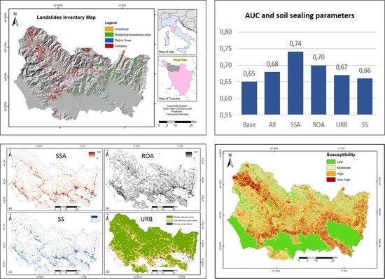
2.1. Study Area

The study area covers an area of 3100 km2 located in the northern part of the Tuscany region, Italy as Figure 1 shows. The area was chosen because of the availability of several high-quality datasets and because it is very prone to landslides [45].
According to traditional studies [46,47] and to the most recently updated landslide inventories (which were obtained by combining geomorphological fieldwork, photointerpretation, and satellite remote sensing) [48,49], the main landslide types affecting the area can be classified as slides (rotational, translational, and compound), slow earth flows, complex movements (mainly slides evolving into flows), and, to a lesser extent, debris flows (see also the landslide dataset description in Section 2.3). The main triggering factor is rainfall, with mean annual precipitations gradually ranging from about 1000 mm/year in the plains to about 1900 mm/year in the western mountains [50]. The area is characterized by a high energy of relief, with the steep slopes of the Apennines mountains grading from the maximum altitude of about 2000 m a.s.l. to low-altitude narrow intermontane tectonic valleys or to the floor of a wide alluvial plain with an altitude close to 0 m a.s.l. From a lithological point of view, the bedrock of the area is mainly composed of layered flysch rocks and by metamorphic rocks (phyllite and schists) [46], which play a significant role as landslide-predisposing factors [21]. The mountains are covered by forests and are sparsely urbanized, and the main villages and cities are located in the valley floors and in the surrounding hills. The sectors of the area occupied by wide alluvial plains were excluded from the analyses because landslides are not a geomorphological process that occurs in a similar setting.

2.2. Random Forest Algorithm

The random forest (RF) algorithm, originally proposed by [51], is a machine learning technique based on the binary decision tree classification model. The RF algorithm performs a random sampling of the observations included in the training dataset to create binary decision trees in which a random selection of the explanatory variables is used to split each node (yes/no) and to perform a classification. The observations excluded from the sampling (called “out-of-bag”) are used for internal evaluation of the prediction trees and to adjust the definition of the trees generated in other iterations of the process, with the aim of minimizing the prediction errors. Indeed, a single random tree would have a very low predictive capability; thus, to get stable results and lower errors, this application requires the use of several (typically hundreds) randomly generated trees, hence the name “random forest”. Usually, in RF applications, a sub-dataset is excluded from the analyses and exclusively used as an independent dataset to validate the results obtained with the optimal “forest” defined by the model.
An interesting feature of RF is the internal procedure of weighting of variables: The out-of-bag samples are used to calculate the prediction error (out-of-bag error) that would be committed if a variable were excluded from the modeling. In this way, the RF algorithm can be used to get, at the same time, a susceptibility mapping, validation of its predictive accuracy, and a study on the sensitivity of the results to the explanatory variables used in the model.
RF can be used to solve classification and regression problems and it is a well-established technique in LSM because it is very flexible [14,16,52]: It can use, at the same time, categorical and continuous numerical variables, it can exploit complex information provided by many variables, it can handle multicollinearity, and it is relatively robust with respect to overfitting issues.

2.3. Basic Input Data

The landslides location was obtained from IFFI (Inventory of landslides in Italy), a nation-wide catalogue of landslides published by ISPRA, which aims to provide an overview of the distribution of landslides throughout the country and to provide a basic cognitive tool for assessing landslide hazards [53]. It contains 620,808 landslides for a total area of 23,700 km2 (7.9% of the Italian territory). Landslides are mapped at the 1:10,000 scale and are classified according to [54]. A total of 7799 landslides with areal extension ranging from 102 to 106 m2 were identified in the study area: Most of them are mapped as complex movements (typically rotational/translational slides evolving into slow earthflows) (55%) or as rotational/translational slides (35%) (Figure 2). Following the same approach used in previous works, the susceptibility analysis considers only these two typologies. This assumption is supported by two main reasons: First, the triggering mechanism and causative factors are the same; second, the distinction between the two typologies in the inventory is often uncertain and may depend on the interpretation of the surveyors [21,48,49]. Debris flows (4%) and landslides with unspecified typology of movement (6%) were excluded from the analysis.
In our application, we decided to work at a 100-m spatial resolution, since this mesoscale has been acknowledged to be a good compromise in regional-scale landslide susceptibility studies [14,55]. Many landslides included in the inventory have dimensions smaller than this cell size, and their significance is taken into account following a methodology of analysis introduced by [14,34]: The dependent variable to be modeled is not represented by a binary classification scheme (pixel with landslides—pixel without landslides), but it is a continuous variable ranging from 0 to 100 and expressing the area of the mapping unit interested in by landslides. When coarse spatial units are used, this approach allows all landslides (and clusters of landslides) to have a significance weighted by their dimensions. Consequently, the 7799 selected landslides were combined with a grid of the area (with 100 m × 100 m cell size), and for each cell, the percentage of territory covered by landslides was calculated and used as the dependent variable for the landslide susceptibility assessment.
The production of a landslide susceptibility map requires the knowledge of the spatial distribution and interactions of various explanatory variables, which allow landslide-prone areas to be defined. There is no consensus about which is the optimal set of explanatory variables to be used in susceptibility studies and probably an optimal set is something very relative as it may vary according to the landslide type, to the characteristics of the study area, and to the characteristics (e.g., spatial resolution or scale) of the available datasets. However, the main objective of this study was not to produce the best possible susceptibility map but to explore the possibility of using a new explanatory variable derived from soil sealing monitoring data. As a consequence, a very limited set of parameters was used to define the base configuration of the susceptibility model: The “base parameters” were selected among the most used according to a literature review of general landslide studies [3] and studies focused on the same test site [14,56,57]. The base parameters are reported and briefly presented in Table 1.

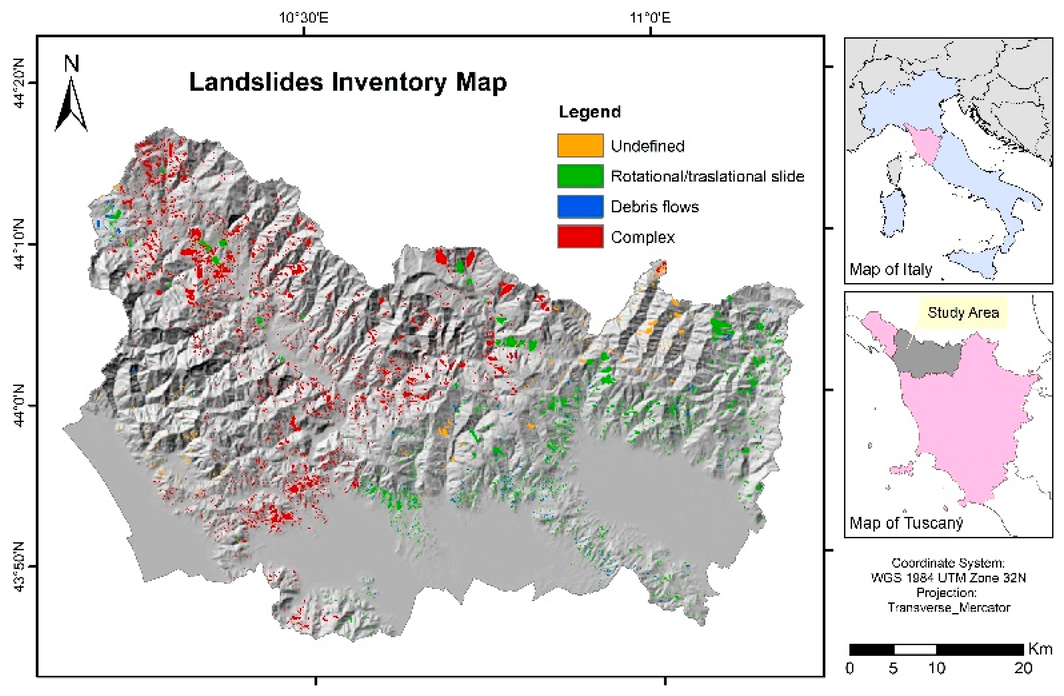
2.4. Soil Sealing Raw Data

Since soil sealing data were the focal point of the research, this paragraph contains a brief description of the ISPRA soil sealing dataset, together with an overview of the methodology that was developed for producing it. Since 2015, ISPRA has undertaken a national-scale monitoring program of land cover and one of the delivered products is a national cartography of soil sealing in the raster format (pixel size 10*10 m), in which the whole Italian territory is classified into two classes: Sealed soil/not sealed soil. The monitoring activity includes an update of this product every year. In this study, we employed the map updated to the year 2017.
In the year 2015, the first soil sealing map was generated by using RapidEye images [58,59], which consist of 5 bands (blue, green, red, NIR – Near Infra-Red, and red edge) at a 5-m spatial resolution [58]. The map was obtained by supervised classification with the maximum likelihood; to increase the accuracy of classification, ancillary data and intensive manual photointerpretation of Very High Resolution (VHR) images and national orthophotos were also used [60].
After 2015, the soil sealing map was updated yearly at a 10-m spatial resolution. A new methodology was implemented to update the soil sealing map each year and to exploit the potential of both Sentinel 2 optical and Sentinel 1 radar satellites. The methodology includes some of the main steps described below.
The new soil sealing mapping procedure was based on Sentinel-2 images because they ensure the best spatial and spectral resolution among the freely available optical images in Italy. The Sentinel-2 images can be used for both photointerpretation and semi-automatic classification purposes. The multispectral instrument (MSI) of Sentinel-2 provides 13 bands from visible to short wave infrared (SWIR) with a 10-m, 20-m, and 60-m resolution, depending on the spectral band (Table 2). The three 60-m bands (b1, b9, and b10) were not used in the procedure, due to their coarse spatial resolution.
The geometric data resolution was aligned for all image datasets, in order to ensure the consistency of mapping on an annual basis, throughout all the available Copernicus datasets. The Sentinel-2 images were corrected to account for distortions caused by atmosphere and terrain morphology, in order to derive a preliminary thematic classification layer that distinguishes natural soils from imperviousness areas. This first rough classification was improved through specific elaborations based on spectral vegetation indexes that are useful for the detection of target land cover classes. Some masks were created by exploiting the maximum NDVI values calculated over the image time series. These values highlight vegetated areas, and, by contrast, mask the non-vegetated areas (such as sealed land, bare soil, bare rocks, and so on). The maximum NDVI (pixel based) of the current year was compared to the maximum NDVI of the previous year and differences were calculated on a pixel-by-pixel basis; changes were acknowledged if the differences were greater than a set of thresholds empirically calibrated during the last years [60,61], i.e., the difference was higher than 0.2 and the NDVI value of the current year was lower than 0.3 (absence of vegetation). This method allowed identification of the areas where vegetation is removed or is greatly diminished.
Another type of analysis was carried out by exploiting the key features of the Sentinel-1 ground range-detected (GRD) data product, including 20-m spatial resolution with a pixel spacing of 10 m and availability of dual polarization acquisitions (VV and VH). Dual polarization acquisitions are widely used for monitoring urban areas, since different polarizations have different sensitivities and different backscattering coefficients for the same target [62]. The first-level image classification obtained from Sentinel-2 classification was integrated by the Sentinel 1 information. The VV polarization is particularly useful to detect land cover changes. The median of the VV values of the Sentinel-1 acquisition of the current year was compared to the median of VV of the previous year: If the difference was greater than 0.1 dB and the median of the current year was lower than −9 dB (i.e., buildings have low VV values), the pixel was considered a possible change due to the construction of buildings.
The output of this integration represents a second-level soil sealing map that represents the base for a following work of manual photointerpretation on multitemporal VHR images and orthophotos for the whole Italian territory on a detailed scale (≥1:5000). In this way, it is possible to accurately (spatial resolution of 0.5 m) detect the limits of the area concerned, to identify the type of change that occurred, and finally, to perform a binary classification encompassing sealed vs. not sealed soil classes. Sealed soils include built-up areas, paved roads, railways, airports, ports, and other paved areas (public squares, parking lots, courtyards, sport fields, permanent paved greenhouses). They also include reversible land consumption: Dirt roads, construction sites, and other compacted earth areas. A further validation process was then performed by using very high-resolution orthophotos and Google Earth imagery as control datasets.
After the classification process was finished, an accuracy analysis was performed by selecting a random sample of control points and calculating accuracy indexes. Finally, the final soil sealing map was re-projected in the ETRS_1989_LAEA system and made available in a public repository (http://groupware.sinanet.isprambiente.it/uso-copertura-e-consumo-di-suolo/library/consumo-di-suolo).

2.5. Soil Sealing Parameterization for Landslide Susceptibility Mapping

This study aimed to investigate whether soil sealing data can be effectively used in landslide susceptibility mapping models. To this aim, the soil sealing map released by ISPRA (see previous section) was used as raw data to derive some parameters to be tested as explanatory variables in landslide susceptibility assessments. Indeed, the original soil sealing map contains very basic information (dichotomic classification between sealed and not-sealed soil) at high spatial resolution (10 m) and some alternate approaches may be needed to convert this information into continuous variables, or to aggregate it at different pixel sizes. The tested parameters were “soil sealing”, “urbanization”, “soil sealing aggregation” (percentage of sealed soil), and “roads”; they are briefly introduced hereafter and are shown in Figure 3.

2.5.1. Soil Sealing (SS)

This parameter is the most similar to the original soil sealing data: Since the original raw data consists of a raster at a 10-m resolution in which each cell represents sealed vs. non-sealed soil, this layer was downsampled in the GIS environment to a 100-m resolution by using the “majority” operator. At the end of the process, each cell represented a portion of territory, where most of the area is occupied either by artificial structures or by natural and semi-natural soil. This parameter was included in the tests because it represents the result of the most straightforward method to assimilate the soil sealing raw data to the mapping unit defined for an application.

2.5.2. Urbanization (URB)

This parameter represents the density of urbanization: It was derived from the original high-resolution soil sealing map, after a re-classification in three classes:
  • Predominantly natural areas;
  • Low-density urbanized areas; and
  • Predominantly artificial areas, with a high density of urbanization
The identification of urban density was carried out on high-resolution soil sealing data with the “focal statistics” tool of ArcMap 10.6, assigning to each pixel the mean value of all the pixels present in a circular area of a 600-m radius. The result was reclassified in three classes, whose limits were defined by comparison with the Copernicus Urban Atlas data set.

2.5.3. Soil Sealing Aggregation (SSA)

This variable was calculated by using the soil sealing layer at a 10-m resolution; a data aggregation operation was performed in a GIS environment and the output was a raster with a 100-m cell size, where the value expresses the number of sealed 10-m-resolution cells. This dataset therefore presents a range of integer values from 0 to 100, which could also be interpreted as the percentage of soil sealed within each hectare. In other applications involving different pixel sizes, a simple arithmetical operation should be performed to convert the count of sealed cells into a percentage.

2.5.4. Roads (ROA)

The distance to roads is traditionally considered as one of the most important anthropogenic factors influencing landslides and it is widely used in landslide susceptibility studies [3]. Roads are included in the raw soil sealing maps but are not distinguishable from other sealing factors. Consequently, to isolate the contribution of the road network to the generalized soil sealing process, OpenStreetMap (in vector format with line geometry) was used. From the original layer, the main and secondary communication routes were selected; only the small mountain tracks were not considered. A 10-m buffer was created around the lines representing the roads to define an area of disturbance, then the resulting polygons were rasterized and aggregated to a resolution of 100 m. As a final check, ROA and SSA raster were compared: Since the former systematically had lower values than the latter, we are confident that ROA can be considered a subset of the aggregated soil sealing map, where the contribution of roads is isolated from other soil sealing processes.

2.6. Description of the Landslide Susceptibility Tests

To train the susceptibility model, 15,557 randomly selected points were considered. The constraints for the random selection were set as follows: Half of them were randomly sampled within landslide areas, the other half were sampled in areas outside landslide polygons. Even if some studies use crowns, scarps, or detachment zones to sample landslide conditions, we took into account the whole landslide polygon (typically encompassing both the detachment zone and accumulation zone), because the landslides of the area are often subject to reactivations and therefore, in the landslide susceptibility assessment, the definition of conditions associated to landslide bodies that could be reactivated is as important as the definition of conditions associated to new activations. Moreover, the use of the whole landslide area was necessary because, as explained in Section 2.3, the dependent variable is defined as the area of each cell occupied by landslides and consists of a continuous value that will be modeled with a regression (while most of the literature studies perform a classification on binary instances of presence of landsides vs. the absence of landslides). The dataset was divided in a 70% subsample for model training and a 30% subsample for independent verification and testing. Within the subsamples, the balance between landslide and non-landslide conditions was kept at 50%–50%.
The susceptibility assessment was performed in regression mode using a graphical user interface (GUI) developed in MATLAB, derived from a previous work [63] and already used in several applications to produce and validate landslide susceptibility maps and to investigate the forecasting effectiveness of each input parameter [21,63]. The validation of the susceptibility assessment was performed in terms of AUC (area under receiver-operator characteristic curves), a quantitative index widely used in landslide susceptibility studies to quantify the overall predictive effectiveness of a model [3,64,65]. AUC is a cutoff-independent index with an operating range from 0.5 (completely random predictions) to 1.0 (perfection) [65]. The relative importance of each parameter used within a model configuration is quantitatively expressed by the OOBE (out of bag error), an estimation of the relative error that the model would commit if a given parameter were omitted (as for the procedure described in Section 2.2).
According to sensitivity analyses performed in previous studies [14], the random forest model was tuned by using 200 trees and by performing for each configuration 20 different runs to handle the randomness of the results provided by the RF approach. Therefore, the AUC and OOBE values are intended as mean values of the results obtained in each of the 20 iterations.
A series of tests was conceived to assess whether soil sealing can provide a useful contribution in landslide susceptibility mapping and which soil sealing parameterization provides the best outcomes. The first test was performed using only the basic parameters (base configuration), while a second test was carried out using all the basic parameters together with all the soil sealing parameters. The first test allowed analysis of the performance of the model in a basic and standard configuration, establishing a benchmark for further comparisons with other sets of input parameters. The second one allowed calculation of the relative importance of each variable when all of them were considered together: The objective of this test was to have a direct comparison of the importance of all the parameters, as expressed in terms of OOBE values.
The last group of tests was carried out by adding to the base configuration each time a single soil-sealing-derived variable. For each configuration, the mean and maximum AUC were calculated, and the relative importance of each variable was defined in terms of OOBE.

3. Results

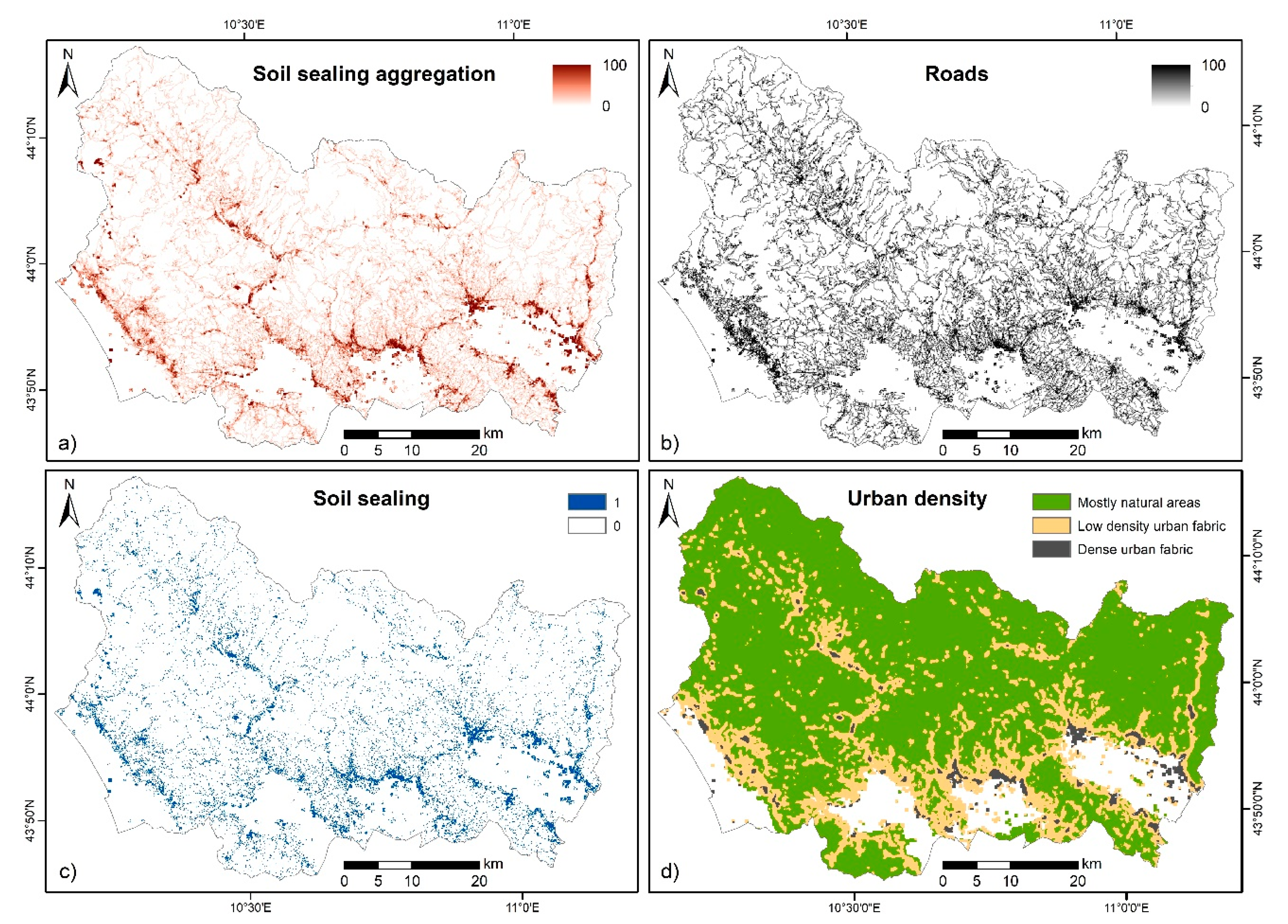
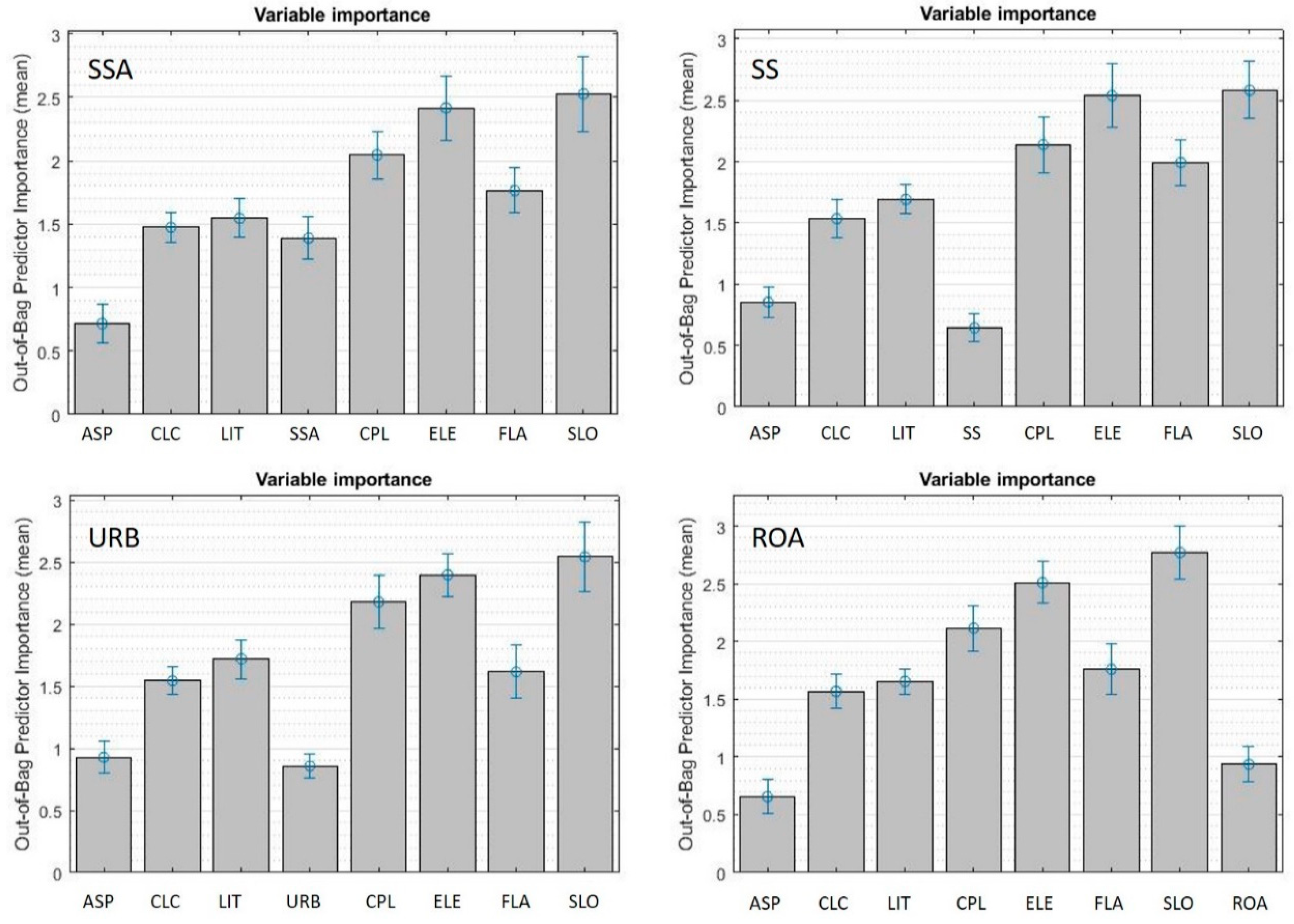
3.1. Sensitivity to Soil Sealing Parameterization

The first objective of the tests was to investigate the sensitivity of the susceptibility assessment to different parameterizations of soil sealing information. To this aim, the AUC values obtained by the validation of the different model configurations were compared and used as an indicator of their accuracy. Figure 4 shows that the base configuration used as a benchmark reports the lowest accuracy (AUC = 0.65), thus indicating that soil sealing information has the potential to improve the accuracy of the susceptibility assessments. However, the results are very sensitive to the different parameterizations of soil sealing information: Some of the soil sealing-derived parameters produce only a very limited improvement of the model (SS, URB), while others bring a more marked contribution (ROA, SSA). The joint use of all the variables together returns intermediate results. The configuration that returned the best validation statistics is the one using the soil sealing aggregation (SSA) parameter, with an AUC of 0.74, showing that land consumption can be used as an important feature in landslide susceptibility mapping.
Another outcome of the test that can be used to investigate the impact of soil sealing-derived parameters in the landslide susceptibility assessment is the comparison of OOBE values, which are indicators of the relative importance of each variable used. Figure 5 shows that the relative importance of the main morphometrical parameters does not vary significantly from a configuration to another: Slope gradient, elevation, curvature, and flow accumulation are the most important parameters, followed by the categorical variables “lithology” and “land cover”. The soil sealing-derived parameters have a ranking (and a relative importance) that is clearly connected to the quality of the results observed with the AUC: The most effective parameter (SSA) has an OOBE value very close to lithology and land cover and markedly higher than the variable “aspect”. The parameter accounting for roads (ROA) has a ranking higher than aspect but the OOBE is lower than CLC and lithology. The other two soil sealing-derived parameters are ranked as the least important parameters (yet with a positive impact on the modelling), and this is reflected by the low AUC values of the derived susceptibility assessments (which are, however, slightly higher than the base configuration) (Figure 4). The results expressed in terms of AUC values and OOBE rankings are consistent and point out that soil sealing aggregation (SSA), at least in this case of study, is the most effective way to improve a landslide susceptibility assessment with soil sealing. Therefore, this parameterization was selected as a benchmark for the subsequent analyses.

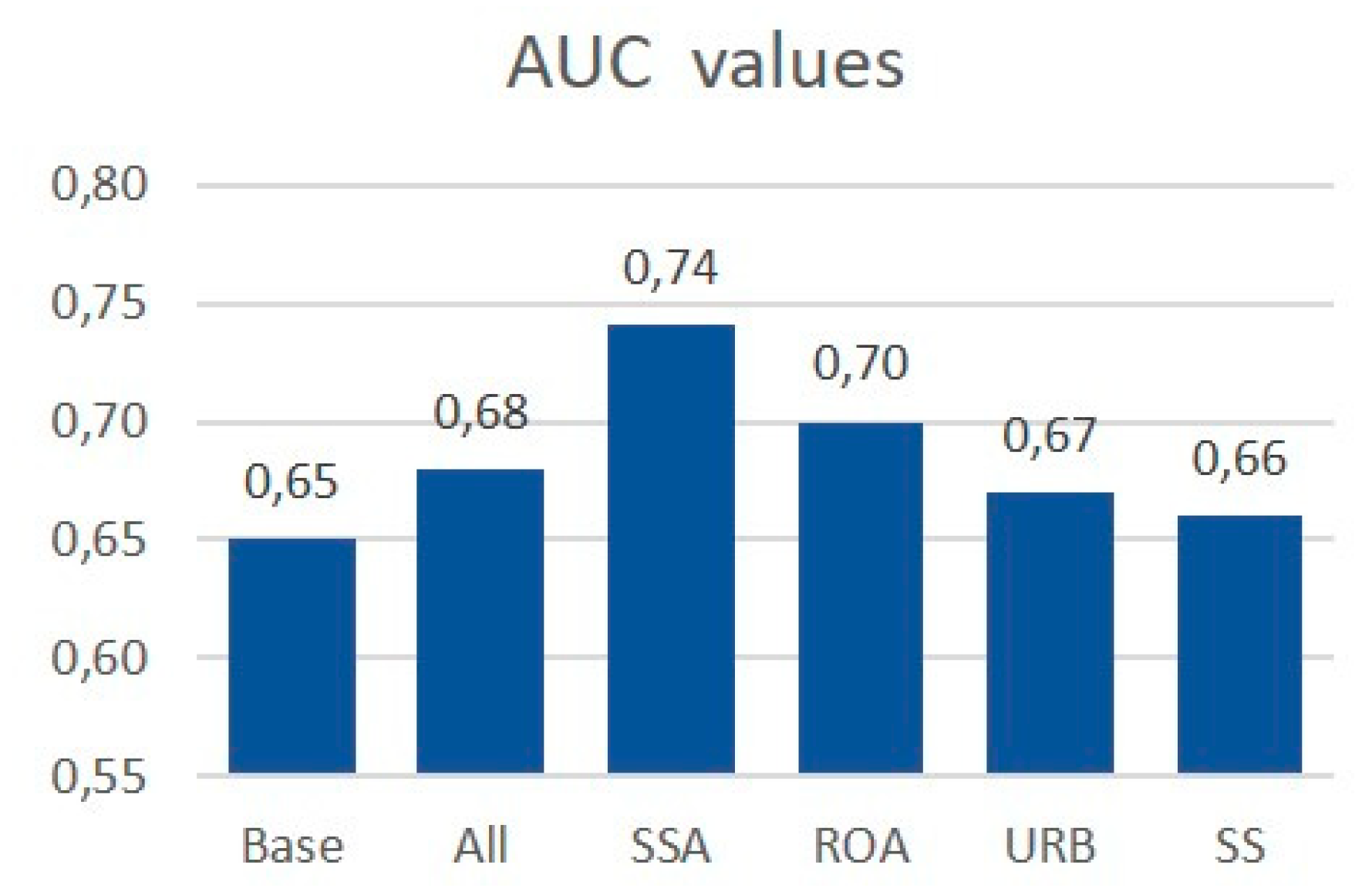
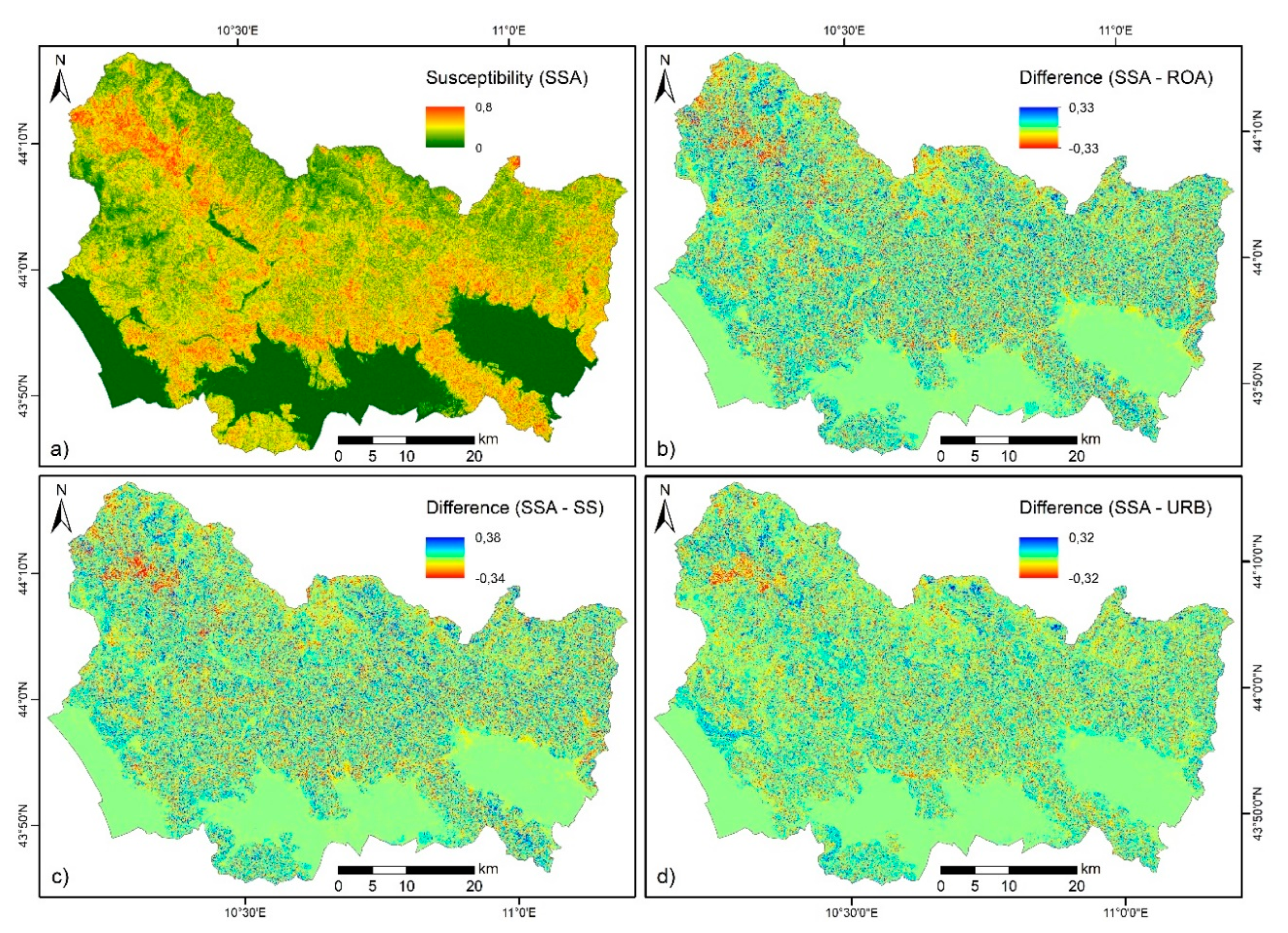
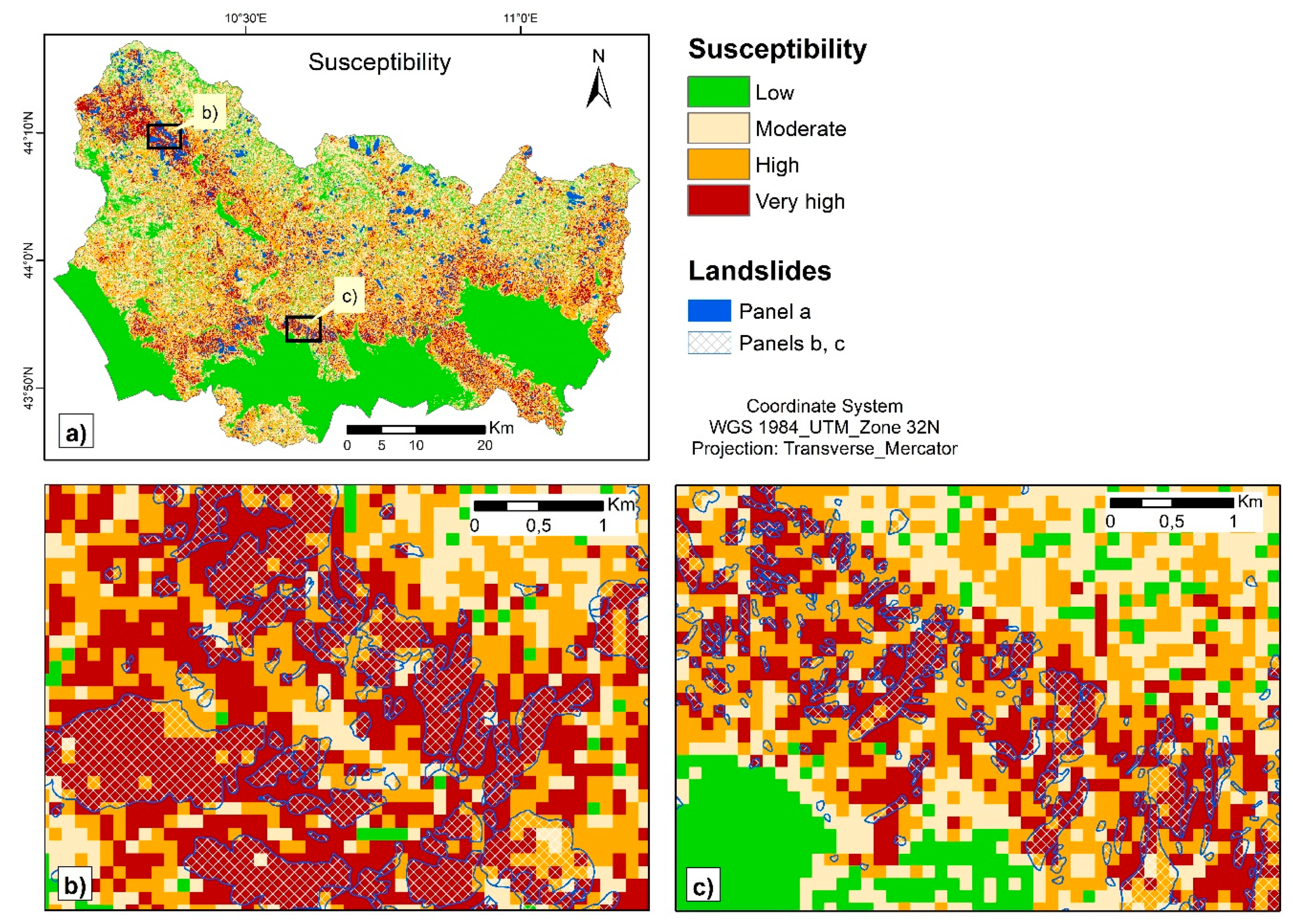
3.2. Susceptibility Mapping

Figure 6a shows the susceptibility map obtained by using the best configuration (the one including the parameter “soil sealing aggregation”). Following an approach proposed by [16], the other susceptibility assessments were represented in terms of deviation from the benchmark map: Using a GIS system, the susceptibility maps obtained using ROA, SS, and URB were subtracted from the SSA map. Figure 6b,c,d show the differences, on a pixel-by-pixel basis, in the modelled susceptibility values. In some points, the differences are relevant (maximum overestimation is 0.38 and maximum underestimation is −0.34, as shown in Table 3, but they never reach “extreme values”, as defined by [16]. Moreover, Figure 6 shows that except for an area in the NW sector of the test site, where the SSA-derived susceptibility is generally lower than the others, underestimations and overestimations do not have a systematic spatial pattern: They are not concentrated in some precise zones and they have a “salt and pepper” distribution.
For completeness, a reclassified susceptibility map of the area obtained with the SSA configuration is shown in Figure 7. According to the Italian national regulation on landslide hazards, the susceptibility values were divided into four qualitative classes. To this aim, the well-established [15,66] Jenks method based on natural breaks was used, as it is an objective approach to optimize the data clustering by reducing the variance within classes while maximizing the variance between classes. According to this classification, low susceptibility zones occupy 32% of the study area and moderate, high, and very high zones occupy 32%, 27%, and 10%, respectively (Figure 7a).

4. Discussion

The outcomes of the analyses demonstrated that soil sealing information can have a positive influence in regional-scale landslide susceptibility assessments, but the results are sensitive to the approach used to parametrize soil sealing. Since in Italy soil sealing raw data are characterized by a very fine spatial resolution (10-m pixels) and coarse information (dichotomous classification in sealed and not-sealed pixels), the application to susceptibility models based on wider spatial units requires the derivation of parameters and many approaches could be pursued. In this study, we introduced, tested, and compared four approaches based on four different soil sealing-derived variables.
The best model configuration corresponds to the one that uses the soil sealing aggregation variable, with an AUC value of 0.74 and a higher ranking and OOBE value than other soil sealing-derived parameters. Among the tested variables, SSA includes the most detailed information, with continuous values ranging from 0 to 100 representing the degree of sealing (and thus the degree of anthropogenic “disturbance”) in each 100m * 100m cell used as the spatial unit in the susceptibility analysis. It is worth highlighting that to create this variable, the pixel size was upscaled from 10 (the native resolution of the raw soil sealing map) to 100m, but despite the coarser spatial resolution, the SSA variable had a positive effect in the susceptibility assessment. Indeed, the OOBE is relatively high (similar to other important variables as lithology and land cover) and the derived susceptibility map has an overall accuracy higher than the base configuration.
This outcome is important as it leaves open other possibilities of application with different spatial units like basins or geomorphic units, which, although less common [3], are receiving growing attention [17,67,68].
The configuration encompassing SSA is the only one that returned an AUC higher than 0.70, which is used by some authors as the limit to “good” results [69]. Indeed, in the susceptibility mapping literature, it is common to find even higher AUC values, but the main objective of this work was to assess the sensitivity to soil sealing parameterization and identify some promising parameters derived by ISPRA soil sealing monitoring products. For this reason, only a few morphological and thematic parameters have been used as explanatory variables of the susceptibility model, to avoid that the impact of shadowing of the soil sealing-derived features. It is not excluded that other scholars could use the SSA parameter inside a more complex susceptibility model and to get better results in terms of AUC. For instance, other authors in the same test site obtained an AUC of 0.84 by using a random forest model with 23 explanatory variables [56]. However, even if the SSA-derived map can surely be ameliorated, a fair match between the susceptibility map and the landslide polygons can be observed in several sectors of the area (Figure 7b,c).
By using the same soil sealing raw data, two other similar parameters were defined, but they returned worst results. Among all the variables created, SS is conceptually the most similar to the original raw data: The territory is classified in the same two classes (natural soil or sealed soil) and the only difference is the downsampling from the original cell size of 10m to the resolution used in the susceptibility assessment (100m). However, there are two main limitations that in our opinion negatively influenced the results on landslide susceptibility mapping, making the SS parameter irrelevant. First, the rescaling procedure brought a loss of spatial detail (spatial resolution is one of the main advantages of the raw soil sealing maps). Second, some uncertainties were added as the “majority” operator used to aggregate pixels from 10 to 100m is not able to represent intermediate situations in which the 100-m cell is only partially sealed. To overcome the latter limitation, the URB parameter was conceived: It basically reflects the SS structure, but it also has an intermediate class to account for partially sealed spatial units. However, the improvement in terms of AUC and OOBE is very limited and leads to poor results.
The second-best result was given by the roads, with an AUC of 0.70 and a higher ranking and OOBE than SS and URB. ROA was structured as a continuous variable ranging from 0 to 1, each cell representing the percentage of area occupied by roads of every typology, from large highways to small paved roads. Conceptually, ROA is a subset of SSA: While the former quantifies the disturbance of roads on the hillslope system, the latter quantifies the disturbance driven by every human structure. Relative to the susceptibility mapping, in our case of study, SSA seems to be more significant than ROA and to foster better results. This outcome should not be surprising, since roads are widely acknowledged as one of the most important human-related landslide-predisposing factors, especially when built with cut-and-fill techniques. Indeed, the same can also apply to every other human asset, including buildings, as pointed out by a growing number of examples in the literature [70,71,72]. From this perspective, the use of road network is clearly only partial information, while a good (i.e., spatially accurate and timely updated) soil sealing map, like the ones produced every year by ISPRA in Italy, has the potential to hold more complete information that can be conveniently used in landslide susceptibility mapping. Regarding landslides influenced by road networks or other constructions, it should be stressed that in this area, they are quite frequent but have typically small sizes [45,48,50,53]. Despite the relatively coarse (100m x 100m) cell size, the modeling approach allows proper consideration to be given to both large and small landslides, because the modeled susceptibility index represents the percentage of landslide area expected in the mapping unit.
Another important test is the one using all soil sealing-related parameters altogether (“ALL” model configuration). The random forest technique is acknowledged to be able to handle many parameters even if they are partially correlated and to avoid collinearity issues. However, the joint use of SSA, SS, URB, and ROA does not provide satisfactory results (AUC = 0.68). This is in contrast with other similar applications, e.g., [21] in the same test site demonstrated that a landslide susceptibility assessment can be improved if many thematic maps with slightly different geological meanings are jointly used. In the present case of study, the four different parameters derived from soil sealing raw data are evidently redundant and the best prediction was obtained when only the best of them (SSA) was used alone. This outcome can be interpreted as further evidence of the effectiveness of SSA.
In many scientific papers about landslide susceptibility, land cover maps are used as input variables, and their influence on the results is widely recognized. This was confirmed by our results, since land cover has a positive influence on the susceptibility assessment. However, it is important to remark that land cover was outperformed by soil sealing aggregation (higher ranking and OOBE value). Although Corine Land Cover presents good thematic detail, it is less effective in spatial resolution (25 hectares minimum mappable unit) than soil sealing thematic maps, and this is probably the main reason of the lower forecasting effectiveness. In particular, the spatial resolution of CLC is ineffective in mapping the Italian soil sealing phenomenon, which has peculiar spatial characteristics: As [38] clearly pointed out, its spatial pattern is typically fragmented, and small roads and urban sprawl areas are systematically underestimated or even ignored. The fact that a better parameterization of urban fabric leads to an improved accuracy of the derived LSM could be considered as further evidence of the importance of human drivers on landslide activity, at least in this study area. Consequently, the possibility of using land consumption to improve landslide susceptibility assessments brings two advantages: A fine spatial resolution of 10 m of the raw data and a good temporal resolution, as the soil sealing thematic layers in Italy and in other European countries are updated on an annual frequency. The latter point is particularly important also from the perspective of providing timely updates of landslide hazard assessments.
As a last point of discussion, some comparisons could be made with other susceptibility assessments already performed in the same test site [21,56]. Both works describe an RF-based modeling approach that is very similar to the one used in the present work; thus, the differences can be considered depending mainly on the use of explanatory variables. Initially, [56] attempted to draw a first susceptibility map of the area, resorting to 23 state-of-the-art explanatory variables. The resulting map was validated, and a 0.84 AUC value was obtained. More recently, [21] used the same area to optimize the parameterization of geological information in the landslide susceptibility assessment. They used as a benchmark a reduced base configuration of parameters (similar to the one used in this article), then improved the modeling by adding complex and multifaceted geological information in the susceptibility model [21]. The AUC values of the resulting maps were improved from 0.60 to 0.75. The AUC improvement was similar to the one observed in this study (from 0.65 to 0.74). In light of these observations, the present work provided some preliminary insights on the possibility to use in LSM activities a new parameter derived from nation-wide soil sealing monitoring programs. When sensitivity analyses and further tests are carried out for other variables as well, the gained knowledge will be summarized in a new and improved comprehensive LSM effort, in the framework of future research activities on this area.

5. Conclusions

Soil sealing maps at a 10-m spatial resolution covering the whole Italian territory are updated every year by ISPRA. In this work, this high-resolution thematic layer was used for the first time in a landslide susceptibility assessment. The test site was a 3100-km2 area located in northern Tuscany (Italy), with 7799 observed landslides, mostly rotational, translational, and compound landslide types. Four different variables were derived from the soil sealing raw data: Soil sealing aggregation (SSA—a continuous variable expressing the percentage of sealed soil within the selected mapping unit), soil sealing (SS—a dichotomous categorical variable expressing if a given mapping unit is composed of natural soil or sealed soil), urbanization (URB—a categorical variable subdividing each unit into natural, seminatural, or urbanized soil), and road (ROA—similar to SSA but encompassing only the effect of road network instead of all human structures).
The main objective of this research was to use these four soil sealing variables and test if they could improve the accuracy of landslide susceptibility assessments. A random forest algorithm was used for the susceptibility analysis and seven conditioning factors were used as base variables (aspect, land cover, slope, elevation, lithology, planar curvature, and flow accumulation). The four soil sealing-derived variables were integrated in the susceptibility model, resulting in a series of tests (each variable alone, all variables together, none of them). For each test, the overall accuracy of the resulting map was evaluated in terms of AUC; in addition, the importance of each variable was evaluated in terms of the “out of bag error”.
The results showed that:
  • Soil sealing data can be used to improve the effectiveness of landslide susceptibility assessments;
  • Among the tested variables, “soil sealing aggregation” was the most promising, leading to the highest AUC and showing a relative importance within the model higher than other widely used parameters like land cover;
  • In addition to the improved forecasting effectiveness, the use of soil sealing-derived parameters in landslide susceptibility studies seems promising because the original thematic layer is updated yearly, and this good temporal resolution allows for a quick and constant update of susceptibility maps accounting for the modifications induced by human activity on hillslope systems; and
  • All the proposed variables were formulated in general terms to make their use reproducible in other susceptibilities studies, even in those based on spatial units different from those used here. The methodology is technically reproducible in Italy and in all other countries with similar environmental monitoring programs.

Author Contributions

Conceptualization, S.S.; methodology, S.S, T.L. and F.C.; software, F.C.; validation, T.L. and S.S; investigation, T.L and S.S.; writing—original draft preparation, S.S and T.L.; writing—review and editing, T.L., S.S, M.M. and F.C.; visualization, T.L.; supervision, M.M., N.C.; funding acquisition, N.C. All authors have read and agreed to the published version of the manuscript.

Funding

This work was funded by “Dipartimento della Protezione Civile – Presidenza del Consiglio dei Ministri” (Presidency of the Council of Ministers - Department of Civil Protection); this publication, however, does not reflect the position and official policies of the Department.

Acknowledgments

This work was also supported by Università degli Studi di Firenze in the framework of the project SEGONISAMUELERICATEN20.

Conflicts of Interest

The authors declare no conflict of interest.

References

  1. Corominas, J.; Copons, R.; Vilaplana, J.M.; Altimir, J.; Amigó, J. Integrated landslide susceptibility analysis and hazard assessment in the principality of Andorra. Nat. Hazards 2003, 30, 421–435. [Google Scholar] [CrossRef]
  2. Fell, R.; Corominas, J.; Bonnard, C.; Cascini, L.; Leroi, E.; Savage, W.Z. Guidelines for landslide susceptibility, hazard and risk zoning for land use planning. Eng. Geo. 2008, 102, 85–98. [Google Scholar] [CrossRef] [Green Version]
  3. Reichenbach, P.; Rossi, M.; Malamud, B.D.; Mihir, M.; Guzzetti, F. A review of statistically-based landslide susceptibility models. Earth Sci. Rev. 2018, 180, 60–91. [Google Scholar] [CrossRef]
  4. Chung, C.F.; Fabbri, A.G. Validation of spatial prediction models for landslide hazard mapping. Nat. Hazards 2003, 30, 451–472. [Google Scholar] [CrossRef]
  5. Yilmaz, I. Landslide susceptibility mapping using frequency ratio, logistic regression, artificial neural networks and their comparison: A case study from Kat landslides (Tokat-Turkey). Comput. Geosci. UK 2009, 35, 1125–1138. [Google Scholar] [CrossRef]
  6. Kavoura, K.; Sabatakakis, N. Investigating landslide susceptibility procedures in Greece. Landslides 2019, 17, 127–145. [Google Scholar] [CrossRef]
  7. Manzo, G.; Tofani, V.; Segoni, S.; Battistini, A.; Catani, F. GIS techniques for regional-scale landslide susceptibility assessment: The Sicily (Italy) case study. Int. J. Geogr. Inf. Sci. 2013, 27, 1433–1452. [Google Scholar] [CrossRef]
  8. Melo, R.; Zêzere, J.L.; Rocha, J.; Oliveira, S.C. Combining data-driven models to assess susceptibility of shallow slides failure and run-out. Landslides 2019, 16, 2259–2276. [Google Scholar] [CrossRef]
  9. Carrara, A. Multivariate models for landslide hazard evaluation. Math. Geol. 1983, 15, 403–426. [Google Scholar] [CrossRef]
  10. Ilia, I.; Tsangaratos, P. Applying weight of evidence method and sensitivity analysis to produce a landslide susceptibility map. Landslides 2016, 13, 379–397. [Google Scholar] [CrossRef]
  11. Thiery, Y.; Malet, J.P.; Sterlacchini, S.; Puissant, A.; Maquaire, O. Landslide susceptibility assessment by bivariate methods at large scales: Application to a complex mountainous environment. Geomorphology 2007, 92, 38–59. [Google Scholar] [CrossRef] [Green Version]
  12. Lee, S.; Ryu, J.-H.; Won, J.-S.; Park, H.-J. Determination and application of the weights for landslide susceptibility mapping using an artificial neural network. Eng. Geol. 2004, 71, 289–302. [Google Scholar] [CrossRef]
  13. Ermini, L.; Catani, F.; Casagli, N. Artificial neural networks applied to landslide susceptibility assessment. Geomorphology 2005, 66, 327–343. [Google Scholar] [CrossRef]
  14. Catani, F.; Lagomarsino, D.; Segoni, S.; Tofani, V. Landslide susceptibility estimation by random forests technique: Sensitivity and scaling issues. Nat. Hazards Earth Syst. Sci. 2013, 13, 2815–2831. [Google Scholar] [CrossRef] [Green Version]
  15. Youssef, A.M.; Pourghasemi, H.R.; Pourtaghi, Z.S.; Al-Katheeri, M.M. Landslide susceptibility mapping using random forest, boosted regression tree, classification and regression tree, and general linear models and comparison of their performance at Wadi Tayyah basin, Asir region, Saudi Arabia. Landslides 2016, 13, 839–856. [Google Scholar] [CrossRef]
  16. Xiao, T.; Segoni, S.; Chen, L.; Yin, K.; Casagli, N. A step beyond landslide susceptibility maps: A simple method to investigate and explain the different outcomes obtained by different approaches. Landslides 2019, 17, 627–640. [Google Scholar] [CrossRef] [Green Version]
  17. Rossi, M.; Guzzetti, F.; Reichenbach, P.; Mondini, A.C.; Peruccacci, S. Optimal landslide susceptibility zonation based on multiple forecasts. Geomorphology 2010, 114, 129–142. [Google Scholar] [CrossRef]
  18. Shirzadi, A.; Bui, D.T.; Pham, B.T.; Solaimani, K.; Chapi, K.; Kavian, A.; Shahabi, H.; Revhaug, I. Shallow landslide susceptibility assessment using a novel hybrid intelligence approach. Environ. Earth Sci. 2017, 76, 60. [Google Scholar] [CrossRef]
  19. Dou, J.; Yunus, A.P.; Bui, D.T.; Merghadi, A.; Sahana, M.; Zhu, Z.; Chen, C.-W.; Han, Z.; Pham, B.T. Improved landslide assessment using support vector machine with bagging, boosting, and stacking ensemble machine learning framework in a mountainous watershed, Japan. Landslides 2020, 17, 641–658. [Google Scholar] [CrossRef]
  20. Yang, Y.; Yang, J.; Xu, C.; Xu, C.; Song, C. Local-scale landslide susceptibility mapping using the B-GeoSVC model. Landslides 2019, 16, 1301–1312. [Google Scholar] [CrossRef]
  21. Segoni, S.; Pappafico, G.; Luti, T.; Catani, F. Landslide susceptibility assessment in complex geological settings: Sensitivity to geological information and insights on its parameterization. Landslides 2020, 1–11. [Google Scholar] [CrossRef] [Green Version]
  22. Fressard, M.; Thiery, Y.; Maquaire, O. Which data for quantitative landslide susceptibility mapping at operational scale? Case study of the Pays d’Auge plateau hillslopes (Normandy, France). Nat. Hazards Earth Syst. Sci. 2014, 14, 569–588. [Google Scholar] [CrossRef] [Green Version]
  23. Süzen, M.L.; Doyuran, V. A comparison of the GIS based landslide susceptibility assessment methods: Multivariate versus bivariate. Environ. Geol. 2004, 45, 665–679. [Google Scholar] [CrossRef]
  24. Ayalew, L.; Yamagishi, H. The application of GIS-based logistic regression for landslide susceptibility mapping in the Kakuda-Yahiko mountains, central Japan. Geomorphology 2005, 65, 15–31. [Google Scholar] [CrossRef]
  25. Sarkar, S.; Kanungo, D.P. An integrated approach for landslide susceptibility mapping using remote sensing and GIS. Photogramm. Eng. Remote Sens. 2004, 70, 617–625. [Google Scholar] [CrossRef]
  26. Lee, S. Application of logistic regression model and its validation for landslide susceptibility mapping using GIS and remote sensing data. Int. J. Remote Sens. 2005, 26, 1477–1491. [Google Scholar] [CrossRef]
  27. Hong, Y.; Adler, R.; Huffman, G. Use of satellite remote sensing data in the mapping of global landslide susceptibility. Nat. Hazards 2007, 43, 245–256. [Google Scholar] [CrossRef] [Green Version]
  28. Park, N.W.; Chi, K.H. Quantitative assessment of landslide susceptibility using high-resolution remote sensing data and a generalized additive model. Int. J. Remote Sens. 2008, 29, 247–264. [Google Scholar] [CrossRef]
  29. Jebur, M.N.; Pradhan, B.; Tehrany, M.S. Optimization of landslide conditioning factors using very high-resolution airborne laser scanning (LiDAR) data at catchment scale. Remote Sens. Environ. 2014, 152, 150–165. [Google Scholar] [CrossRef]
  30. Pradhan, B.; Sezer, E.A.; Gokceoglu, C.; Buchroithner, M.F. Landslide susceptibility mapping by neuro-fuzzy approach in a landslide-prone area (Cameron Highlands, Malaysia). IEEE Trans. Geosci. Remote Sens. 2010, 48, 4164–4177. [Google Scholar] [CrossRef]
  31. Sezer, E.A.; Pradhan, B.; Gokceoglu, C. Manifestation of an adaptive neuro-fuzzy model on landslide susceptibility mapping: Klang valley, Malaysia. Expert Syst. Appl. 2011, 38, 8208–8219. [Google Scholar] [CrossRef]
  32. Bălteanu, D.; Chendeş, V.; Sima, M.; Enciu, P. A country-wide spatial assessment of landslide susceptibility in Romania. Geomorphology 2010, 124, 102–112. [Google Scholar] [CrossRef]
  33. Shu, H.; Hürlimann, M.; Molowny-Horas, R.; González, M.; Pinyol, J.; Abancó, C.; Ma, J. Relation between land cover and landslide susceptibility in Val d’Aran, Pyrenees (Spain): Historical aspects, present situation and forward prediction. Sci. Total Environ. 2019, 693, 133557. [Google Scholar] [CrossRef]
  34. Trigila, A.; Frattini, P.; Casagli, N.; Catani, F.; Crosta, G.; Esposito, C.; Iadanza, C.; Lagomarsino, D.; Scarascia Mugnozza, G.; Segoni, S.; et al. Landslide susceptibility mapping at national scale: The Italian case study. In Landslide Sciences Practice; Margottini, C., Canuti, P., Sassa, K., Eds.; Springer: Berlin/Heidelberg, Germany, 2013; Volume 1, pp. 287–295. [Google Scholar]
  35. Maricchiolo, C.; Sambucini, V.; Pugliese, A.; Munafò, M.; Cecchi, G.; Rusco, E.; Blasi, C.; Marchetti, M.; Chirici, G.; Corona, P. La Realizzazione in Italia del Progetto Europeo CLC2000; APAT Rapporti: Roma, Italy, 2005; pp. 1–86. [Google Scholar]
  36. Munafò, M.; Salvati, L.; Zitti, M. Estimating soil sealing rate at national level—Italy as a case study. Ecol. Indic. 2013, 26, 137–140. [Google Scholar] [CrossRef]
  37. Prokop, G.; Jobstmann, H.; Schöbauer, A. Overview on Best Practices for Limiting Soil Sealing and Mitigating Its Effects in EU-27; European Communities: Brussels, Belgium, 2011. [Google Scholar] [CrossRef]
  38. Munafò, M. Consumo di Suolo, Dinamiche Territoriali e Servizi Ecosistemici; SNPA: Rome, Italy, 2019; p. 224. [Google Scholar]
  39. Chen, L.; Sela, S.; Svoray, T.; Assouline, S. The role of soil-surface sealing, microtopography, and vegetation patches in rainfall-runoff processes in semiarid areas. Water Resour. Res. 2013, 49, 5585–5599. [Google Scholar] [CrossRef]
  40. Pistocchi, A. Hydrological impact of soil sealing and urban land take. In Urban Expansion, Land Cover and Soil Ecosystem Services, 1st ed.; Gardi, C., Ed.; Routledge: London, UK, 2017; pp. 157–168. [Google Scholar]
  41. Acquaotta, F.; Faccini, F.; Fratianni, S.; Paliaga, G.; Sacchini, A.; Vilímek, V. Increased flash flooding in genoa metropolitan area: A combination of climate changes and soil consumption. Meteorl. Atmos. Phys. 2019, 131, 1099–1110. [Google Scholar] [CrossRef]
  42. Martino, S.; Bozzano, F.; Caporossi, P.; D’Angiò, D.; Della Seta, M.; Esposito, C.; Fantini, A.; Fiorucci, M.; Giannini, L.M.; Iannucci, R.; et al. Impact of landslides on transportation routes during the 2016–2017 central Italy seismic sequence. Landslides 2019, 16, 1221–1241. [Google Scholar] [CrossRef]
  43. Dikshit, A.; Sarkar, R.; Pradhan, B.; Segoni, S.; Alamri, A.M. Rainfall induced landslide studies in Indian Himalayan region: A critical review. Appl. Sci. 2020, 10, 2466. [Google Scholar] [CrossRef] [Green Version]
  44. Collins, T.K. Debris flows caused by failure of fill slopes: Early detection, warning, and loss prevention. Landslides 2008, 5, 107–120. [Google Scholar] [CrossRef]
  45. Battistini, A.; Rosi, A.; Segoni, S.; Lagomarsino, D.; Catani, F.; Casagli, N. Validation of landslide hazard models using a semantic engine on online news. Appl. Geogr. 2017, 82, 59–65. [Google Scholar] [CrossRef]
  46. Carmignani, L.; Conti, P.; Cornamusini, G.; Pirro, A. Geological map of Tuscany (Italy). J. Maps 2013, 9, 487–497. [Google Scholar] [CrossRef]
  47. Casagli, N.; Dapporto, S.; Ibsen, M.L.; Tofani, V.; Vannocci, P. Analysis of the landslide triggering mechanism during the storm of 20th–21st November 2000, in northern Tuscany. Landslides 2006, 3, 13–21. [Google Scholar] [CrossRef]
  48. Rosi, A.; Tofani, V.; Tanteri, L.; Stefanelli, C.T.; Agostini, A.; Catani, F.; Casagli, N. The new landslide inventory of Tuscany (Italy) updated with PS-InSAR: Geomorphological features and landslide distribution. Landslides 2018, 15, 5–19. [Google Scholar] [CrossRef] [Green Version]
  49. Bianchini, S.; Raspini, F.; Solari, L.; Del Soldato, M.; Ciampalini, A.; Rosi, A.; Casagli, N. From picture to movie: Twenty years of ground deformation recording over Tuscany region (Italy) with satellite InSAR. Front. Earth Sci. 2018, 6, 177. [Google Scholar] [CrossRef] [Green Version]
  50. Segoni, S.; Rossi, G.; Rosi, A.; Catani, F. Landslides triggered by rainfall: A semi-automated procedure to define consistent intensity-duration thresholds. Comput. Geosci. UK 2014, 63, 123–131. [Google Scholar] [CrossRef]
  51. Breiman, L. Random forests. Mach. Learn. 2001, 45, 5–32. [Google Scholar] [CrossRef] [Green Version]
  52. Brenning, A. Spatial prediction models for landslide hazards: Review, comparison and evaluation. Nat. Hazards Earth Syst. Sci. 2005, 5, 853–862. [Google Scholar] [CrossRef]
  53. Trigila, A.; Iadanza, C.; Spizzichino, D. Quality assessment of the Italian landslide inventory using GIS processing. Landslides 2010, 7, 455–470. [Google Scholar] [CrossRef]
  54. Cruden, D.M.; Varnes, D.J. Landslide types and processes. In Landslide Investigation and Mitigation (Transportation Research Board, National Research Council); Turner, A.K., Schuster, R.L., Eds.; Transportation Research Board National Academy Press: Washington, DC, USA, 1996; Volume 247, pp. 36–75. [Google Scholar]
  55. Chacón, J.; Irigaray, C.; Fernández, T.; El Hamdouni, R. Engineering geology maps: Landslides and geographical information systems. Bull. Eng. Geol. Environ. 2006, 65, 341–411. [Google Scholar] [CrossRef]
  56. Segoni, S.; Tofani, V.; Lagomarsino, D.; Moretti, S. Landslide susceptibility of the Prato-Pistoia-Lucca provinces, Tuscany, Italy. J. Maps. 2016, 12, 401–406. [Google Scholar] [CrossRef] [Green Version]
  57. Segoni, S.; Tofani, V.; Rosi, R.; Catani, F.; Casagli, N. Combination of rainfall thresholds and susceptibility maps for dynamic landslide hazard assessment at regional scale. Front. Earth Sci. 2018, 6, 85. [Google Scholar] [CrossRef] [Green Version]
  58. Tigges, J.; Lakes, T.; Hostert, P. Urban vegetation classification: Benefits of multitemporal RapidEye satellite data. Remote Sens. Environ. 2013, 136, 66–75. [Google Scholar] [CrossRef]
  59. Munafò, M. Il Consumo di Suolo in Italia; SNPA: Rome, Italy, 2015; p. 90. [Google Scholar]
  60. Jiménez-Muñoz, J.C.; Sobrino, J.A.; Gillespie, A.; Sabol, D.; Gustafson, W.T. Improved land surface emissivities over agricultural areas using ASTER NDVI. Remote Sens. Environ. 2006, 103, 474–487. [Google Scholar] [CrossRef]
  61. Neinavaz, E.; Skidmore, A.K.; Darvishzadeh, R. Effects of prediction accuracy of the proportion of vegetation cover on land surface emissivity and temperature using the NDVI threshold method. Int. J. Appl. Earth. Obs. 2020, 85, 101984. [Google Scholar] [CrossRef]
  62. Matsuoka, M.; Yamazaki, F. Use of satellite SAR intensity imagery for detecting building areas damaged due to earthquakes. Earthq. Spectra 2004, 20, 975–994. [Google Scholar] [CrossRef]
  63. Lagomarsino, D.; Tofani, V.; Segoni, S.; Catani, F.; Casagli, N. A tool for classification and regression using random forest methodology: Applications to landslide susceptibility mapping and soil thickness modeling. Environ. Model Assess. 2017, 22, 201–214. [Google Scholar] [CrossRef]
  64. Fawcett, T. An introduction to ROC analysis. Pattern Recognit. Lett. 2006, 27, 861–874. [Google Scholar] [CrossRef]
  65. Frattini, P.; Crosta, G.; Carrara, A. Techniques for evaluating the performance of landslide susceptibility models. Eng. Geol. 2010, 111, 62–72. [Google Scholar] [CrossRef]
  66. Aleotti, P.; Chowdhury, R. Landslide hazard assessment: Summary review and new perspectives. Bull. Eng. Geol. Environ. 1999, 58, 21–44. [Google Scholar] [CrossRef]
  67. Van den Eeckhaut, M.; Reichenbach, P.; Guzzetti, F.; Rossi, M.; Poesen, J. Combined landslide inventory and susceptibility assessment based on different mapping units: An example from the Flemish Ardennes, Belgium. Nat. Hazards Earth Syst. Sci. 2009, 9, 507–521. [Google Scholar] [CrossRef] [Green Version]
  68. Alvioli, M.; Marchesini, I.; Reichenbach, P.; Rossi, M.; Ardizzone, F.; Fiorucci, F.; Guzzetti, F. Automatic delineation of geomorphological slope units with r.slopeunits v1.0 and their optimization for landslide susceptibility modeling. Geosci. Model Dev. 2016, 9, 3975–3991. [Google Scholar] [CrossRef] [Green Version]
  69. Arabameri, A.; Rezaei, K.; Cerdà, A.; Conoscenti, C.; Kalantari, Z. A comparison of statistical methods and multi-criteria decision making to map flood hazard susceptibility in Northern Iran. Sci. Total Environ. 2019, 660, 443–458. [Google Scholar] [CrossRef] [PubMed]
  70. Zhang, F.; Liu, G.; Chen, W.; Liang, S.; Chen, R.; Han, W. Human-induced landslide on a high cut slope: A case of repeated failures due to multi-excavation. J. Rock Mech. Geotech. Eng. 2012, 4, 367–374. [Google Scholar] [CrossRef]
  71. Notti, D.; Galve, J.P.; Mateos, R.M.; Monserrat, O.; Lamas-Fernández, F.; Fernández-Chacón, F.; Roldán-García, F.J.; Pérez-Peña, J.V.; Crosetto, M.; Azañón, J.M. Human-induced coastal landslide reactivation. Monitoring by PSInSAR techniques and urban damage survey (SE Spain). Landslides 2015, 12, 1007–1014. [Google Scholar] [CrossRef]
  72. Mendes, R.M.; de Andrade, M.R.M.; Tomasella, J.; de Moraes, M.A.E.; Scofield, G.B. Understanding shallow landslides in Campos do Jordão municipality-Brazil: Disentangling the anthropic effects from natural causes in the disaster of 2000. Nat. Hazards Earth Syst. Sci. 2018, 18, 15–30. [Google Scholar] [CrossRef] [Green Version]
Figure 1. Elevation map generated from a DEM (a), and geological map (b) showing the geographic location and main lithological units of the study area.
Remotesensing 12 01486 g001
Figure 2. Landslides inventory map.
Remotesensing 12 01486 g002
Figure 3. Raster maps of the parameters derived from soil sealing and used as input parameters in landslide susceptibility analysis: (a) Soil sealing aggregation (SSA); (b) Roads (ROA); (c) Soil sealing (SS); (d) Urban density (URB).
Remotesensing 12 01486 g003
Figure 4. AUC (area under receiver operating characteristic curve) values of different configurations.
Remotesensing 12 01486 g004
Figure 5. Relative importance of the variables used in each model configuration encompassing a soil sealing-derived parameter (see Section 2.5 for further explanations): Soil sealing aggregation (SSA); Soil sealing (SS); Roads (ROA); Urban density (URB). Blue bars represent the standard deviation.
Remotesensing 12 01486 g005
Figure 6. (a) Landslide susceptibility map using the soil sealing aggregation (SSA) variable; (b) Difference between SSA and ROA configurations; (c) difference between SSA and SS configurations; (d) difference between SSA and URB configurations.
Remotesensing 12 01486 g006
Figure 7. Landslide susceptibility map obtained with the SSA configuration and reclassified according to Jenks method, based on natural breaks: general view (a) and detailed view of areas of interest (b,c).
Remotesensing 12 01486 g007
Table 1. Explanatory variables used in the base configuration of the susceptibility assessment.
VariableTypologyValuesSource Data
LithologyCategorical, 6 classesConglomerates and weakly cemented limestones; compact clays; Massive rocks; Layered rocks (prevailing massive layers); Layered rocks (prevailing pelithic layers); Cohesive and granular soilsRegional geological map reclassified after [56].
Land use/land coverCategorical, 9 classesUrban areas; crops; grasslands; heterogenic rural areas; broad-leaves forests; conifers forests; shrubs; bare rocks; humid areas/waterCorine Land Cover 2018
AspectCategorical, 9 classes8 classes centered on cardinal directions; an additional class for flat areas DTM
ElevationContinuous0–2026 mDTM
Slope gradientContinuous0–69°DTM
Planar curvatureContinuous−2–+3DTM
Flow accumulationContinuous0–5725 cells DTM
Table 2. Main characteristics of Sentinel-2 MSI bands used in the soil sealing monitoring/mapping process.
Sentinel-2 MSI BandsDescriptionWavelength (µm)Spatial Resolution (m)
1Atmospheric aerosol0.433–0.45360
2Blue0.458–0.52310
3Green0.543–0.57810
4Red0.650–0.68010
5Vegetation Red Edge0.698–0.71320
6Vegetation Red Edge0.733–0.74820
7Vegetation Red Edge0.773–0.79320
8NIR0.785–0.90010
8ANear NIR0.855–0.87520
9Water vapor0.935–0.95560
10SWIR – Cirrus1.365–1.38560
11SWIR1.565–1.65520
12SWIR2100–228020
Table 3. Main statistical properties of the differences between the four susceptibility maps, calculated on a pixel-by-pixel basis.
MinMaxMeanSD
SSA-ROA−0.330.330.0030.0395
SSA-URB−0.320.320.0020.0399
SSA-SS−0.340.380.0030.0399

