Regional Forest Mapping over Mountainous Areas in Northeast China Using Newly Identified Critical Temporal Features of Sentinel-1 Backscattering

Abstract

Sentinel-1 provides an extraordinary opportunity to explore the temporal behavior of backscattering of C-band synthetic aperture radar (SAR) due to its unique capability of successive observations every 12 days. This study reported new findings on the critical temporal features of Sentinel-1 backscattering over mountainous forested areas in northeast China and their application in regional forest mapping. Two interesting phenomena were discovered through the analysis of 450 scenes of images acquired by Sentinel-1A or Sentinel-1B over an area of 318,898.62 km². The first phenomenon was that the dates of the largest drops of backscattering coefficients over forest and non-forest plots were different during the transition from autumn to winter. The largest drop of non-forest plots occurred around the date of the minimum temperature decreasing below 0 °C, while that of forest plots occurred around the date of the maximum temperature decreasing below 0 °C. The second phenomenon was that at the dates where these two drops occurred, the magnitude of the drop was negatively correlated with the forest canopy coverage for the first date and positively correlated for the second date. Based on these two phenomena, two methods for the forest mapping, referred to as the direct method and the indirect method, were proposed using only three dates of Sentinel-1 images, i.e., Date1: before the minimum temperature decreased below 0 °C, Date2: after the minimum temperature decreased below 0 °C but before the maximum temperature decreased below 0 °C, and Date3: after the maximum temperature decreased below 0 °C. The results showed that the overall accuracy of the forest map produced by the direct method was 93.60%, while that by the indirect method was 93.80%. Their accuracies were comparable with those of forest maps derived from publicly released land cover maps, which was approximately 94.42% for the best one. This study proposed a new way to do large-scale forest mapping in annually frozen regions using as few Sentinel-1 SAR images as possible.

1. Introduction

Forests play a significant role in the global carbon cycle through continuously absorbing carbon dioxide (CO₂) to reduce the concentration of atmospheric greenhouse gases [1,2]. Moreover, they are of great importance for all living beings on the planet by providing habitats, foods, and other materials. Nevertheless, forests are suffering from severe threats caused by both human activities, such as deforestation and agriculture, as well as natural processes, such as fire, drought, pests, and diseases [3]. It is essential to make the timely monitoring of forest resources using consistent and updated observations at a regional or even global scale provided by spaceborne remote sensing sensors.

Several global forest (or land cover) maps with different spatial resolutions produced by optical multispectral data have been published, such as the 1 km Global Land Cover 2000 (GLC2000) product [4], the 300 m GlobCover product [5], the 30 m Global Land Cover (GlobeLand30) product [6], Finer Resolution Observation and Monitoring of Global Land Cover (FROM-GLC) product [7], and Landsat Global Forest Cover Change (GFCC) product [8]. However, the generation and updating of these products tend to be limited by the cloud coverage (or weather conditions) [9], especially for fine-resolution maps.

The synthetic aperture radar (SAR) is more attractive for forest mapping than optical multispectral sensors due to its all-weather and day-and-night working capabilities [10]. The most widely used microwave frequency was the C-band, such as by European Remote Sensing Satellite (ERS-1/2), RADARSAT-1/2, Envisat advanced synthetic aperture radar (ASAR), Gaofen-3, and Sentinel-1A/B satellites. In the 1990s, the research community devoted much effort to forest monitoring using C-band SAR data [11,12]. They demonstrated that the accuracy of forest mapping was usually limited within approximately 60%–80% if only single-temporal C-band SAR acquisition was used [13,14,15,16,17].

In the late 1990s to 2000s, with the increase of C-band spaceborne SAR, such as ERS-1/2 and Radarsat-1/2, scientists paid attention to the investigation of multi-temporal features of SAR backscattering. Some studies focused on the change detection using multi-temporal SAR data. For example, Townsend [18] mapped the flooding under forest canopy using multi-temporal C-band Radarsat SAR images. Other studies explored the temporal variations of radar backscatter over forested areas. For example, Conway [19] analyzed temporal features of the different land cover types using multi-temporal ERS-1 data in the Lake Murray. They revealed that the classification between open and dense forests was feasible due to the lower backscattering coefficient of open forests in April. Quegan et al. [20] analyzed time series of C-band ERS-1/2 data over the test sites in U.K., Poland, and Finland. They found that the annual temporal variability of SAR backscattering depended on age or biomass, and the backscattering coefficients of forest stands with biomass above 30–40 tons/ha had greater temporal stability than many other types of land cover. The rule developed based on this phenomenon was used to make forest/non-forest classification. The classification accuracy was 94.1% using all 15 images acquired from spring to winter in Finland, while the accuracy was only approximately 77.4% using 2 images acquired in summer and winter in Poland.

Existing studies demonstrated that multi-temporal backscattering coefficients were determined by environmental factors as well as forest stands, such as seasonal conditions [21], soil freezing [22], and vegetation growth [23,24]. How to separate the influences of environmental factors with vegetation characteristics is an important topic in the exploration of time series of SAR observations. This is especially crucial for Sentinel-1 because the repeat cycle of each satellite is as short as 12 days or even only 6 days for the constellation, which is much shorter than the 35-day repeat cycle of ERS-1/2. Some scientists have carried out related studies in agricultural areas. For example, Song and Wang [25] reported that the time series of Sentinel-1 backscattering could be used to identify the phenological stages of winter wheat in north China, including seedling, tillering, overwintering, jointing, and heading. Nasrallah et al. [26] estimated the dates of winter wheat for heading, germination, soft dough, and harvesting in North Bekaa plain of Lebanon.

How to identify the critical dates is still an important issue to minimize the disturbance caused by environmental factors and to reduce the redundant images and the computational load of image processing while keeping the classification accuracy. In this study, based on observations of 450 images covering an area of 318,898.62 km² acquired by Sentinel-1A from June 2015 to July 2016 and by Sentinel-1B from August 2018 to December 2018 over mountainous forested areas in northeast China, we reported new findings on the critical temporal features of C-band backscattering coefficients and proposed corresponding methods for the regional forest mapping. The study area and the preparation of all data used in this study are introduced in Section 2. The temporal behavior of Sentinel-1 SAR backscattering over typical forested and non-forested sampling plots is presented in Section 3. Methods for forest mapping are proposed in Section 4. The results of forest mapping using proposed algorithms are evaluated in Section 5. The strength and weakness of the methods are discussed in Section 6, and the conclusions are finally given in Section 7.

2. Study Area and Data Preparation

2.1. Study Area

The study area (45°40–53°33′N, 118°30–126°38′E) is the Greater Khingan Mountains in northeast China, which covers the northwestern part of Heilongjiang Province and the northeastern part of the Inner Mongolia Autonomous Region as shown in Figure 1a. Figure 1b shows a digital elevation model (DEM) of the 1 arc-second product of Shuttle Radar Topography Mission (SRTM) released by the United States Geological Survey (USGS). The terrain elevation ranges between 83 and 1938 m. The eastern part of the test sites is relatively flat while the western and central parts are mountainous areas. Figure 1c shows the histogram (i.e., probability density function) of terrain slopes. The maximum terrain slope is about 21°. Moreover, about 21% of the area has slopes higher than 10°. This area belongs to the cold temperate continental monsoon climate with an annual average precipitation of 746 mm, and 75% of the rainfall occurs in June to August. The annual average temperature is about −2.8 °C, and the minimum temperature is –41.3 °C in January. The forest coverage of the Greater Khingan Mountains is 76.4% [27], as shown in Figure 1d. The dominant tree species include Larch (Larix gmelinii (Rupr.) Kuzen), White Birch (Betula platyphylla Suk), black birch (Betula davurica Pall), Mongolian Scotch Pine (Pinus sylvestnis var. mongolica Litv), Spruce (Picea koraiensis Nakai), aspen-D (Poulus davidiana Dode), aspen-S (Populus suaveolens Fisch), and willow (Salix matsudana Koidz).

2.2. Sentinel-1 Data Preprocessing

The cross-polarimetric (i.e., VH) Sentinel-1 images were downloaded from the Copernicus Open Access Hub (COAH) of the European Space Agency (ESA) (https://scihub.copernicus.eu/dhus/#/home). The spatial coverage of Sentinel-1 images used in this study is shown in Figure 1d. Three strips are needed to completely cover the study area. The west and middle strips are composed of five rows, while the east strip has two rows. For convenience, the five rows of the west strip are referred to as Strip-1-1, Strip-1-2, Strip-1-3, Strip-1-4, and Strip-1-5 from north to south. Similarly, the rows of middle and east strips are referred to as Strip-2-1 to Strip-2-5 and Strip-3-1 to Strip-3-2, respectively. The area covered by Sentinel-1 images is 318,898.62 km². Figure 2 visually shows temporal distributions of the Sentinel-1 images used in this study. There are 450 scenes of images collected over the study area, i.e., 43 dates of 5 rows in the west strip (two images of Strip-1-3 acquired on July 6th 2015 and March 26th 2016 and one image of Strip-1-2 acquired on November 29th 2018 are unavailable), 32 dates of 5 rows in the middle strip, and 39 dates of 2 rows in the east strip. All images were acquired during the period between 05:52 and 06:13 of the local time.

The Sentinel-1 images used in this study are Level-1 Ground Range Detected (GRD) products with a pixel spacing of 10 m acquired in the high-resolution Interferometric Wide Swath (IWS) mode [28]. The swath width of the IWS mode is about 250 km with the nominal incident angle ranging from 30° to 46°. The radiometric stability is 0.5 dB (3σ) and the radiometric accuracy is 1 dB (3σ) [29]. The Sentinel-1 data are preprocessed by the Sentinel Application Platform (SNAP) software (http://step.esa.int/main/toolboxes/snap/). The pretreatments include the thermal noise removal (i.e., “Thermal Noise Removal” module in SNAP), transformation of the SAR intensity to the linear value (σ⁰) by radiometric calibration (i.e., “Calibration” module in SNAP), and terrain correction (i.e., “Range-Doppler Terrain Correction” module in SNAP) to correct SAR geometric distortions and image geocoding using precise orbit data (i.e., “Apply Orbit File” module in SNAP). The DEM used in the terrain correction is the 1 arc-second product of SRTM downloaded from the USGS.

The dynamic range of incidence angle is about 16°. In addition to the standard preprocessing provided by SNAP, further terrain corrections are carried out using the model in Sun et al. [30] as follows:

$${\sigma }_{corr}^0={\sigma }^0{\left[\frac{\cos {\theta }_0}{\cos \theta }\right]}^n$$

(1)

where ${\sigma }_{corr}^0$ is the corrected radar backscatter coefficient, and ${\sigma }^0$ is the backscattering coefficient after the SNAP processing. ${\theta }_0$ is the nominal incidence angle at the center of the image and $\theta$ is the local incidence angle calculated by Sun et al. [30] as follows:

$$\cos \theta =\sin \left({\alpha }_s\right)\sin (\alpha )\cos \left(\beta -{\beta }_s\right)+\cos \left({\alpha }_s\right)\cos \left(\alpha \right)$$

(2)

where $\alpha$ and $\beta$ are the zenith angle and azimuth angle of the SAR platform, respectively; ${\alpha }_s$ and ${\beta }_s$ are the local slope and aspect, respectively, which can be calculated using the SRTM. The power n is determined by making regression on the scatter plot of mean backscattering coefficients against local incidence angles. SAR images are further multi-looked to a spatial resolution of 30 m with the method of pixel aggregation to suppress speckle noise.

The values of power n in Equation (1) used in this study are 1.40, 1.45, and 1.20 for the west, middle, and east strips, respectively. As an example, Figure 3 shows the results of terrain correction of the Strip-1-1 image acquired on June 12th 2015. Figure 3a is the image of VH processed by the SNAP. It can be seen that terrain slopes facing toward radar are brighter than those facing to the opposite direction. This indicates that the terrain effects on backscattering are not corrected by the SNAP. Figure 3b is the image corrected using Equation (1) with n = 1.40. Figure 3c,d are the enlarged images of Figure 3a,b over the area covered by the black box, respectively. The terrains effects are apparently suppressed by using Equation (1). Figure 3e shows the scatter plot of backscattering coefficients against local incidence angles before and after the correction using Equation (1), respectively. The backscattering coefficients are the mean value of all pixels within each interval of 0.1° of the local incidence angle. It can be seen that the correlation exists between the backscattering coefficients and local incidence angle before the correction, but it is removed or obviously relieved after the correction.

2.3. Reference Data Collecting

Three groups of reference data are collected in this study. One group is composed of the sampling plots over typical forest and non-forest areas, which is used to explore the temporal behavior of time series of Sentinel-1 images. The second group is collected for the development and validation of estimation models of forest canopy coverage, and the last group is used as ground truth to validate the forest maps.

2.3.1. Sampling Plots for Observations of Temporal Behaviors

Sampling plots with a size of 90 m × 90 m are collected on the high spatial resolution images (HSRI) from GoogleEarth^TM. The classification of forest/non-forest pixels is initially carried out by Otsu’s method [31] on the HSRI, and then the accurate forest canopy coverage is calculated using the manually edited classifications as in Gong et al. [7] and Chen et al. [6].

Seven types of sampling plots are collected for the exploration of temporal behavior according to the forest canopy coverage. Their spatial distribution is shown as colored squares in Figure 4. The colored squares indicate the locations of sampling plots but not the true size of sampling plots. The sampling plots with canopy coverage higher than 60% are defined as type I, while those with canopy coverage lower than 10% are defined as type VII. The remained five types, i.e., type II to type VI, are defined as the forest canopy coverage decreasing every 10%. A total of 340 sampling plots are collected for all seven types. Twenty sampling plots are selected in each scene of the west strip of Sentinel-1 images (i.e., Strip-1-1 to strip Strip-1-5) for type I and type VII, respectively, in order to consider the latitudinal effects, i.e., 20 plots × 2 types × 5 scenes = 200 plots. In addition, 20 sampling plots are selected in scene of the Strip-3-1 for type I and type VII, respectively, in order to consider the longitudinal effects, i.e., 20 plots × 2 types = 40 plots. Twenty sampling plots are selected for type II to type VI, respectively, in Strip-1-1 in order to consider the effects of forest canopy coverage on the temporal behavior of Sentinel-1 images (i.e., 20 plots × 5 types = 100 plots).

2.3.2. Sampling Plots for the Retrieval of Forest Canopy Coverage

A total of 700 sampling plots with a size of 90 m × 90 m are randomly collected within the entire coverage of Sentinel-1 images as shown by the triangles in Figure 4, i.e., 100 sampling plots are randomly selected for each types from type I to type VII. The canopy coverage of these sampling plots is calculated using the HSRI from GoogleEarthTM in the same way as the first group. The backscattering coefficients of each sampling plot are aggregated from the corresponding terrain corrected Sentinel-1 pixels. Half-sampling plots in each type, i.e., 50 plots × 7 types = 350, are randomly selected for the model development and the rest are used for model validation.

2.3.3. Sampling Plots for Forest/Non-Forest Map Validation

Sampling plots with a size of 30 m × 30 m are collected on the HSRI from GoogleEarth^TM. They are evenly scattered within the spatial coverage of Sentinel-1 images as shown by the green circles in Figure 4. According to the definition given by the Food and Agriculture Organization (FAO) [32], sampling plots with a canopy coverage higher than 10% are defined as forests, while those with canopy coverage lower than 10% are defined as non-forest. A total of 484 sampling plots are collected, including 289 forest and 195 non-forest sampling plots.

2.4. Meteorological Data

Observations of temperatures, including daily maximum and minimum temperatures, and precipitations at meteorological stations provided by the China’s Meteorological Administration Data Sharing Service System (https://data.cma.cn/) are used as auxiliary data to interpret the seasonal behavior of SAR backscattering. There are 6 meteorological stations used in this study. Their spatial distributions are shown in Figure 1d as green dots.

2.5. Forest Maps Derived from Publicly Released Land Cover Maps

Several global land cover (or forest/non-forest) maps have been released by different institutions using different types of remote sensing data. Three products are evaluated in the same way as the forest maps produced in this study for cross-comparison.

2.5.1. ALOS PALSAR Forest/Non-Forest Map

The forest/non-forest dataset of 2015 is used in this study, which is provided by the Japan Aerospace Exploration Agency (JAXA) generated from the Phased Arrayed L-band Synthetic Aperture Radar (PALSAR)/PALSAR-2 mosaic. The forest/non-forest classification is performed by applying the region-specific backscatter thresholds instead of a single threshold because the radar backscatter from the forest depends on the region (climate zone) [33]. The detailed algorithm is described in [34]. Its reported accuracy is 85%, 91%, and 95% by using the Degree Confluence Project, the Forest Resource Assessment, and Google Earth images as validation data, respectively. The dataset contains 3 types, namely forest, non-forest, and water. In this study, non-forest and water are used as non-forest class.

2.5.2. Global Forest Cover Change (GFCC)

The maps of Global Forest Cover Change with 30 m resolution are produced based on 654,178 scenes of Landsat 7 ETM+ images acquired in growing season from 2000 to 2015 [8]. The maps reported the annual tree cover extent and the loss and gain of each year. In this study, the forest/non-forest map of 2000 is firstly produced by taking pixels with tree cover >10% as forest. The forest and non-forest map of 2015 is generated based on that of 2000 and the accumulated loss and gain maps from 2000 to 2015.

2.5.3. Finer Resolution Observation and Monitoring of Global Land Cover (FROM-GLC)

The FROM-GLC is the global land cover product with a resolution of 30 m processed from Landsat TM and ETM+ data before 2010 with 38,664 test samples and 91,433 training samples collected by visual interpretation [7]. The product is annually updated, and the land cover map of 2015 is used in this study. The FROM-GLC includes 11 land cover classes: forest, crop, shrub, grass, water, wetland, impervious, tundra, snow/ice, bare land, and cloud. Its forest class is directly used as forest, while all other classes are taken as non-forest.

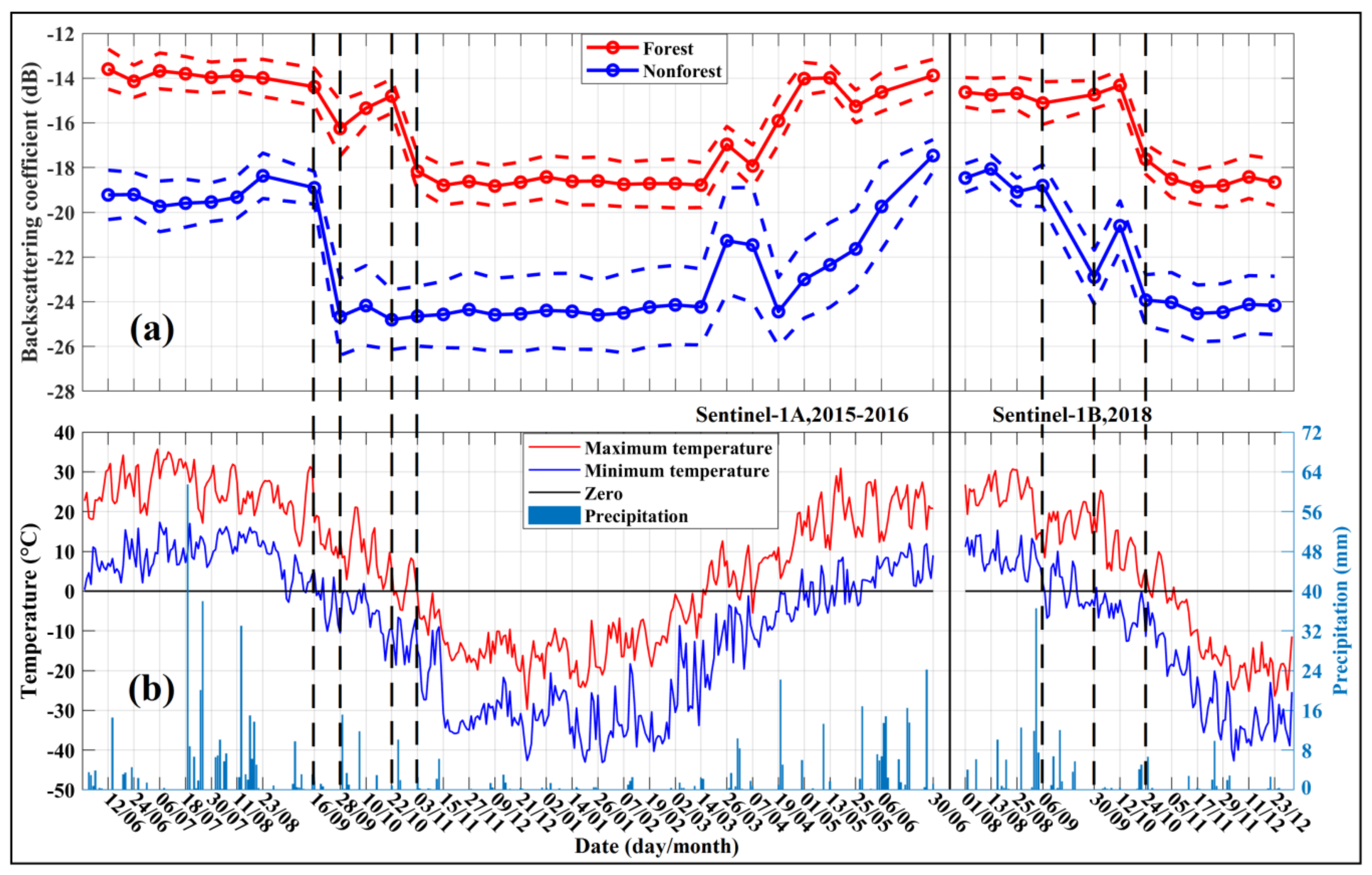
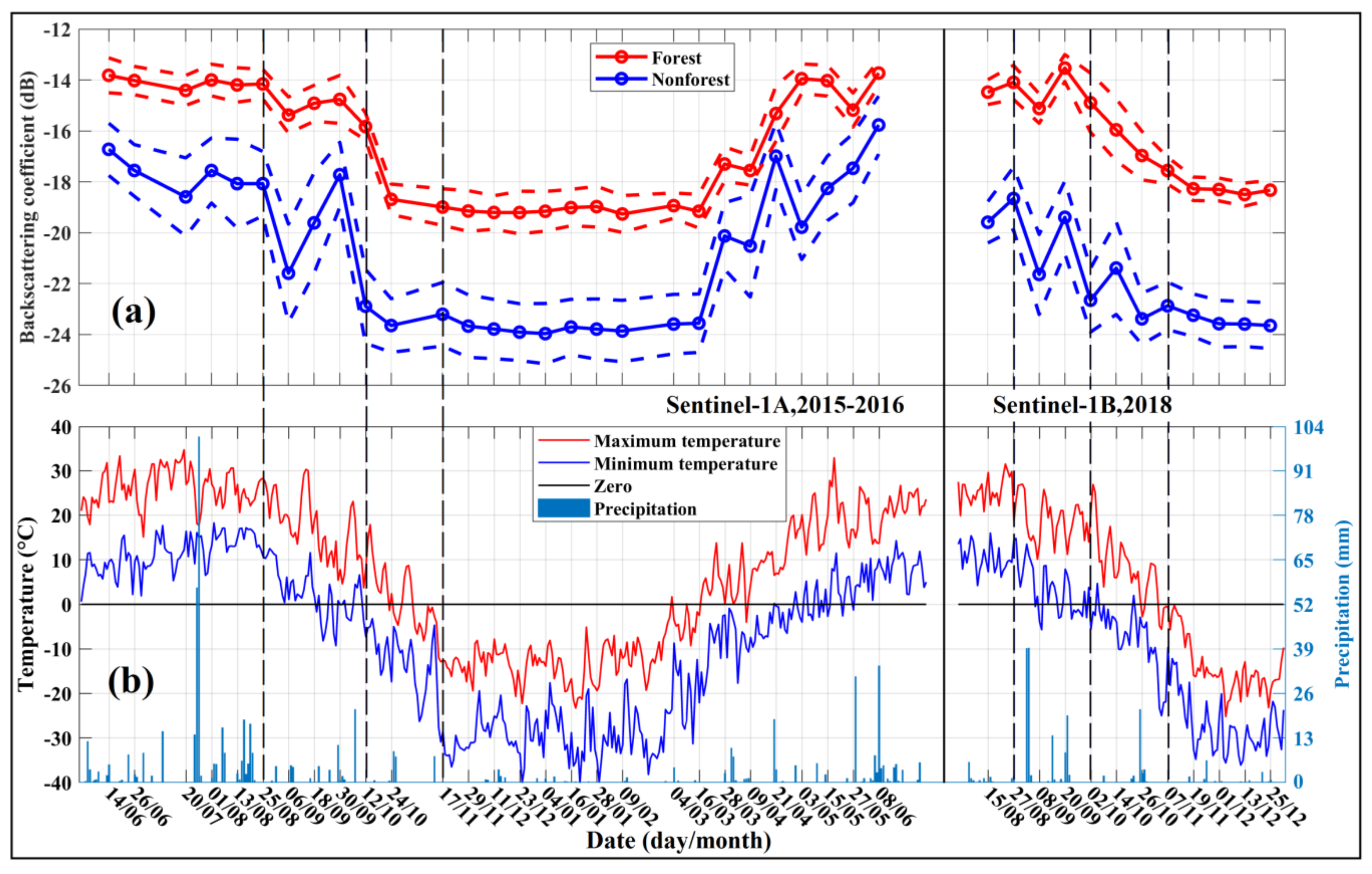
3. Temporal Behavior of Sentinel-1 Backscattering Coefficients over Forest and Non-Forest Plots

The temporal behavior of Sentinel-1 backscattering coefficients is explored using the typical forest and non-forest sampling plots defined in Section 2.3.1, i.e., type I with canopy cover >60% and type VII with canopy cover <10%. Figure 5a shows the mean values and standard deviations of VH Sentinel-1 backscattering time series using 20 plots of type I and 20 plots of type VII within the Strip-1-1. They are calculated in the linear scale, transformed into the dB scale, and drawn as red and blue lines in Figure 5a, respectively. As expected, the VH backscattering coefficients in forest plots are higher than those in non-forest plots due to the volume scattering within forest canopies. Lower backscattering coefficients are observed in the winter than those in the summer due to the decrease of volume scattering within canopies, snow coverage, and freezing effects.

The fluctuations of backscattering within summer or winter are small, while significant changes occur during the seasonal transitions between autumn and winter or between winter and spring, as shown in Figure 5a. For Sentinel-1A, a significant drop of approximately 6.0 dB appears between September 16th and 28th 2015 over non-forest plots. The drop of forest plots in the same period is only approximately 2.0 dB, which is much smaller than that of non-forest plots. Another drop of approximately 3.0 dB can be observed between October 22nd and November 3rd of 2015 over forest plots. The corresponding changes over non-forest plots in the same period are too weak to be observed. For Sentinel-1B, the largest drop of about 5.0 dB appears between September 6th and 30th 2018 over non-forest plots. No drop over forest plots in the same period can be observed. The largest drop of about 3.0 dB over forest plots occurs between September 30th and October 24th 2018. The drop over non-forest plots in the same period is only about 1.0 dB. It can be summarized that the date of the largest drop of backscattering over forest plots in the transition from autumn to winter is later than that of the largest drop of backscattering over non-forest plots.

Figure 5b shows daily maximum (i.e., red line) and minimum temperatures (i.e., blue line) and amount of precipitations (i.e., bars), which are reported by the Mohe weather station. An interesting phenomenon can be observed in which the two largest drops coincide with the critical temperatures. For the date of the largest drop of non-forest plots, the minimum temperature goes down across the freezing point. In 2015, the minimum temperatures in September 16th and 28th are higher and lower than 0 °C, respectively. In 2018, the minimum temperatures in September 6th and 30th are higher and lower than 0 °C, respectively. For the date of the largest drop over forest plots, the maximum temperature goes down across the freezing point. In 2015, the maximum temperatures in October 22nd and November 3rd are higher and lower than 0 °C, respectively. In 2018, the maximum temperatures in September 30th and October 24th are higher and lower than 0 °C, respectively.

The coincidence between the great changes of backscattering coefficients and the critical temperatures can also be observed in the transition from winter to spring. There is an increase of backscattering over both forest and non-forest plots when the maximum temperature firstly transits the freezing point between March 14th and 26th 2016. The increase, in terms of the mean value, over forest plots is about 2.0 dB, while that over non-forest plots is about 3.0 dB. The backscattering coefficients of both forest and non-forest plots also increase when the minimum temperature firstly approaches the freezing point between April 19th and May 1st 2016. However, it can be seen that the changes of backscattering coefficients during the transition from winter to spring are more complicated than those during the transition from autumn to winter, which may be attributed to the complicated status of ground thaw and snow melt.

Figure 6a shows statistics of the first group of sampling plots within the scene of Strip-3-1. Figure 6b shows the meteorological data provided by the Tahe weather station. The fluctuation of backscattering during the transition from autumn to winter is more complicated than that of Strip-1-1. In 2015, the backscattering coefficients of non-forest plots increase on September 18th and 30th because of the daily minimum temperatures wandering around 0 °C and the precipitations. The largest drop of backscattering over non-forest plots should be calculated using images acquired on August 25th and October 12th, while that over forest plots should be calculated using images acquired on October 12th and on or after November 17th. In 2018, the backscattering coefficients of non-forest plots increase twice on September 20th and October 14th, respectively. The largest drop of backscattering over non-forest plots should be calculated using images acquired on August 27th and October 2nd, while that over forest plots should be calculated using images acquired on October 2nd and on or after November 7th. Therefore, the new findings observed in Figure 5 can also be confirmed in Figure 6, although the variation is slightly complicated.

The latitudinal coverage of the Sentinel-1 data used in this study is about 46°–54°N and approximately 800 km in distance. The phenological effect has to be evaluated. Figure 7a shows the changes of the mean values of VH backscattering coefficients using the 200 sampling plots, i.e., 100 plots of type I, and 100 plots of type VII, collected in the west strip (i.e., Strip-1-1 to Strip-1-5). The lines with circles and triangles indicate the results from type I and type VII sampling plots, respectively. The statistical analyses are carried out in each scene of the west strip and are drawn in different colors. Figure 7b–f show the daily temperatures within scenes from Strip-1-1 to Strip-1-5, which were provided by the Mohe, Tulihe, Eerguna, Xinbaerkehuzuoqi and Aershan weather stations, respectively. As shown in Figure 7a, non-forest plots show larger variations among scenes than forest plots, which can be expected. The backscattering from non-forest plots is more sensitive to environmental factors, such as surface roughness, soil moisture, and snow coverage [20,35]. There is an abrupt increase of backscattering on October 10th of 2015 over non-forest fields of Strip-1-5. This can be attributed to the precipitation that occurred between October 9th and 10th of 2015.

Despite these differences among scenes, the largest drop over non-forest plots in these scenes occurs on the same date as the minimum temperature approaching or decreasing freezing points, while that over forest plots appears on the same date as the maximum temperature decreasing below freezing points. For 2015, the largest drop of backscattering coefficients over non-forest plots completes on approximately September 28th for all five scenes. The largest drop of backscattering coefficients of forest plots in the scene of Strip-1-1 occurs on November 3rd, which is about 12 days earlier than that of other scenes appears on November 15th. For 2018, the two critical dates are September 30th and November 5th. The largest drop of backscattering over non-forest plots can be observed between August 13th and September 30th, while that over forest plots can be obtained on September 30th and on or after November 5th.

The results shown in Figure 5, Figure 6 and Figure 7 are the statistical analysis only on the typical sampling plots with forest canopy coverage >60% (i.e., type I) and non-forest plots with canopy coverage <10% (i.e., type VII). Figure 8 shows the effects of forest canopy coverage on the temporal behavior of Sentinel-1 backscattering using the sampling plots of type I to type VII, as defined in Section 2.3.1. Lines in different colors represent the statistical mean backscattering of different types of sampling plots. An interesting phenomenon can be observed in the relationship between the magnitude of drops of backscattering coefficients and forest canopy coverage. On the date when the abrupt decrease of backscattering coefficients occurs over non-forest plots, i.e., September 28th, 2015 and September 30th, 2018, the decreased magnitude of backscattering coefficients is negatively correlated with forest canopy coverage. On the date when the abrupt decrease of backscattering coefficients occurs over forest plots, i.e., November 3rd, 2015 and October 24th, 2018, the decreased magnitude is positively correlated with forest canopy coverage.

Figure 5, Figure 6, Figure 7 and Figure 8 clearly present the temporal behaviors of Sentinel-1 images over forested and non-forested plots. The primary findings of this study are summarized as follows:

(1)

The date when the largest drop of backscattering coefficients over non-forest plots coincides with the date when the daily minimum temperature decreases across the freezing point; the decreased magnitude over non-forest plots is larger than that over forest plots.

(2)

The date when the largest drop of backscattering coefficients over forest plots coincides with the date when the daily maximum temperature decreases across the freezing point; the decreased magnitude over non-forest plots is smaller than that over forest plots.

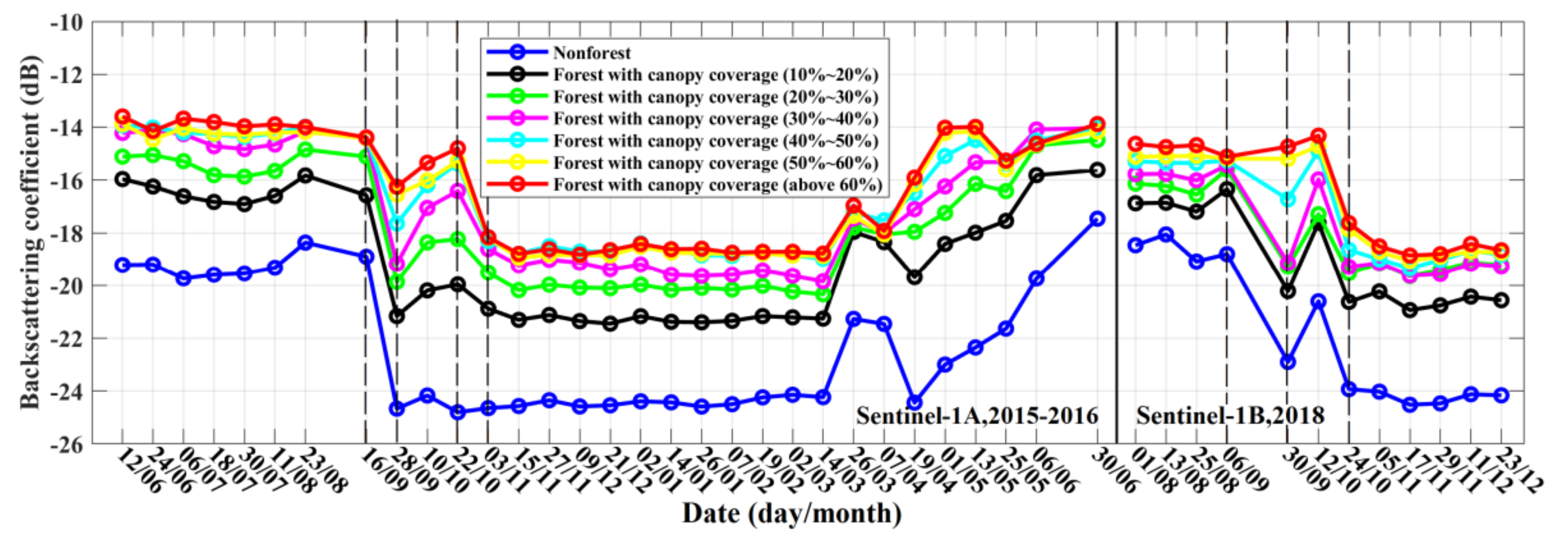
(3)

The decreased magnitude of backscattering coefficients when the daily minimum temperature decreases across the freezing point is negatively correlated with forest canopy coverage, while that when the daily maximum temperature decreases across the freezing point is positively correlated with forest canopy coverage.

4. Methods for Regional Forest Mapping

This study proposed two methods for the forest mapping based on the previously summarized new findings, i.e., the direct method for forest mapping and the indirect method for forest mapping via canopy coverage.

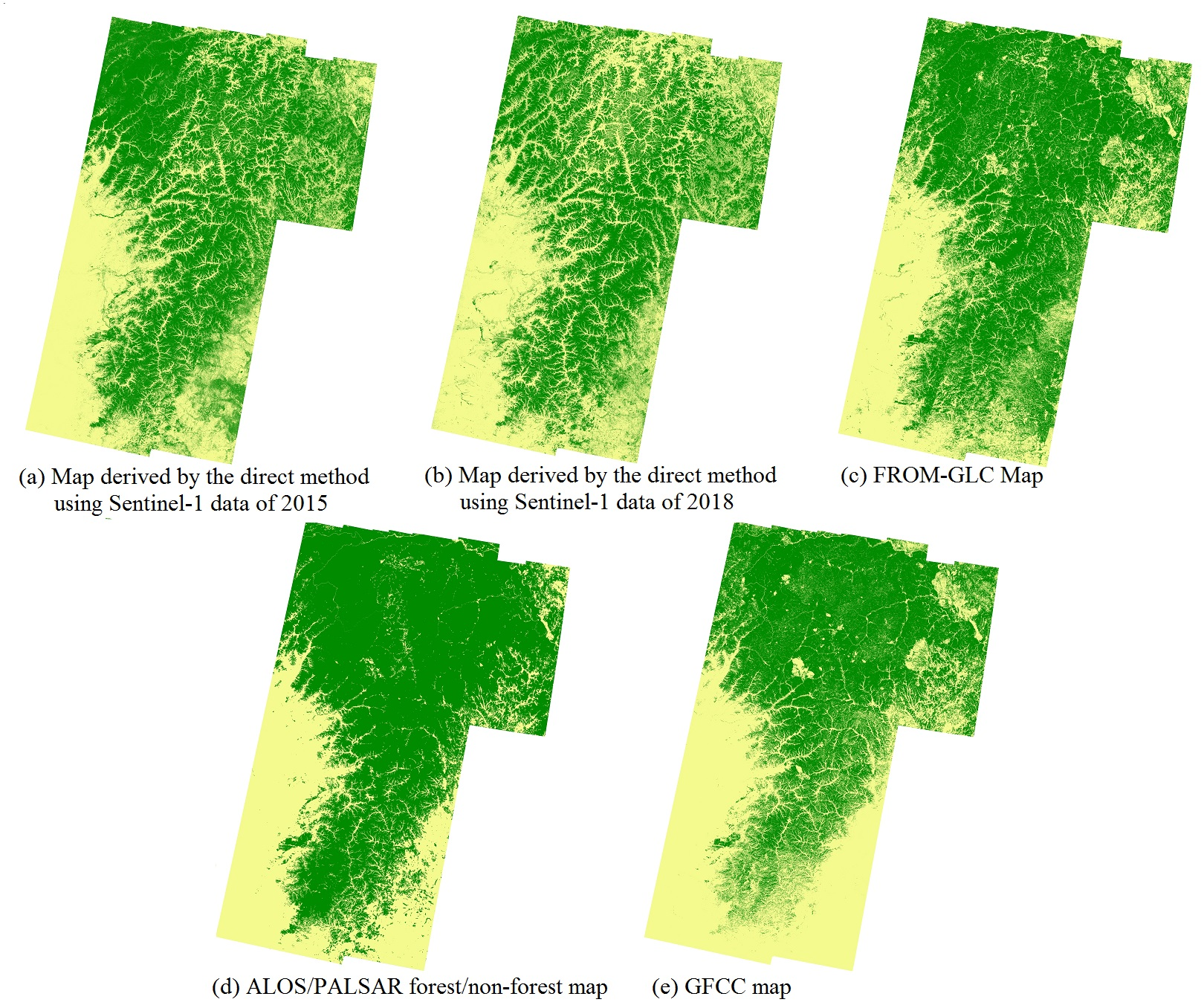
4.1. Direct Method for Forest Mapping

One new finding in last section is that the dates of the largest drops of backscattering coefficients over forest and non-forest plots are different. On the date when the largest drop of backscattering coefficients over non-forest plots occurs, the decreased magnitude of backscattering coefficients over forest plots is smaller than that over non-forest plots. On the date when the largest drop of backscattering coefficients over forest plots occurs, the decreased magnitude of backscattering coefficients over forest plots is larger than that over non-forest plots. Therefore, forest and non-forest plots can be directly distinguished by the relative size of the decreased magnitude of radar backscattering calculated from three dates of Sentinel-1 images. The direct method for forest/non-forest classification can be expressed as follows:

$$\left\{\begin{array}{c} forest pixels: {\sigma }_{Date1 }^0-{\sigma }_{Date2 }^0<{\sigma }_{Date2 }^0-{\sigma }_{Date3 }^0\\ non-forest pixels: {\sigma }_{Date1 }^0-{\sigma }_{Date2 }^0\ge {\sigma }_{Date2 }^0-{\sigma }_{Date3 }^0 \end{array}\right.$$

(3)

where ${\sigma }_{Date1 }^0$, ${\sigma }_{Date2 }^0$, and ${\sigma }_{Date3 }^0$ are backscattering coefficients in dB acquired on the date before the freezing date, i.e., the minimum temperature decreasing below 0 °C, on the date after the freezing date but before the maximum temperature decreasing below 0 °C, and on the date after the maximum temperature decreasing below 0 °C, respectively. In other words, there are two critical dates, i.e., one is when the daily minimum temperature decreases below 0 °C and the other is when daily maximum temperature decreases below 0 °C. Date1 should be before the first critical dates, Date3 should be on or after the second critical dates, and Date2 should be among the two critical dates.

4.2. Indirect Method for Forest Mapping via Canopy Coverage

The other new finding in the last section is summarized by the third point in Section 3. The decreased magnitudes of backscattering coefficients among Date1, Date2, and Date3 are correlated with forest canopy coverage. Therefore, forest canopy coverage can be estimated based on their correlations. Then, forest and non-forest pixels can be classified using the given threshold of forest canopy coverage. This method is referred to as the indirect method in this study. In the indirect method, the estimation model of forest canopy coverage is firstly developed through the statistical regression based on ${\sigma }_{Date1 }^0-{\sigma }_{Date2 }^0$ and ${\sigma }_{Date2 }^0-{\sigma }_{Date3 }^0$ using the sampling plots defined in Section 2.3.2. Three forest maps with a spatial resolution of 30 m × 30 m are further produced using the canopy coverage thresholds of 10%, 20%, and 30%, respectively.

4.3. Assessment of Forest Maps

The validation sampling plots defined in Section 2.3.3 are used as reference data to evaluate the accuracy of forest maps. Three indexes are used to describe the accuracy of maps in this study, including producer accuracy (PA), user accuracy (UA), and overall accuracy (OA). PA is the probability that a certain land cover of an area on the ground is classified as such, i.e., the ratio of correctly identified plots to the total number of predicted plots. UA is the probability that a value predicted to be in a certain class is actually in that class, i.e., the ratio of correctly identified plots to the total number of real plots. OA is the ratio of the number of correctly predicted items to the total number of real items.

Both the new maps produced in this study and the three maps prepared in Section 2.5 are evaluated by the same set of sampling plots. Therefore, the cross-comparison can be made between the new maps and publicly available maps.

5. Results

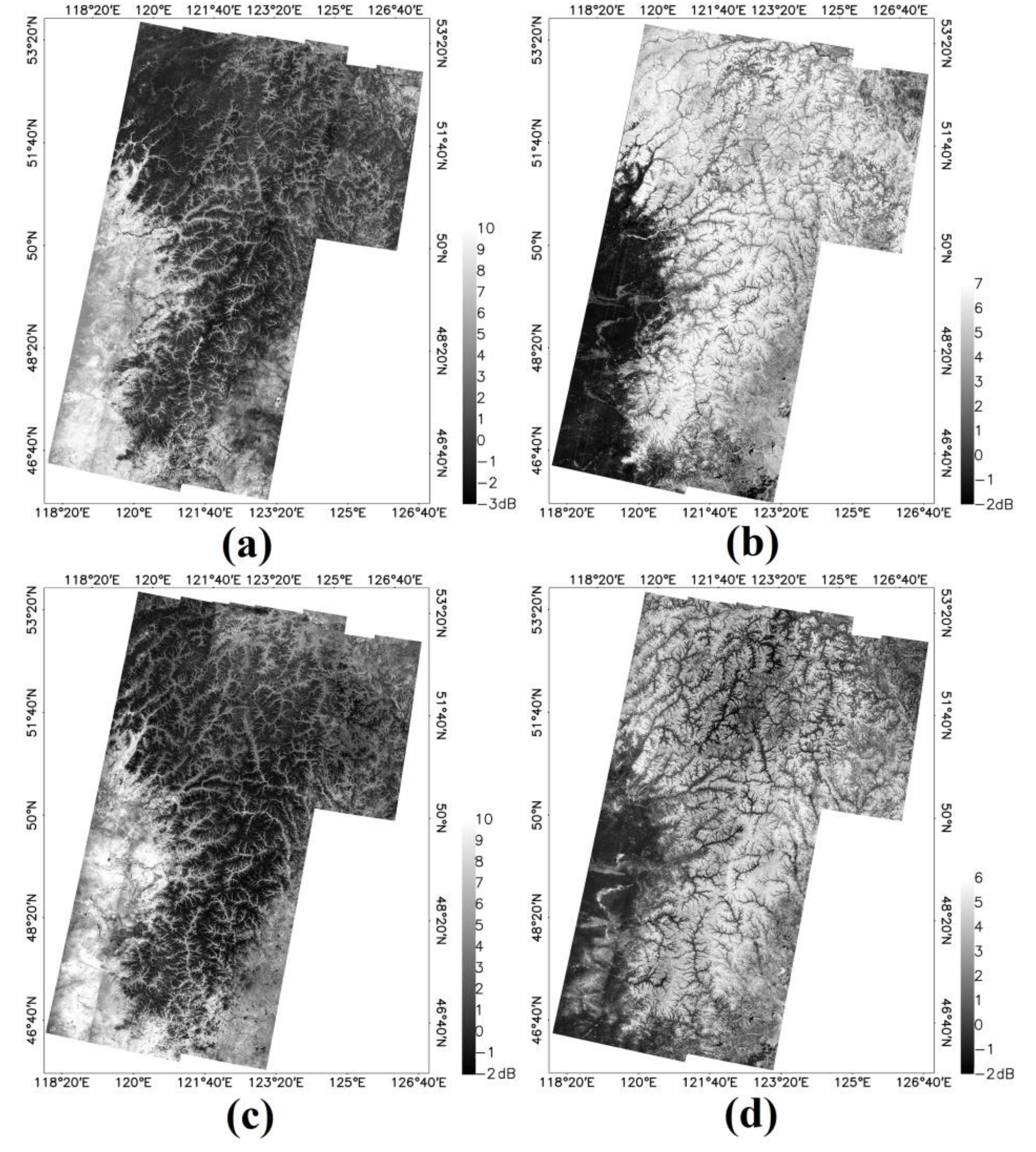
5.1. Intermediate Results of the Direct Method

Table 1. Acquisition dates of Sentinel-1 images used in regional forest mapping.

Year/Satellite	Scene	Date1	Date2	Date3
2015/Sentinel-1A	West Strip	August 23rd 2015	October 22nd 2015	November 15th 2015
	Middle Strip	July 25th 2015	October 5th 2015	November 10th 2015
	East Strip	August 25th 2015	October 12th 2015	November 17th 2015
2018/Sentinel-1B	West Strip	August 13th 2018	September 30th 2018	December 23rd 2018
	Middle Strip	September 1st 2018	October 19th 2018	December 18th 2018
	East Strip	August 27th 2018	October 2nd 2018	December 25th 2018

lists the acquisition dates of Sentinel-1 images used for the regional forest/non-forest mapping in this study. The Sentinel-1A images used as Date3 are all acquired within November, while those for Date2 are all within October. For Date1, the time interval is only two days between the west and the east strips, while the middle strip is approximately one month earlier due to the unavailability of Sentinel-1A images in August over the area. The Sentinel-1B images used as the Date3 are all acquired within December, which is after the second critical date, i.e., the daily maximum temperature decreasing below 0 °C. The Sentinel-1B images used as the Date2 are all acquired at the end of September or in the October, which are between the two critical dates. The Sentinel-1B images used as the Date1 are all acquired in August and just at the beginning of September, which are before the first critical date, i.e., the daily minimum temperature decreasing below 0 °C.

Figure 9 shows the mosaic of differences of Sentinel-1 images acquired on the dates listed in Table 1. Figure 9a,b is ${\sigma }_{Date1 }^0-{\sigma }_{Date2 }^0$ and ${\sigma }_{Date2 }^0-{\sigma }_{Date3 }^0$ using Sentinel-1A images acquired in 2015, respectively, while Figure 9c,d is ${\sigma }_{Date1 }^0-{\sigma }_{Date2 }^0$ and ${\sigma }_{Date2 }^0-{\sigma }_{Date3 }^0$ using Sentinel-1B images acquired in 2018, respectively. It can be seen from Figure 9a that forests have a smaller difference than non-forests compared with the maps in Figure 14c–e. Figure 9b appears to be converse of Figure 9a in that the forest shows larger difference than the non-forest. This phenomenon is further confirmed by Sentinel-1B images acquired in 2018, as shown in Figure 9c,d.

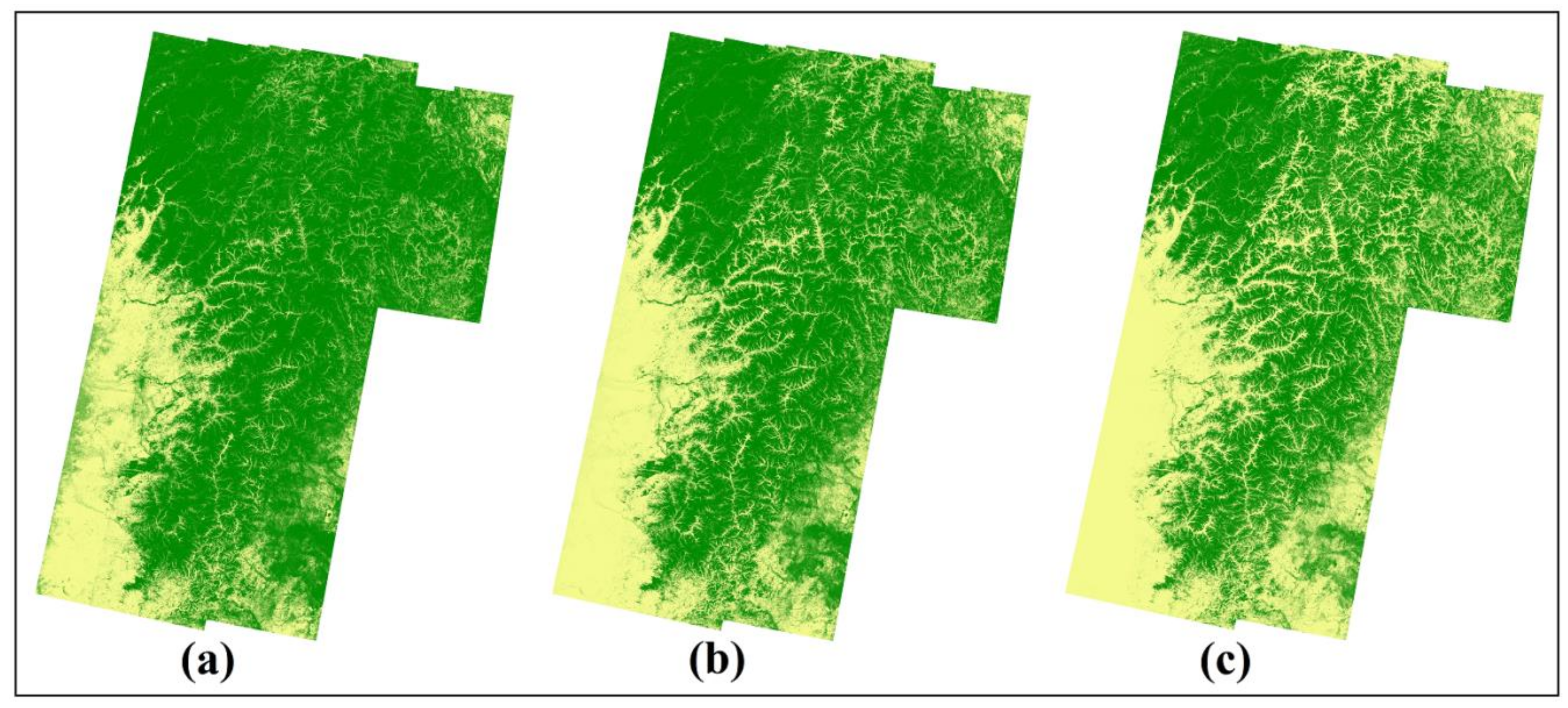
5.2. Intermediate Results of the Indirect Method

Table 2. Estimation models of forest canopy coverage used in the indirect method.

Model	Variable	Equation1	R2	RMSE
Model_2015	Combination	$\mathrm{C}=-4.37({\sigma }_{date1 }^0-{\sigma }_{date2 }^0$$)+2.18({\sigma }_{date2 }^0-{\sigma }_{date3 }^0)+36.83$	0.64	10.41%
Model_2018	Combination	$\mathrm{C}=-6.24({\sigma }_{date1 }^0-{\sigma }_{date2 }^0$$)+1.92({\sigma }_{date2 }^0-{\sigma }_{date3 }^0)+39.27$	0.53	12.03%

¹ C: canopy coverage (%).

lists the estimation models of forest canopy coverage developed in the indirect method, while Figure 10 shows the corresponding scatter plots of model estimations against canopy coverage based on HSRI of GoogleEarth^TM. Models developed based on the combination of ${\sigma }_{Date1 }^0-{\sigma }_{Date2 }^0$ and ${\sigma }_{Date2 }^0-{\sigma }_{Date3 }^0$ using Sentinel-1A images acquired in 2015 and Sentinel-1B images acquired in 2018 are named as model_2015 and model_2018, respectively. Table 2 confirms that the forest canopy coverage can indeed be estimated using either the Sentinel-1A images acquired in 2015 by the model_2015 or using Sentinel-1B images acquired in 2018 by the model_2018. The estimation error is approximately 10% and 12% in terms of root mean square error (RMSE) in model_2015 and model_2018, respectively.

Figure 11 shows the maps of forest canopy coverage produced by model_2015 and model_2018. Overall, their spatial patterns are similar. Some small differences between the two maps are exhibited, especially over the agricultural area and grassland in southeast and southwest parts. This is mainly introduced by the difference image of ${\sigma }_{Date1 }^0-{\sigma }_{Date2 }^0$, and it can be attributed to the different harvest times in 2015 and 2018.

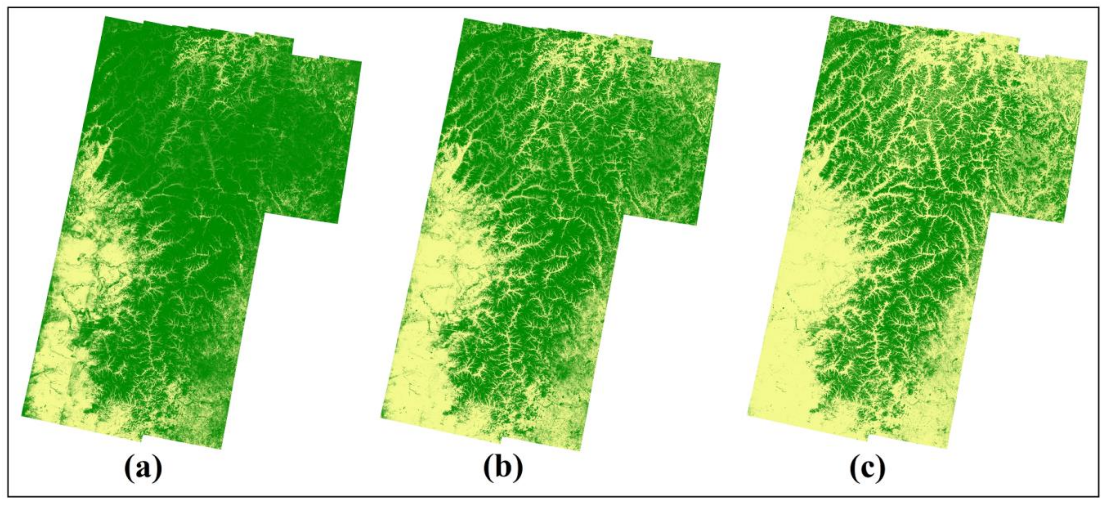
5.3. Assessments of Forest Maps

Figure 12 and Figure 13 show the forest maps produced by the indirect method using model_2015 and model_2018, respectively. The three maps in each figure are generated using canopy coverage thresholds of 10%, 20%, and 30%, respectively. It can be seen in each figure that the area of classified forest decreases as the increasing of canopy coverage thresholds. Figure 14 shows the forest maps produced by the direct method using Sentinel-1 data of 2015 and 2018 and released maps prepared in Section 2.5. The spatial pattern of these maps is similar, although their details are different more or less. It can be seen that Figure 14a,b are more similar to the maps of b,c in Figure 12 and Figure 13, respectively, which can be explained by Figure 8. According to Figure 8, the direct method is more appropriate for forest areas with adequate canopy coverage (higher than approximately 20%), while the maps in b,c in Figure 12 and Figure 13 are derived using canopy coverage thresholds of 20% and 30%, respectively.

Table 3. Assessment of forest/non-forest maps (484 sampling plots are collected, including 289 forest and 195 non-forest samples plots). OA: overall accuracy, PA: producer accuracy, UA: user accuracy.

Maps		F1	N2	Total	PA (%)	Maps		F	N	Total	PA (%)
model_2015 >10%	F	288	37	325	88.62	Direct method using data of 2015	F	261	3	264	98.86
	N	1	158	159	99.37		N	28	192	220	87.27
	UA (%)	99.65	81.03	/	OA: 92.15		UA (%)	90.31	98.46	/	OA: 93.60
model_2015 >20%	F	280	21	299	93.65	Direct method using data of 2018	F	248	16	264	93.94
	N	9	174	185	94.05		N	41	179	220	81.36
	UA (%)	96.89	89.23	/	OA: 93.80		UA (%)	85.81	91.79	/	OA: 88.22
model_2015 >30%	F	257	5	262	98.09	FROM-GLC	F	275	28	303	90.76
	N	32	190	222	85.59		N	14	167	181	92.27
	UA (%)	88.93	97.44	/	OA: 92.36		UA (%)	95.16	85.64	/	OA: 91.32
model_2018 >10%	F	287	46	333	86.19	ALOS/PALSAR	F	283	21	304	93.09
	N	2	149	151	98.68		N	6	174	180	96.67
	UA (%)	99.31	76.41	/	OA: 90.08		UA (%)	97.92	89.23	-	OA: 94.42
model_2018 >20%	F	270	17	287	94.08	GFCC	F	263	3	266	98.87
	N	19	178	197	90.36		N	26	192	218	88.07
	UA (%)	93.43	91.28	/	OA: 92.56		UA (%)	91.00	98.46	/	OA: 94.01%
model_2018 >30%	F	231	2	233	99.14
	N	58	193	251	76.89
	UA (%)	79.93	98.97	/	OA: 87.60

¹ F: forest; ² N: non-forest.

reports the confusion matrix of all forest maps assessed using the validation sampling plots defined in Section 2.3.3. For the indirect method, the overall accuracy firstly increases and then decreases as the increasing of canopy coverage threshold in each model. The map with a canopy coverage threshold of 20% has the best accuracy for the two models. For model_2018 used in the indirect method, the overall accuracies of the three maps with different canopy coverage thresholds are 90.08%, 92.56%, and 87.60%, respectively. The accuracies of the three maps produced by model_2015 are better than their corresponding maps by model_2018. The overall accuracies of the three maps are 92.15%, 93.80%, and 92.36%, respectively.

The overall accuracy of the forest map produced by the direct method using Sentinel-1A images acquired in 2015 is 93.60%, which is better than the map produced by the direct method using Sentinel-1 images acquired in 2018 (i.e., 88.22%) and the best map of model_2018 (i.e., 92.56%), while it is approximately the same with the best map of model_2015 (i.e., 93.80%). However, they have different rates of misclassification. In the map of model_2015 with a canopy coverage threshold of 20%, 21 non-forest plots are misclassified as forest plots, while 9 forest plots are misclassified as non-forest plots. In the map of the direct method using Sentinel-1 data of 2015, 3 non-forest plots are misclassified as forest plots, and 28 forest plots are misclassified as non-forest plots. In terms of UA and PA, the map of the direct method using Sentinel-1 data of 2015 is closest to the map of model_2015 with a canopy coverage threshold of 30%. This coincides with the map of the direct method using Sentinel-1 data of 2018 and the map of model_2018 with a canopy coverage threshold of 30%. In other words, the direct method is good at distinguishing non-forest plots of bareground and forest plots with sufficient canopy coverage, while it demonstrates poor performance on identifying sparse forest with canopy coverage smaller than 30%.

The overall accuracy of forest maps derived from released land cover maps are 94.42%, 94.01%, and 91.32%, corresponding to ALOS/PALSAR, GFCC, and FROM-GLC, respectively. It can be seen that the overall accuracy of the best map of model_2018 is slightly higher than that of FROM-GLC, while the best map of model_2015 or that of the direct method using Sentinel-1 data of 2015 is approximately the same as GFCC.

6. Discussion

6.1. Specific Features of C-Band Backscattering during the Transition from Autumn to Winter

The seasonal behavior of C-band SAR backscattering over forested area is not a new topic. Many papers on this topic were published in the 1990s [36,37,38]. The decrease of radar backscattering from thaw in summer to frozen in winter has been well documented based on the observation of ERS-1/2 SAR images. Unlike these early studies that reported the difference of SAR backscattering between summer and winter, this study revealed the specific features of C-band backscattering during the transition from autumn to winter. We found that the dates of the largest drop of SAR backscattering over forest and non-forest plots were different. Furthermore, the new finding could be used to conduct forest/non-forest mapping. The accuracy of forest/non-forest maps produced based on the new finding was as high as that of well-known maps. The successful capture of these new findings should be attributed to the 12-day revisit capability of Sentinel-1A or Sentinel-1B, which is much shorter than that of ERS SAR, i.e., 35 days.

6.2. Significance of Date2 for Forest Mapping Using Sentinel-1 Images

This study investigated the temporal behaviors of Sentinel-1 backscattering of VH polarization over typical forest and non-forest plots. Two critical dates were identified for the forest mapping, i.e., the first date is when the minimum temperature decreased below 0 °C, and the second date is when the maximum temperature decreased below 0 °C. Then, the direct and indirect methods were proposed for the forest mapping using only images of 3 dates, i.e., Date1, Date2 and Date3, as shown in Table 1. Date1 can be any date in summer before the first date so long as it is not affected by precipitations. Date3 can be any date in winter after the second date so long as the maximum temperature decreased below 0 °C. However, Date2 must be between the first and second dates. The time window for Date2 is much narrower than those of Date1 and Date3, which is only approximately one month in the test site of this study. It can be anticipated that the time window for Date2 should be narrowed or even disappear as the latitude decreases. The availability of images on Date2 determines the applicability of the proposed forest mapping methods.

6.3. Further Exploration for Physical Understanding of the New Findings

Based on the observation of 450 scenes of C-band SAR images acquired by Sentinel-1A and Sentinel-1B over an area of 318,898.62 km² in this study, we found that the dates of the largest drops of backscattering coefficients over forest and non-forest plots were different during the transition from autumn to winter. We interpreted this phenomenon based on daily temperatures and further found that the largest drop of non-forest plots occurred around the date of the minimum temperature decreasing below 0 °C, while that of forest plots occurred around the date of the maximum temperature decreasing below 0 °C. However, it has to be kept in mind that the SAR backscattering is directly determined by the status of moisture but not the temperature. Temperature is only a factor that is highly related to the status of freeze or thaw of moisture. According to our observations and understandings, the interpretation is that during the days when the maximum temperature is above 0 °C and the minimum temperature is below 0 °C, the snow/frost/ice on canopies is easier to be melted away than that on the ground surfaces. Therefore, the backscattering of non-forest plots decrease earlier than that of forest plots. The backscattering of both types of plots decrease in deep winter when the maximum temperature is below 0 °C, because the snow/frost/ice both on canopies and the ground surface no longer melts away.

The forest phenology also affects the received SAR signal. The VH polarization is highly influenced by volume scattering, which is dependent on the forest structure and the status of water contents. The status of water content or vegetation phenology are both correlated with temperatures. Therefore, the temporal behavior of Sentinel-1 backscattering is interpreted using daily temperatures and precipitations in this study. More field observations and experiments should be carried out in the future in order to confirm this interpretation or reach a thorough understanding of the observed phenomena.

6.4. Terrain Effects

The terrain effect is an important issue that should be specifically considered in the application of SAR images, especially over mountainous areas. In this study, we firstly investigated the seasonal behavior of SAR backscattering and then produced forest maps using the proposed methods. For the quantitative analysis of seasonal behavior over sampling plots collected on different terrain slopes, terrain effects on the backscattering coefficients have to be corrected as performed in Section 2.2. Otherwise, the seasonal behavior would be heavily disturbed or even buried by terrain effects. Generally, the land cover should be considered in the terrain corrections. However, in this study, it is not proper to use other source of land cover data in the terrain corrections because one objective of this study is forest mapping. Figure 3 shows that the dependence of backscatter on the local incidence angle was successfully corrected. Therefore, we believe that the terrain correction carried out in this study is sufficient for the following analysis, although the method we used is not the most updated one, and the land cover was not considered.

For the forest mapping using the proposed methods in this study, the situation is different from the quantitative analysis of seasonal behavior over sampling plots. Both direct and indirect methods are developed based on the difference of SAR images on the dB scale. Mathematically, the image difference on dB equals the image ratio on a linear scale (backscattering coefficients range between 0 and 1). It has been demonstrated that the terrain effects on backscattering coefficients can be reduced by image ratios so long as the two images are accurately co-registered and acquired with similar incident angles [39,40]. From this point, the correction of terrain effects on backscattering coefficients can be avoided in the forest mapping using the proposed method in this study.

6.5. Latitude and Precipitation Effects

The two critical dates identified in this study are determined by the minimum and the maximum temperatures. Unavoidably, they may be affected by latitudes and also by altitudes over higher mountains. The latitude span in this study is about 8°. A slight effect caused by latitude has been observed on the west strip on November 3rd and November 15th, 2015 in Figure 7. It should be considered in the selection of Sentinel-1 images.

It is well known that the SAR backscattering is easily affected by precipitations because microwaves are sensitive to the water content. The precipitation effects, including rainfall and snowfall, have been observed in Section 3. The indirect and direct methods proposed in this study provide users with a large flexibility in the selection of Date1 and Date3 Sentinel-1 images to avoid effects of precipitations.

7. Conclusions

The seasonal behavior of C-band SAR backscattering of VH polarization on typical forest and non-forest plots was systemically investigated based on 450 scenes of Sentinel-1 images over an area of 318,898.62 km². Interesting temporal features have been observed in this study. Based on the observed critical temporal features, the indirect and direct methods have been proposed in this study for forest mapping. Results showed that the regional forest maps produced by both the direct method and the indirect method using three images have accuracies of approximately 93%, which are comparable to that of forest maps derived from released land cover maps. The latitude and precipitation effects in the data selection and the terrain effects in the image processing have to be considered. This study proposed new methods for the regional forest mapping using C-band SAR images. The applicability of the proposed methods over larger areas will be further examined in future studies.

References

1. Stenger, A.; Harou, P.; Navrud, S. Valuing Environmental Goods and Services Derived from the Forests. J. For. Econ. 2010, 15, 1–14. [Google Scholar] [CrossRef]
2. Martone, M.; Rizzoli, P.; Wecklich, C.; Gonzalez, C.; Bueso-Bello, J.L.; Valdo, P.; Schulze, D.; Zink, M.; Krieger, G.; Moreira, A. The global forest/non-forest map from TanDEM-X interferometric SAR data. Remote Sens. Environ. 2018, 205, 352–373. [Google Scholar] [CrossRef]
3. Le Toan, T.; Quegan, S.; Davidson, M.; Balzter, H.; Paillou, P.; Papathanassiou, K.; Plummer, S.; Rocca, F.; Saatchi, S.; Shugart, H. The BIOMASS mission: Mapping global forest biomass to better understand the terrestrial carbon cycle. Remote Sens. Environ. 2011, 115, 2850–2860. [Google Scholar] [CrossRef] [Green Version]
4. Bartholome, E.; Belward, A.S. GLC2000: A new approach to global land cover mapping from Earth observation data. Int. J. Remote Sens. 2005, 26, 1959–1977. [Google Scholar] [CrossRef]
5. Bontemps, S.; Defourny, P.; Bogaert, E.V.; Arino, O.; Kalogirou, V.; Perez, J.R. GlobCover 2009—Product Description Manual; ESA: Paris, France, 2011. [Google Scholar]
6. Chen, J.; Chen, J.; Liao, A.; Cao, X.; Chen, L.; Chen, X.; He, C.; Han, G.; Peng, S.; Lu, M. Global land cover mapping at 30 m resolution: A POK-based operational approach. ISPRS J. Photogramm. Remote. Sens. 2015, 103, 7–27. [Google Scholar] [CrossRef] [Green Version]
7. Gong, P.; Wang, J.; Yu, L.; Zhao, Y.; Zhao, Y.; Liang, L.; Niu, Z.; Huang, X.; Fu, H.; Liu, S. Finer resolution observation and monitoring of global land cover: First mapping results with Landsat TM and ETM+ data. Int. J. Remote Sens. 2013, 34, 2607–2654. [Google Scholar] [CrossRef] [Green Version]
8. Hansen, M.C.; Potapov, P.V.; Moore, R.; Hancher, M.; Turubanova, S.A.; Tyukavina, A.; Thau, D.; Stehman, S.V.; Goetz, S.J.; Loveland, T.R. High-resolution global maps of 21st-century forest cover change. Science 2014, 342, 850–853. [Google Scholar] [CrossRef] [Green Version]
9. Rüetschi, M.; Schaepman, M.E.; Small, D. Using Multitemporal Sentinel-1 C-band Backscatter to Monitor Phenology and Classify Deciduous and Coniferous Forests in Northern Switzerland. Remote. Sens. 2017, 10. [Google Scholar]
10. Mohammadimanesh, F.; Salehi, B.; Mahdianpari, M.; Brisco, B.; Motagh, M. Multi-temporal, multi-frequency, and multi-polarization coherence and SAR backscatter analysis of wetlands. ISPRS J. Photogramm. Remote. Sens. 2018, 142, 78–93. [Google Scholar] [CrossRef]
11. Quegan, S.; Rhodes, I. Statistical-Models for Polarimetric Data - Consequences, Testing and Validity. Int. J. Remote Sens. 1995, 16, 1183–1210. [Google Scholar] [CrossRef]
12. Kimes, D.S.; Ranson, K.J.; Sun, G. Inversion of a forest backscatter model using neural networks. Int. J. Remote Sens. 1997, 18, 2181–2199. [Google Scholar] [CrossRef]
13. Askne, J.I.H.; Dammert, P.B.G.; Ulander, L.M.H.; Smith, G. C-band repeat-pass interferometric SAR observations of the forest. IEEE Trans. Geosci. Remote Sens. 1997, 35, 25–35. [Google Scholar] [CrossRef]
14. Chen, K.S.; Huang, W.P.; Tsay, D.H.; Amar, F. Classification of multifrequency polarimetric SAR imagery using a dynamic learning neural network. IEEE Trans. Geosci. Remote Sens. 1996, 34, 814–820. [Google Scholar] [CrossRef]
15. Hoekman, D.H.; Quinones, M.J. Land cover type and biomass classification using AirSAR data for evaluation of monitoring scenarios in the Colombian Amazon. In Proceedings of the 2nd International Workshop on Retrieval of Bio- and Geophysical parameters from SAR data for land applications, Noordwijk, The Netherlands, 21–23 October 1998; pp. 215–223. [Google Scholar]
16. Ranson, K.J.; Sun, G.Q. An evaluation of AIRSAR and SIR-C/X-SAR images for mapping northern forest attributes in Maine, USA. Remote Sens. Environ. 1997, 59, 203–222. [Google Scholar] [CrossRef]
17. Degrandi, G.F.; Lemoine, G.G.; Degroof, H.; Lavalle, C.; Sieber, A.J. Fully Polarimetric Classification of the Black-Forest Maestro-1 Airsar Data. Int. J. Remote Sens. 1994, 15, 2755–2775. [Google Scholar] [CrossRef]
18. Townsend, P.A. Mapping seasonal flooding in forested wetlands using multi-temporal radarsat SAR. Photogramm. Eng. Remote Sens. 2001, 67, 857–864. [Google Scholar]
19. Conway, J. Evaluating ERS-1 SAR data for the discrimination of tropical forest from other tropical vegetation types in Papua New Guinea. Int. J. Remote Sens. 1997, 18, 2967–2984. [Google Scholar] [CrossRef]
20. Quegan, S.; Le Toan, T.; Yu, J.J.; Ribbes, F.; Floury, N. Multitemporal ERS SAR analysis applied to forest mapping. IEEE Trans. Geosci. Remote Sens. 2000, 38, 741–753. [Google Scholar] [CrossRef]
21. Proisy, C.; Mougin, E.; Dufrêne, E.; Dantec, V.L. Monitoring seasonal changes of a mixed temperate forest using ERS SAR observations. IEEE Trans. Geosci. Remote Sens. 2000, 38, 540–552. [Google Scholar] [CrossRef]
22. Ulaby, F.T.; Moore, R.K.; Fung, A.K.; Rasool, S.I. Book-Review—Microwave Remote Sensing—Active and Passive. Space. Sci. Rev. 1983, 35, 295. [Google Scholar]
23. Pulliainen, J.T.; Mikkela, P.J.; Hallikainen, M.T.; Ikonen, J.P. Seasonal dynamics of C-band backscatter of boreal forests with applications to biomass and soil moisture estimation. IEEE Trans. Geosci. Remote Sens. 1996, 34, 758–770. [Google Scholar] [CrossRef]
24. Balzter, H. Forest mapping and monitoring with interferometric synthetic aperture radar (InSAR). Prog. Phys. Geogr. 2001, 25, 159–177. [Google Scholar] [CrossRef] [Green Version]
25. Song, Y.; Wang, J. Mapping Winter Wheat Planting Area and Monitoring Its Phenology Using Sentinel-1 Backscatter Time Series. Remote Sens. 2019, 11. [Google Scholar] [CrossRef] [Green Version]
26. Nasrallah, A.; Baghdadi, N.; El Hajj, M.; Darwish, T.; Belhouchette, H.; Faour, G.; Darwich, S.; Mhawej, M. Sentinel-1 Data for Winter Wheat Phenology Monitoring and Mapping. Remote Sens. 2019, 11, 2228. [Google Scholar] [CrossRef] [Green Version]
27. Huang, W.; Hu, Y.; Chang, Y.; Liu, M.; Li, Y.; Ren, B.; Shi, S. Effects of Fire Severity and Topography on Soil Black Carbon Accumulation in Boreal Forest of Northeast China. Forests 2018, 9, 408. [Google Scholar] [CrossRef] [Green Version]
28. Attema, E.; Bargellini, P.; Edwards, P.; Levrini, G.; Lokas, S.; Moeller, L.; Rosichtell, B.; Secchi, P.; Torres, R.; Davidson, M. Sentinel-1-the radar mission for GMES operational land and sea services. Esa Bull. 2007, 131, 10–17. [Google Scholar]
29. Nagler, T.; Rott, H.; Hetzenecker, M.; Wuite, J.; Potin, P. The Sentinel-1 Mission&58; New Opportunities for Ice Sheet Observations. Remote Sens. 2015, 7, 9371. [Google Scholar]
30. Sun, G.; Ranson, K.J.; Kharuk, V.I. Radiometric slope correction for forest biomass estimation from SAR data in the Western Sayani Mountains, Siberia. Remote Sens. Environ. 2002, 79, 279–287. [Google Scholar] [CrossRef]
31. Ohtsu, N. A Threshold Selection Method from Gray-Level Histograms. IEEE Trans. Syst. Man. Cybern. 2007, 9, 62–66. [Google Scholar] [CrossRef] [Green Version]
32. Rose, S. Forests and Climate Change Working Paper 10. Tech. Rep. 2012, 11, 269–272. [Google Scholar]
33. Shimada, M.; Itoh, T.; Motooka, T.; Watanabe, M.; Thapa, R. Generation of the first PALSAR-2 global mosaic 2014/2015 and change detection between 2007 and 2015 using the PALSAR and PALSAR-2. In Proceedings of the Geoscience and Remote Sensing Symposium, Beijing, China, 10–15 July 2016; pp. 3871–3872. [Google Scholar]
34. Shimada, M.; Itoh, T.; Motooka, T.; Watanabe, M.; Shiraishi, T.; Thapa, R.; Lucas, R. New global forest/non-forest maps from ALOS PALSAR data (2007–2010). Remote Sens. Environ. 2014, 155, 13–31. [Google Scholar] [CrossRef]
35. Ulaby, F.T.; Moore, R.K.; Fung, A.K. Microwave Remote Sensing: Active and Passive v.2: Radar Remote Sensing and Surface Scattering and Emission Theory; Addison-Wesley Pub. Co: Boston, MA, USA, 1982. [Google Scholar]
36. Rignot, E.J.M.; Williams, C.L.; Way, J.B.; Viereck, L.A. Mapping of Forest Types in Alaskan Boreal Forests Using Sar Imagery. IEEE Trans. Geosci. Remote Sens. 1994, 32, 1051–1059. [Google Scholar] [CrossRef] [Green Version]
37. Way, J.; Rignot, E.J.M.; Mcdonald, K.C.; Oren, R.; Kwok, R.; Bonan, G.; Dobson, M.C.; Viereck, L.A.; Roth, J.E. Evaluating the Type and State of Alaska Taiga Forests with Imaging Radar for Use in Ecosystem Models. IEEE Trans. Geosci. Remote Sens. 1994, 32, 353–370. [Google Scholar] [CrossRef]
38. Wang, Y.; Kasischke, E.S.; Melack, J.M.; Davis, F.W.; Christensen, N.L. The Effects of Changes in Loblolly-Pine Biomass and Soil-Moisture on Ers-1 Sar Backscatter. Remote Sens. Environ. 1994, 49, 25–31. [Google Scholar] [CrossRef]
39. Ranson, K.J.; Saatchi, S.; Sun, G.Q. Boreal forest ecosystem characterization with SIR-C/XSAR. IEEE Trans. Geosci. Remote Sens. 1995, 33, 867–876. [Google Scholar] [CrossRef]
40. Belenguer-Plomer, M.A.; Tanase, M.A.; Fernandez-Carrillo, A.; Chuvieco, E. Burned area detection and mapping using Sentinel-1 backscatter coefficient and thermal anomalies. Remote Sens. Environ. 2019, 233. [Google Scholar] [CrossRef]
Figure 1. The location and terrain conditions of the study area: (a) Location of the Greater Khingan Mountains in China; (b) Digital elevation map (DEM) of study areas from Shuttle Radar Topography Mission (SRTM) data; (c) Histogram of the terrain slope; (d) Spatial coverage of Sentinel-1 data on a true color image from GoogleEarthTM and the distribution of 6 weather stations (represented by green dots) used in this study. The blue, orange, and purple polygons are locations of the west, middle, and east strips of Sentinel-1 images, respectively.
Remotesensing 12 01485 g001
Figure 2. Temporal distributions of the Sentinel-1 images acquisition (month/year).
Remotesensing 12 01485 g002
Figure 3. Correction of terrain effects using Equation (1) on images of Strip-1-1 acquired on June 12 2015: (a,b) are the images of cross-polarimetric (i.e., VH) processed by the Sentinel Application Platform (SNAP) and further corrected using Equation (1), respectively; (c,d) are enlarged images of (a,b) over the area covered by the black box, respectively; (e) is the scatter plot of the backscattering coefficient against the local incidence angle before and after the correction of Equation (1).
Remotesensing 12 01485 g003
Figure 4. Spatial distributions of sampling plots used in this study. The background is Google EarthTM image with black polygons indicating the spatial coverage of Sentinel-1 images. The squares, circles, and triangles with different colors indicate different types of sampling plots.
Remotesensing 12 01485 g004
Figure 5. Time series of VH backscattering coefficients on the type I and type VII sampling plots of the first group and corresponding daily temperatures and amount of precipitations within the scene of Strip-1-1: (a) Backscattering coefficients of forest plots (in red) and non-forest plots (in blue), solid lines are the mean values and dotted lines are standard deviations; (b) Daily temperatures and amount of precipitations.
Remotesensing 12 01485 g005
Figure 6. Time series of VH backscattering coefficients on the type I and type VII sampling plots of the first group and corresponding daily temperatures and amount of precipitations within the scene of Strip-3-1: (a) Backscattering coefficients of forest plots (in red) and non-forest plots (in blue), solid lines are the mean values and dotted lines are standard deviations; (b) Daily temperatures and amount of precipitations.
Remotesensing 12 01485 g006
Figure 7. Time series of VH backscattering coefficients on the type I and type VII sampling plots of the first group and corresponding daily temperatures and amount of precipitation within scenes from Strip-1-1 to Strip-1-5: (a) Backscattering coefficients of forest plots (in red) and non-forest plots (in blue); (bf) are daily temperatures and amount of precipitations within scenes from Strip-1-1 to Strip-1-5, respectively.
Remotesensing 12 01485 g007
Figure 8. Effects of forest canopy coverage on the temporal behavior of backscattering using Sentinel-1 data. Lines in different colors indicate the statistical mean backscattering of statistics on different types of sampling plots.
Remotesensing 12 01485 g008
Figure 9. Differences of Sentinel-1 images listed in Table 1: (a) σ D a t e 1   0 σ D a t e 2   0 using Sentinel-1A in 2015; (b) σ D a t e 2     0 σ D a t e 3   0 using Sentinel-1A in 2015; (c) σ D a t e 1   0 σ D a t e 2   0 using Sentinel-1B in 2018; (d) σ D a t e 2     0 σ D a t e 3   0 using Sentinel-1B in 2018.
Remotesensing 12 01485 g009
Figure 10. Validation of estimation models of forest canopy coverage: (a) model_2015 and (b) model_2018.
Remotesensing 12 01485 g010
Figure 11. Maps of forest canopy coverage produced by different indirect estimation models: (a) model_2015 and (b) model_2018.
Remotesensing 12 01485 g011
Figure 12. Forest maps produced by different thresholds of canopy coverage estimated by the model_2015: (a) >10%; (b) >20%; (c) >30%. Green: forest, Yellow: non-forest.
Remotesensing 12 01485 g012
Figure 13. Forest maps produced by different thresholds of canopy coverage estimated by the model_2018: (a) >10%; (b) >20%; (c) >30%. Green: forest, Yellow: non-forest.
Remotesensing 12 01485 g013
Figure 14. Forest maps: (a) The map derived by the direct method using Sentinel-1 data of 2015; (b) The map derived by the direct method using Sentinel-1 data of 2018; (c) Finer Resolution Observation and Monitoring of Global Land Cover (FROM-GLC); (d) ALOS/PALSAR forest/non-forest; (e) Landsat Global Forest Cover Change (GFCC) dataset. Green: forest, Yellow: non-forest.
Remotesensing 12 01485 g014