Ash Presence and Abundance Derived from Composite Landsat and Sentinel-2 Time Series and Lidar Surface Models in Minnesota, USA


 ,
,
Abstract
1. Introduction
2. Materials and Methods
2.1. Study Area and Imagery
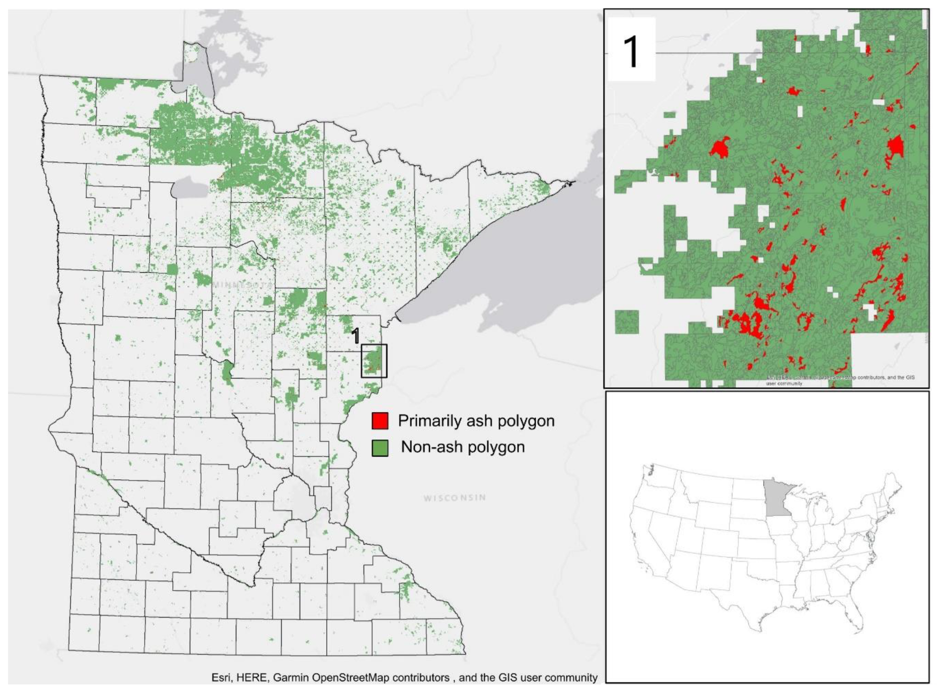
2.1.1. Study Area
2.1.2. Optical Imagery
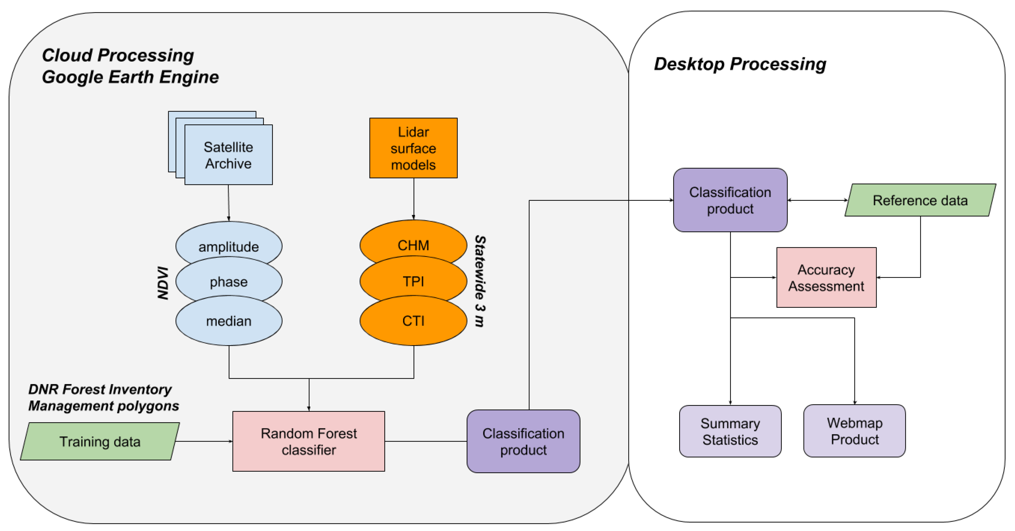
2.1.3. Google Earth Engine (Time Series)
2.1.4. Lidar
2.2. Model Development
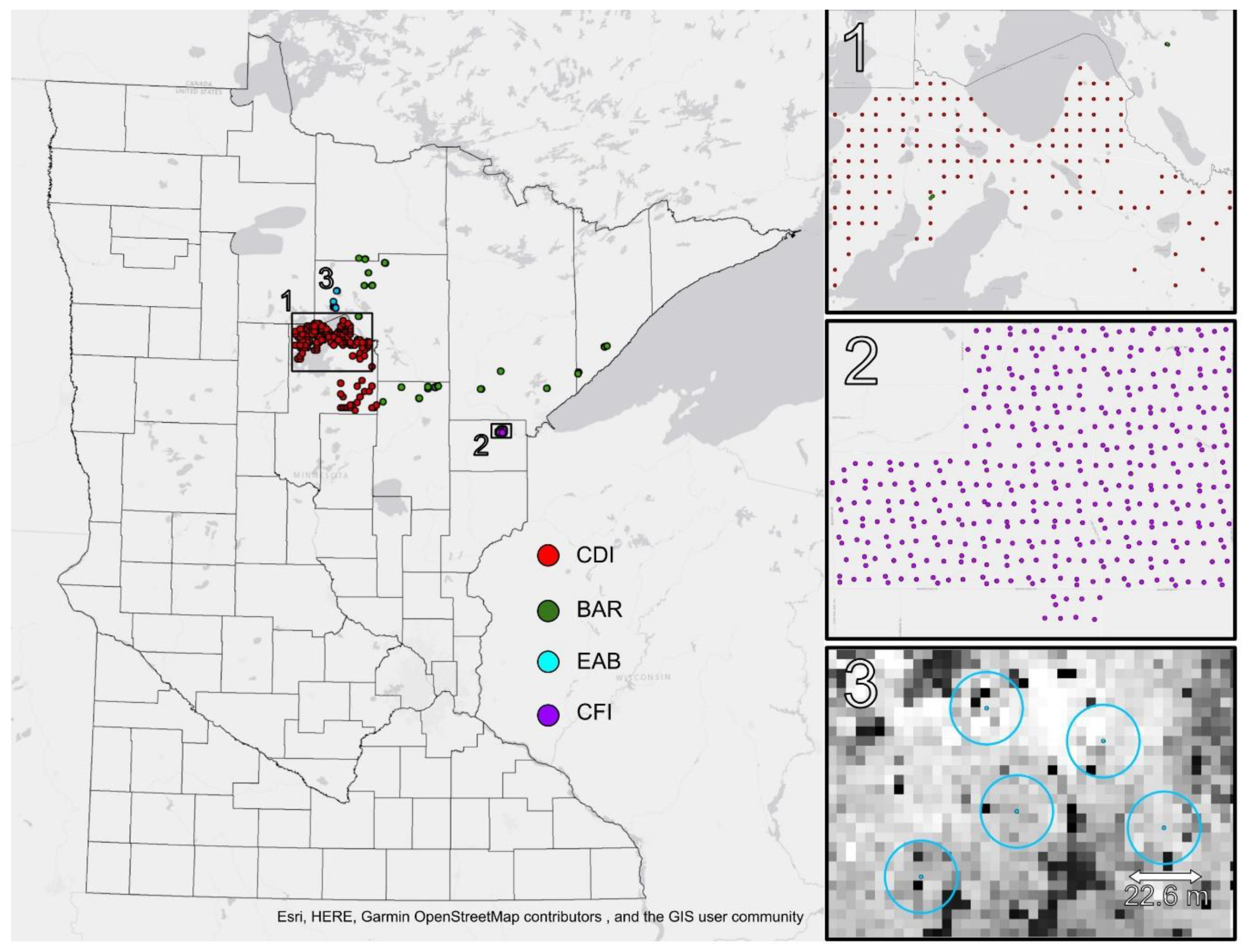
2.2.1. Forest Inventory Data
2.2.2. Basal Area Modeling
2.3. Model Validation
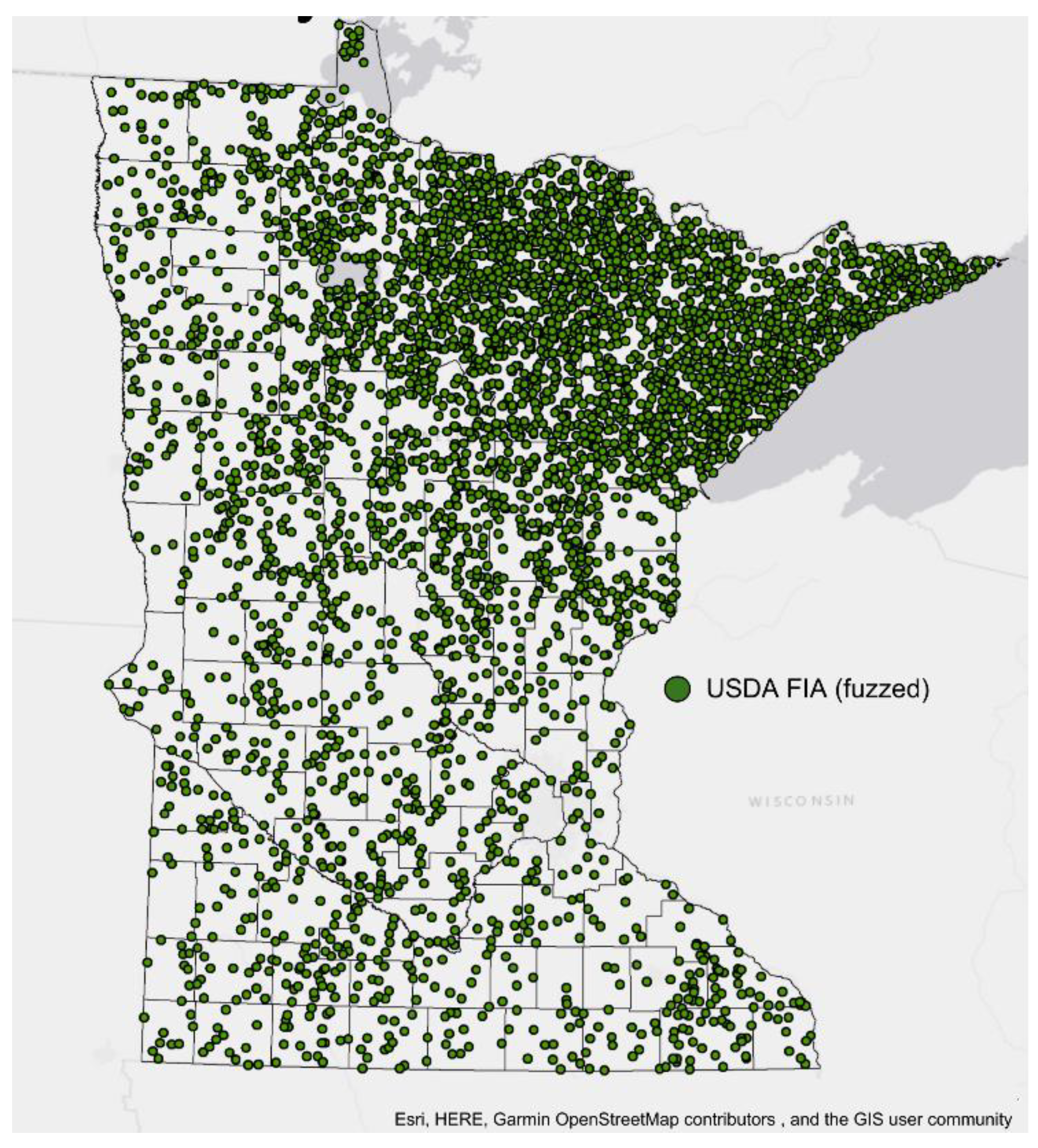
Forest Inventory and Analysis
3. Results
3.1. Ash Mapping
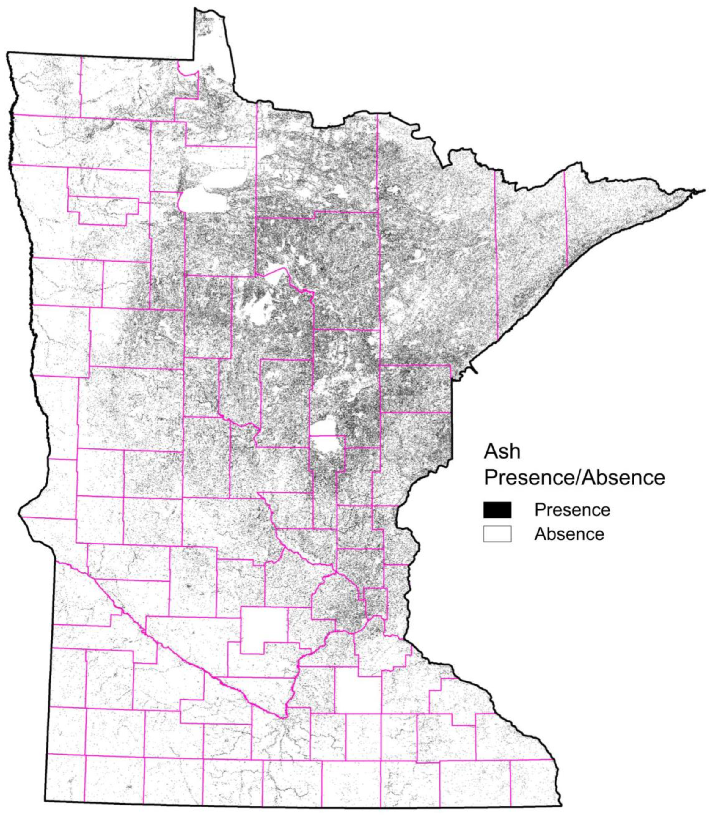
3.1.1. Ash Presence/Absence
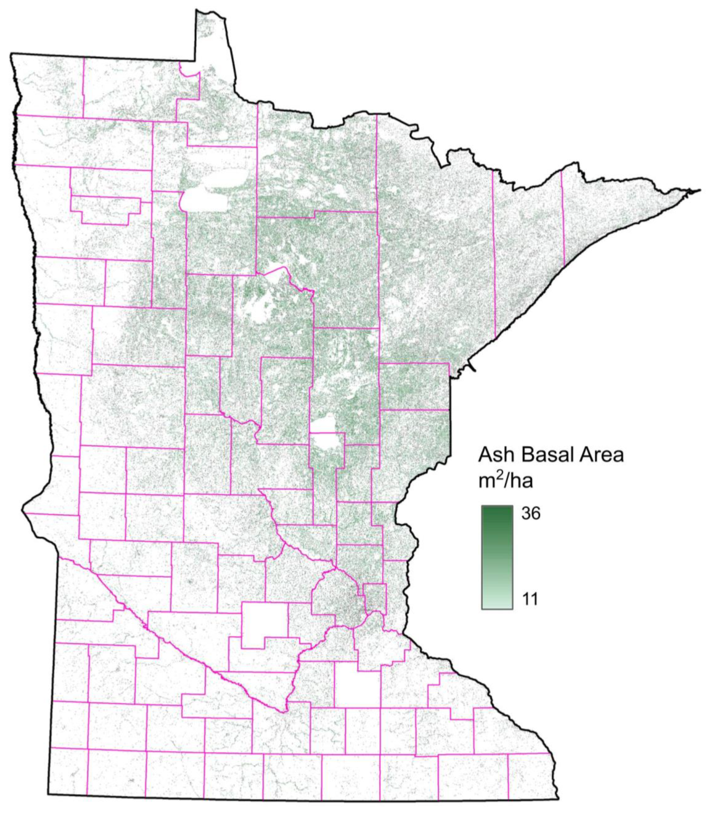
3.1.2. Ash Abundance
3.2. Validation
FIA Accuracy Assessment
4. Discussion
5. Conclusions
Author Contributions
Funding
Acknowledgments
Conflicts of Interest
References
- McRoberts, R.E.; Cohen, W.B.; Næsset, E.; Stehman, S.V.; Tomppo, E.O. Using remotely sensed data to construct and assess forest attribute maps and related spatial products. Scand. J. For. Res. 2010, 25, 340–367. [Google Scholar] [CrossRef]
- White, J.C.; Coops, N.C.; Wulder, M.A.; Vastaranta, M.; Hilker, T.; Tompalski, P. Remote sensing technologies for enhancing forest inventories: A review. Can. J. Remote Sens. 2016, 42, 619–641. [Google Scholar] [CrossRef]
- Lefsky, M.A.; Harding, D.; Cohen, W.B.; Parker, G.; Shugart, H.H. Surface lidar remote sensing of basal area and biomass in deciduous forests of eastern Maryland, MD, USA. Remote Sens. Environ. 1999, 67, 83–98. [Google Scholar] [CrossRef]
- Hudak, A.T.; Crookston, N.L.; Evans, J.S.; Hall, D.E.; Falkowski, M.J. Nearest neighbor imputation of species-level, plot-scale forest structure attributes from LiDAR data. Remote Sens. Environ. 2008, 112, 2232–2245. [Google Scholar] [CrossRef]
- McRoberts, R.E.; Tomppo, E.O. Remote sensing support for national forest inventories. Remote Sens. Environ. 2007, 110, 412–419. [Google Scholar] [CrossRef]
- Herms, D.A.; McCullough, D.G. Emerald ash borer invasion of North America: History, biology, ecology, impacts, and management. Annu. Rev. Entomol. 2014, 59, 13–30. [Google Scholar] [CrossRef]
- Morin, R.S.; Liebhold, A.M.; Pugh, S.A.; Crocker, S.J. Regional assessment of emerald ash borer, Agrilus planipennis, impacts in forests of the Eastern United States. Biol. Invasions 2017, 19, 703–711. [Google Scholar] [CrossRef]
- Miles, P.D.; VanderSchaaf, C.L.; Barnett, C.; Butler, B.J.; Crocker, S.J.; Gormanson, D.; Kurtz, C.M.; Lister, T.W.; McWilliams, W.H.; Morin, R.S.; et al. Minnesota forests 2013. In Res. Bull. NRS-104; USDA Forest Service, Northern Research Station: Newtown Square, PA, USA, 2016; p. 134. [Google Scholar]
- Kolka, R.K.; D’Amato, A.W.; Wagenbrenner, J.W.; Slesak, R.A.; Pypker, T.G.; Youngquist, M.B.; Grinde, A.R.; Palik, B.J. Review of ecosystem level impacts of emerald ash borer on black ash wetlands: What does the future hold? Forests 2018, 9, 179. [Google Scholar] [CrossRef]
- Kurtz, C.M.; Moser, W.K.; Hansen, M.H.; Gormanson, D.D.; Hatfield, M.A.; Sowers, P.A.; Dockry, M.J.; Emery, M.R.; Woodall, C.W.; Walters, B.F.; et al. Forest Resources within the Lake States Ceded Territories 1980–2013. In Resour. Bull. NRS-96; U.S. Department of Agriculture: Newtown Square, PA, USA, 2015; p. 89. [Google Scholar]
- Vogeler, J.C.; Slesak, R.A.; Fekety, P.A.; Falkowski, M.J. Characterizing over four decades of forest disturbance in Minnesota, MN, USA. Forests 2020, 11, 362. [Google Scholar] [CrossRef]
- Isaacson, B.N.; Serbin, S.P.; Townsend, P.A. Detection of relative differences in phenology of forest species using Landsat and MODIS. Landsc. Ecol. 2012, 27, 529–543. [Google Scholar] [CrossRef]
- Wilson, B.; Lister, A.; Riemann, R. A nearest-neighbor imputation approach to mapping tree species over large areas using forest inventory plots and moderate resolution raster data. For. Ecol. Manag. 2012, 271, 182–198. [Google Scholar] [CrossRef]
- Engelstad, P.S.; Falkowski, M.J.; D’Amato, A.W.; Slesak, R.A.; Palik, B.J.; Domke, G.M.; Russell, M.B. Mapping black ash dominated stands using geospatial and forest inventory data in northern Minnesota, USA. Can. J. For. Res. 2019. [Google Scholar] [CrossRef]
- Minnesota Department of Natural Resources. Ecological Classification System: Ecological Land Classification Hierarchy. Available online: https://www.dnr.state.mn.us/ecs/index.html (accessed on 17 February 2020).
- Rampi, L.; Knight, J.; Bauer, M. Minnesota Land Cover Classification and Impervious Surface Area by Landsat and Lidar: 2013 Update. Retrieved from the Data Repository for the University of Minnesota. Available online: https://conservancy.umn.edu/handle/11299/181555 (accessed on 17 February 2020).
- US Geological Survey Earth Resources Observation and Science Center. Landsat Collection 1 Level 1 Product Definition—Version 2.0. 2019, Retrieved from Sioux Falls, SD, USA. Available online: https://prd-wret.s3.us-west-2.amazonaws.com/assets/palladium/production/atoms/files/LSDS-1656_%20Landsat_Collection1_L1_Product_Definition-v2.pdf (accessed on 9 April 2020).
- Masek, J.G.; Vermote, E.F.; Saleous, N.; Wolfe, R.; Hall, F.G.; Huemmrich, F.; Gao, F.; Kutler, J.; Lim, T.K. LEDAPS Calibration, Reflectance, Atmospheric Correction Preprocessing Code; Version 2; ORNL DAAC: Oak Ridge, TN, USA, 2013. [Google Scholar] [CrossRef]
- US Geological Survey Earth Resources Observation and Science Center. Landsat 8 Surface Reflectance Code (LASRC) Product Guide—Version 2.0. 2019, Retrieved from Sioux Falls, SD, USA. Available online: https://prd-wret.s3.us-west-2.amazonaws.com/assets/palladium/production/atoms/files/LSDS-1368_L8_SurfaceReflectanceCode-LASRC_ProductGuide-v2.pdf (accessed on 9 April 2020).
- Foga, S.; Scaramuzza, P.L.; Guo, S.; Zhu, Z.; Dilley, R.D.; Beckmann, T.; Schmidt, G.L.; Dwyer, J.L.; Joseph Hughes, M.; Laue, B. Cloud detection algorithm comparison and validation for operational Landsat data products. Remote Sens. Environ. 2017, 194, 379–390. [Google Scholar] [CrossRef]
- Brooks, E.B.; Thomas, V.A.; Wynne, R.H.; Coulston, J.W. Fitting the multitemporal curve: A fourier series approach to the missing data problem in remote sensing analysis. IEEE Trans. Geosci. Remote Sens. 2012, 50, 3340–3353. [Google Scholar] [CrossRef]
- Shumway, R.H.; Stoffer, D.S. Time Series Analysis and Its Applications, with R Examples, 4th ed.; Springer: Berlin, Germany, 2017. [Google Scholar]
- Pasquarella, V.J.; Holden, C.E.; Kaufman, L.; Woodcock, C.E. From imagery to ecology: Leveraging time series of all available Landsat observations to map and monitor ecosystem state and dynamics. Remote Sens. Ecol. Conserv. 2016, 2, 152–170. [Google Scholar] [CrossRef]
- Moore, I.D.; Grayson, R.B.; Ladson, A.R. Digital terrain modelling: A review of hydrological, geomorphological, and biological applications. Hydrol. Proccess. 1991, 5, 3–30. [Google Scholar] [CrossRef]
- Breiman, L. Random forests. Mach. Learn. 2001, 45, 5–32. [Google Scholar] [CrossRef]
- Minnesota Department of Natural Resources. MNDNR Forest Stand Inventory. Available online: https://gisdata.mn.gov/dataset/biota-dnr-forest-stand-inventory (accessed on 7 April 2020).
- D’Amato, A.W.; Palik, B.J.; Slesak, R.A.; Edge, G.; Matula, C.; Bronson, D.R. Evaluating adaptive management options for black ash forests in the face of emerald ash borer invasion. Forests 2018, 9, 348. [Google Scholar] [CrossRef]
- Shrestha, M.; Wilson, D.C.; Zobel, J.M.; Ek, A.R. Cloquet Forestry Center Continuous Forest Inventory Update for 2014. University of Minnesota Department of Forest Resources Staff Paper Series no 243. 2016, p. 45. Available online: https://www.forestry.umn.edu/sites/forestry.umn.edu/files/staff_paper_243.pdf (accessed on 17 February 2019).
- R Core Team. R: A Language and Environment for Statistical Computing; R Foundation for Statistical Computing: Vienna, Austria, 2018. [Google Scholar]
- Fassnacht, F.E.; Latifi, H.; Stereńczak, K.; Modzelewska, A.; Lefsky, M.; Waser, L.T.; Straub, C.; Ghosh, A. Review of studies on tree species classification from remotely sensed data. Remote Sens. Environ. 2016, 186, 64–87. [Google Scholar] [CrossRef]
- Cohen, W.B.; Yang, Z.; Stehman, S.V.; Schroeder, T.A.; Bell, D.M.; Masek, J.G.; Huang, C.; Meigs, G.W. Forest disturbance across the conterminous United States from 1985–2012: The emerging dominance of forest decline. For. Ecol. Manag. 2016, 360, 242–252. [Google Scholar] [CrossRef]
- Wolter, P.P.; Townsend, P.A. Multi-sensor data fusion for estimating forest species composition and abundance in northern Minnesota. Remote Sens. Environ. 2011, 115, 671–691. [Google Scholar] [CrossRef]
- University of Minnesota Extension. Managing ash Woodlands: Recommendations for Minnesota Woodland Owners. University of Minnesota Extension. Retrieved from the University of Minnesota Digital Conservancy. Available online: http://hdl.handle.net/11299/205052 (accessed on 17 February 2019).
- Palik, B.J.; Ostry, M.E.; Venette, R.C.; Abdela, E. Fraxinus nigra (black ash) dieback in Minnesota: Regional variation and potential contributing factors. For. Ecol. Manag. 2011, 261, 125–135. [Google Scholar] [CrossRef]
- Asner, G.P.; Keller, M.; Pereira, R.; Zweede, J.C. Remote sensing of selective logging in Amazonia: Assessing limitations based on detailed field observations, Landsat ETM+, and textural analysis. Remote Sens. Environ. 2002, 80, 483–496. [Google Scholar] [CrossRef]


| Predictor | Resolution (m) | Abbreviation | Description | Source |
|---|---|---|---|---|
| NDVI Amplitude | 30 | NDVIa | Magnitude of NDVI difference 1 yr cycle | TM, ETM+, OLI, MSI |
| NDVI Phase | 30 | NDVIp | Day of year position of maximum NDVI | TM, ETM+, OLI, MSI |
| NDVI Median | 30 | NDVIm | Median of NDVI observations | TM, ETM+, OLI, MSI |
| Canopy Height Model | 3 | CHM | Max height of returns above ground level | ALS |
| Topographic Position Index | 3 | TPI | Local difference in elevation | ALS |
| Compound Topographic Index | 3 | CTI | Soil moisture potential calculated from a DEM | ALS |
| Dataset | Abbr | Plot Size (m2) | Year | Total n | Mean | SD | Min | Max |
|---|---|---|---|---|---|---|---|---|
| Ash basal area (m2/ha) | ||||||||
| Black ash research plots | BAR | 404 | 2018 | 80 | 18.62 | 6.63 | 0.00 | 41.21 |
| Chippewa-DNR inventory | CDI | 404 | 2017 | 147 | 23.44 | 14.55 | 0.36 | 68.81 |
| EAB research plots | EAB | 404 | 2015 | 42 | 28.92 | 6.53 | 9.54 | 48.71 |
| Cloquet forest inventory | CFI | 578 | 2014 | 349 | 23.93 | 12.81 | 0.25 | 72.42 |
| Sensor | Time Series | Time Series, TPI | Time Series, CTI | Time Series, TPI, CTI |
|---|---|---|---|---|
| Landsat 5 | 80% | 82% | 82% | 84% |
| Landsat 7 | 80% | 83% | 83% | 84% |
| Landsat 8 | 75% | 77% | 78% | 79% |
| Sentinel-2 | 78% | 81% | 80% | 81% |
| Time Series | Acquisition Years | Ash Detected | Ash Undetected | Total Ash Plots | Detection Accuracy |
|---|---|---|---|---|---|
| Landsat 5 | 1985–2011 | 573 | 684 | 1254 | 46% |
| Landsat 7 | 1999–present | 538 | 719 | 1254 | 43% |
| Landsat 8 | 2013–present | 470 | 787 | 1254 | 37% |
| Sentinel-2 | 2015–present | 369 | 888 | 1254 | 29% |
| Composite | 1985–present | 797 | 460 | 1254 | 64% |
| Source | Actual Presence | Actual Absence | Total | User’s Accuracy |
|---|---|---|---|---|
| Predicted presence | 797 | 1687 | 2484 | 32% |
| Predicted absence | 457 | 2981 | 3238 | 87% |
| Total | 1254 | 4668 | 5922 | - |
| Producer’s accuracy | 64% | 64% | - | 64% |
| Source | Ash Detected | Ash Undetected | Total Ash Plots | Detection Accuracy |
|---|---|---|---|---|
| All ash | 797 | 460 | 1254 | 64% |
| Black ash | 625 | 243 | 868 | 72% |
| Green ash | 267 | 237 | 504 | 53% |
© 2020 by the authors. Licensee MDPI, Basel, Switzerland. This article is an open access article distributed under the terms and conditions of the Creative Commons Attribution (CC BY) license (http://creativecommons.org/licenses/by/4.0/).
Share and Cite
Host, T.K.; Russell, M.B.; Windmuller-Campione, M.A.; Slesak, R.A.; Knight, J.F. Ash Presence and Abundance Derived from Composite Landsat and Sentinel-2 Time Series and Lidar Surface Models in Minnesota, USA. Remote Sens. 2020, 12, 1341. https://doi.org/10.3390/rs12081341
Host TK, Russell MB, Windmuller-Campione MA, Slesak RA, Knight JF. Ash Presence and Abundance Derived from Composite Landsat and Sentinel-2 Time Series and Lidar Surface Models in Minnesota, USA. Remote Sensing. 2020; 12(8):1341. https://doi.org/10.3390/rs12081341
Chicago/Turabian StyleHost, Trevor K., Matthew B. Russell, Marcella A. Windmuller-Campione, Robert A. Slesak, and Joseph F. Knight. 2020. "Ash Presence and Abundance Derived from Composite Landsat and Sentinel-2 Time Series and Lidar Surface Models in Minnesota, USA" Remote Sensing 12, no. 8: 1341. https://doi.org/10.3390/rs12081341
APA StyleHost, T. K., Russell, M. B., Windmuller-Campione, M. A., Slesak, R. A., & Knight, J. F. (2020). Ash Presence and Abundance Derived from Composite Landsat and Sentinel-2 Time Series and Lidar Surface Models in Minnesota, USA. Remote Sensing, 12(8), 1341. https://doi.org/10.3390/rs12081341