Abstract
This study proposes a hybrid intelligence approach based on an extreme gradient boosting regression and genetic algorithm, namely, the XGBR-GA model, incorporating Sentinel-2, Sentinel-1, and ALOS-2 PALSAR-2 data to estimate the mangrove above-ground biomass (AGB), including small and shrub mangrove patches in the Red River Delta biosphere reserve across the northern coast of Vietnam. We used the novel extreme gradient boosting decision tree (XGBR) technique together with genetic algorithm (GA) optimization for feature selection to construct and verify a mangrove AGB model using data from a field survey of 105 sampling plots conducted in November and December of 2018 and incorporated the dual polarimetric (HH and HV) data of the ALOS-2 PALSAR-2 L-band and the Sentinel-2 multispectral data combined with Sentinel-1 (C-band VV and VH) data. We employed the root-mean-square error (RMSE) and coefficient of determination (R2) to evaluate the performance of the proposed model. The capability of the XGBR-GA model was assessed via a comparison with other machine-learning (ML) techniques, i.e., the CatBoost regression (CBR), gradient boosted regression tree (GBRT), support vector regression (SVR), and random forest regression (RFR) models. The XGBR-GA model yielded a promising result (R2 = 0.683, RMSE = 25.08 Mg·ha−1) and outperformed the four other ML models. The XGBR-GA model retrieved a mangrove AGB ranging from 17 Mg·ha−1 to 142 Mg·ha−1 (with an average of 72.47 Mg·ha−1). Therefore, multisource optical and synthetic aperture radar (SAR) combined with the XGBR-GA model can be used to estimate the mangrove AGB in North Vietnam. The effectiveness of the proposed method needs to be further tested and compared to other mangrove ecosystems in the tropics.
1. Introduction
Intertidal mangrove forests are acknowledged as currently being one of the most important ecosystems worldwide due to the crucial services they provide to coastal populations, including food, fishery support, and blue carbon sequestration [1,2]. However, these forests are being lost worldwide due to anthropogenic threats, including overexploitation and conversion to aquaculture and agriculture, particularly in Southeast Asia and West Africa, despite multiple efforts at rehabilitation following international conservation strategies [3,4].
Mapping the spatial distribution and estimating the above-ground biomass (AGB) of mangrove forests and their carbon stock changes are often required to better understand and mitigate the driving factors and global loss of mangroves [5]. An accurate mangrove AGB retrieval is often required to assist in monitoring, reporting, and verification (MRV) schemes in climate change mitigation strategies such as blue carbon projects and the United Nations’ Reducing Emissions from Deforestation and Forest Degradation (REDD+) program in the tropics [6]. However, accurately mapping and estimating mangrove AGB remain challenging due to the complex structure of mangrove ecosystems, which consist of multiple species under different climate conditions in tropical and semi-tropical regions [7,8]. Field-based measured AGB or forest inventory approaches can accurately measure mangrove AGB. However, these methods include various disadvantages associated with the high cost of field measurements, the time-consuming nature of such methods, and site selection biases [9]. Therefore, the development of timely, precise, and cost-effective models to monitor mangrove AGB is needed to support mangrove restoration, conservation, and sustainable management.
In recent years, remote sensing-based approaches have been widely used to retrieve mangrove AGB and map carbon stocks using various sensors ranging from optical and synthetic aperture radar (SAR) to light detection and ranging (LiDAR) data [10,11,12] because such sensors provide a large number of benefits compared to traditional field-based methods such as lower cost, faster speed, easier repeatability, and the coverage of wider areas [13,14]. However, to date, there have been no attempts to investigate an integration of optical and SAR sensors, such as L-band, X-band, and C-band data, to retrieve the mangrove AGB using novel machine-learning (ML) techniques in tropical regions. Importantly, a current literature review indicates that mangrove AGB estimations have primarily been conducted for tall and dense mangrove forests (tree height > 2 m and diameter at breast high (DBH) > 5 cm) and have rarely been applied to shrub and small mangrove patches, resulting in deficiencies in total mangrove AGB estimations despite these forests being essential to coastal areas with respect to defending the coast against tidal waves and mitigating the effects of storm surges [15]. Accordingly, this study attempts to fill this knowledge gap by retrieving the mangrove AGB in the Red River mangrove biosphere reserve located in North Vietnam using an incorporation of Sentinel-1 and Sentinel-2 sensors fused with ALOS-2 PALSAR-2 data and ML models. We selected a combination of Sentinel-1 and Sentinel-2 multispectral instrument (MSI) data together with ALOS-2 PALSAR-2 because the Sentinel-1 C-band sensor may be useful to estimate small mangrove patches while the Sentinel-2 sensor has 13 spectral bands, which can be used to indicate the forest stand volume, and the longer L-band wavelength of the ALOS-2 PALSAR-2 sensor is able to penetrate tall mangrove canopies.
Prior studies indicate that empirical models applied to mangrove AGB estimations using remote sensing data are usually constructed using various regression techniques ranging from simple linear regression [16,17] and step-wise multi-linear regression models [18,19] to non-linear ML approaches [20,21,22]. A wide range of ML techniques has been proven to be useful for AGB retrievals of mangrove ecosystems using different Earth Observation (EO) data [23,24,25]. Non-parametric ML models, such as the random forest (RF) model [22,26], artificial neural network (ANN) models [21], and support vector machine (SVM) techniques [27], have increasingly been used for mangrove AGB retrievals with different EO datasets due to their ability to produce better prediction accuracies than parametric models. Recently, gradient boosting decision tree (GBDT) techniques have been shown to be powerful not only for classification but also for regression tasks, such as soil moisture estimation [28] and forest AGB estimation [29,30]. In particular, a novel GBDT technique, extreme gradient boosting regression (XGBR), which was proposed by Chen and Guestrin [31], outperforms other available boosting implementations when handling various environmental issues such as the mobility of disease [32], energy supply security [33], and lithology classification [34]. Despite its strong predictive performance and reliable identification of relevant features, however, the XGBR algorithm has rarely been used to retrieve mangrove AGB. Importantly, a quantitative comparison of available boosting and bagging decision tree techniques for the AGB retrieval of mangrove ecosystems in the biosphere reserves of Vietnam has not yet been reported in the literature.
In the present study, we propose a hybrid intelligence approach based on XGBR and the genetic algorithm (GA), namely, the XGBR-GA model, to estimate the mangrove AGB in the Red River Delta biosphere reserve (RRDBR) located in North Vietnam for the first time using ALOS-2 PALSAR-2 imagery together with an integration of Sentinel-1 and Sentinel-2 data. In addition, the performance of the XGBR model when retrieving the mangrove AGB is compared to that of other GBDT algorithms, i.e., the CatBoost regression (CBR) and gradient boosted regression tree (GBRT) algorithms, as well as two well-known ML algorithms, the support vector regression (SVR) and random forest regression (RFR) models. Our results show the potential use of the XGBR-GA-based model for mangrove AGB retrieval using an incorporation of Sentinel-1 and Sentinel-2 data combined with ALOS-2 PALSAR-2 data to improve the prediction accuracy of mangrove AGB estimations in biosphere reserves including small and shrub mangroves in the tropics to better support sustainable conservation and the management of mangroves.
2. Materials and Methods
2.1. Study Site
The present study was conducted in three different mangrove ecosystems across the northern coast of Vietnam, which consists of three coastal provinces, Nam Dinh, Thai Binh, and Hai Phong. The geographical coordinates of the region are 20°00′–21°04′ N and 106°01′–106°50′ E. The study area is located on the western coastal zone of the Gulf of Tonkin and lies in the Red River Delta (Figure 1), which was adopted as a biosphere reserve by the United Nations Educational, Scientific, and Cultural Organization in 2004. Of the three coastal regions in the Red River Delta, the Xuan Thuy National Park is located in Nam Dinh Province and was the first Ramsar site designated in Vietnam in 1982 [35]. The climate of the study area consists of a sub-tropical and semi-tropical monsoon with two seasons. The dry season starts in October and ends in the following March, whereas the rainy season begins in April and lasts until September. The average temperature is approximately 23 °C, the annual rainfall is roughly 1300–1400 mm, and the humidity is approximately 80% [36]. The mangrove ecosystems of the Red River Delta are diverse and are distributed between zones I and II of the four Vietnamese mangrove zones [37] and consist of the second largest mangrove forest in the country (Figure 1).
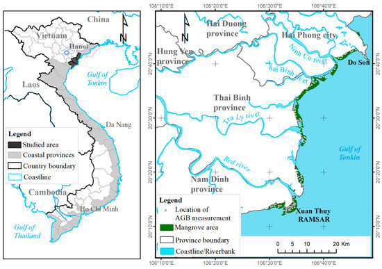
Figure 1.
Location map of the mangrove study areas.
The mangrove ecosystems consist of the intertidal mangrove forests and their adjacent areas, which form a transitional zone between the aquatic and terrestrial regions. There are approximately 10 mangrove species found in the coastal zones, of which the most dominant species are Rhizophora stylosa, Kandelia obovata, Aegiceras corniculatum, Bruguiera gymnorrhiza, Avicennia marina, and Sonneratia caseolaris [38].
2.2. EO and Field Survey Data Collection
2.2.1. Satellite Remotely Sensed Data
We employed data from three different EO sensors including the Advanced Land Observing Satellite-2 Phased Array type L-band Synthetic Aperture Radar-2 (ALOS-2 PALSAR-2) Level 2.1 with highly sensitive dual polarimetric modes at the horizontal transmitting and horizontal receiving (HH) and the horizontal transmitting and vertical receiving (HV) polarizations and the Sentinel-2 (S-2) Level 1C MSI together with the Sentinel-1 (S-1) Level-1 Ground Range Detected (GRD) product with C-band (Vertical transmit-Vertical receiving (VV) and Vertical transmit-Horizontal receiving (VH) dual polarization) data to estimate the mangrove AGB at mangrove areas in the RRDBR. The ALOS-2 PALSAR-2 imagery was acquired on October 18, 2018, whereas the S-2 MSI and S-1 SAR data were acquired on November 2 and 5, 2018, respectively (Table 1). The eleven multispectral bands of the S-2 with spatial resolutions ranging from 10 to 20 m were used, including coastal band 1 (443 nm) together with three visible bands, i.e., Blue (492 nm), Green (560 nm), and Red (665 nm), near-infrared (NIR) (832 nm), narrow-NIR (865 nm), three red-edge bands (704 nm, 740 nm, 783 nm), and two short-wavelength infrared (SWIR) bands (1614 nm–2202 nm) [39].

Table 1.
The EO remotely sensed data used in this study.
The S-1 dual polarimetric C-band in high resolution for the Interferometric Wide Swath (IW, 250 km swath width) for the VV and VH polarization data Level 1 GRD mode and the S-2 MSI Level 1C data were downloaded from the Copernicus Open Access Hub (https://scihub.copernicus.eu) run by the European Space Agency (ESA), whereas the ALOS-2 PALSAR-2 data for the HH and HV dual polarimetric data Level 2.1 were acquired from the Japan Aerospace Exploration Agency (JAXA).
2.2.2. Data Collection from the Mangrove Inventory
We conducted a mangrove forest inventory with permission from the local authorities during the lowest tidal levels in November and December 2018, similar to remote sensing data acquisitions during the dry season in North Vietnam. A total of 105 plots were measured using a stratified random sampling approach, in which each sampling plot was defined using an initial survey and the support of locals to guarantee that the AGB ranges would be usable for the all of the mangrove ecosystems across the RRDBR. In each plot, we measured different biophysical parameters, including the tree height (H), DBH, canopy diameter (CD), and diameter at 30 cm above the root system (D30) for Rhizophora stylosa as suggested by Clough and Scott [40]. The biophysical parameters of all the mangrove forest stands, including small and shrub mangrove patches, in a sampling plot within 10 m × 10 m (0.01 ha) were measured.
We measured the crown diameter of a shrub mangrove tree using Equation (1) since its crown area was considered to be a circle or an ellipse.
where W1 is the widest length of the tree canopy through its center, and W2 is the canopy width perpendicular to W1.
We used a Garmin eTreX global positioning system with an accuracy of ±2 m to record the location of the sampling plot. Figure 2 shows the techniques used to measure the biophysical parameters of the different mangrove species.
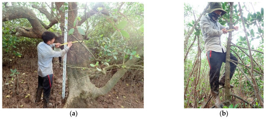
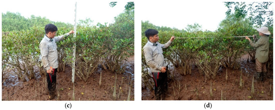
Figure 2.
Mangrove AGB measurements of different species in the biosphere reserve: (a,b) biophysical parameter measurements (DBH and H) of tall mangroves and (c,d) crown diameter (CD) measurements of shrub mangrove patches. (Photos were taken by T.D. Pham in November and December of 2018.).
The dry AGB for each mangrove species was calculated using the allometric equations. The allometric methods are non-destructive approaches, which have been widely used to estimate mangrove AGB, involving the establishment of a relationship between the mangrove biomass and several biophysical parameters shown in Table 2 [40,41,42]. We also measured all shrub and small mangrove stands with DBH values of less than 5 cm and tree heights of less than 2 m to calculate their AGB using the appropriate allometric equations (Table 2).
Table 2.
Allometric equations for each mangrove species in the study area.
3. Methods
We propose a novel framework using an advanced ML technique combined with multiple source EO data for mangrove AGB estimations; our technique consists of the following steps: (1) pre-processing and processing of multiple source EO data (SAR and optical data); (2) integrating the ground truth collected from field surveys with EO data extraction to create training and testing datasets; (3) testing and comparing the ML model performances using all the features; and (4) selecting the optimal variables and optimizing the hyperparameters using GA based on cross-validation and re-evaluating the results using the optimal variables for mangrove AGB estimations in the RRDBR (Figure 3).
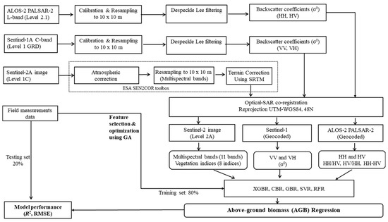
Figure 3.
Flowchart for processing the satellite images and generating mangrove AGB predictive models using the ML techniques covered in this study.
3.1. Satellite Image Processing
The ALOS-2 PALSAR-2 Level 2.1 dual polarization data during the dry season in North Vietnam from JAXA were converted to the backscattering coefficient using Equation (2):
where DN is the digital number of the amplitude image; σ0 is the backscattering coefficient; and CF is the calibration factor. Note that CF = −83 dB was applied for the dual polarimetric SAR data [43]. The DN of each pixel was converted to σ0 in decibel (dB) units.
σ0 [dB] = 10 × log10 (DN)2 + CF
The S-2 Level-1C and the S-1 GRD products for the study area during the dry season were downloaded from the Copernicus Open Access Hub, ESA. The top-of-atmosphere reflectance of S-2 [39] was converted to the Level 2A bottom-of-atmospheric reflectance after geometric and atmospheric corrections using the ESA Sen2Cor algorithm [44]. The S-1 C-band image intensities at the VV and VH polarizations were processed in multiple steps, including thermal noise removal, calibration, despeckling, terrain correction, and finally conversion to the normalized radar σ0 in decibel (dB) units [45]. Then, the S-2 data were co-registered with the S-1 and ALOS-2 PALSAR-2 data in the UTM/WGS84 coordinate system at the zone 48N projection. Since the three sensors acquire data at different spatial resolutions (Table 1), we resampled all data to a ground sampling distance (GSD) of 10 m to match the size of a sampling plot of 100 m2. The three sensors were resampled during the pre-processing step before co-registering three sensors (Figure 3). The SNAP toolbox was used to process the S-1, S-2, and ALOS-2 PALSAR-2 data.
3.2. Image Transformation of the S-2 Multispectral and ALOS-2 PALSAR-2 Imagery
Image transformations for optical and SAR data have commonly been applied in mangrove AGB retrievals in previous studies [7,11,19]. In this study, we employed an SAR image transformation for the ALOS-2 PALSAR-2 imagery consisting of a combination of multi-polarizations [21] and used eight vegetation indices (VIs) of the S-2 MSI data, as shown in Table 3, because each index is sensitive to the mangrove structure and biomass [29,46,47]. For instance, the ratio vegetation index (RVI) is effective for retrieval of the mangrove structure [48]. The normalized difference vegetation index (NDVI) has been widely used for mangrove AGB as it is strongly correlated with mangrove biophysical parameters [49]. Further, enhanced vegetation index-2 (EVI-2) is relatively sensitive to mangrove AGB [50,51]. Additionally, the soil-adjusted vegetation index (SAVI) was also computed in this study because soil brightness at low vegetation cover is correlated with forest structure [52,53]. Importantly, some potential vegetation indices derived from the red-edge bands of S-2, such as the normalized difference index using bands 4 & 5 of S-2 (NDI45), inverted red-edge chlorophyll index (IRECl), and modified chlorophyll absorption in reflectance index (MCARI), have been frequently used for forest AGB estimation in recent studies because of their excellent explanations of the relationship between biophysical parameters and forest AGB [54,55].
Table 3.
List of the vegetation indices used in the current study.
We chose a total of 26 predictor features consisting of 11 multispectral bands of S-2 and 8 VIs derived from S-2, 5 variables (HH, HV, HH/HV, HV/HH, and HH-HV) derived from the ALOS-2 PALSAR-2 data and two backscattering coefficients (VV and VH) from S-1 (Table 3) to generate inputs for the mangrove AGB estimation model. All of the predictor variables were normalized using the normalization function in the Scikit-learn library in the Python environment [63].
3.3. Machine Learning Models Used
In this study, we present a hybrid approach based on XGBR and GA to estimate the mangrove AGB in the RRDBR. To confirm the effectiveness of the proposed model for mangrove AGB estimation, the predictive performance of the model was compared to other existing state-of-the-art GBDT models, i.e., CBR and GBR, and the RFR and SVR models as baselines. The SVR model was selected because it produced the best prediction performance of the various ML techniques when retrieving the mangrove AGB in a coastal area in North Vietnam [8]; the RF model was selected because it outperformed other techniques for mapping and modeling the mangrove AGB change in South Vietnam [22]. The other GBDT models represent the most widely used methods for robust regression problems in several fields, as reported in recent studies [32,64,65]. In the current study, we determined the optimal hyperparameters of each ML algorithm using the grid search with a 5-fold CV in the Python environment.
3.3.1. Gradient Boosting Decision Tree (GBDT) Algorithms
GBDT is a popular ML algorithm using the ensemble-based decision tree method, which was developed by Friedman [66]. The GBDT model first builds decision trees from original data with equal weights. Then, the result is assessed, giving a higher weight to variables that are difficult to classify and a lower weight to variables that are easy to classify. The GBDT model improves the accuracy of the prediction using additional subsequent trees and evaluates the accuracy using a loss function. Importantly, the GBDT algorithm optimizes the loss function and makes a prediction from a weak supervised learner (decision tree) and then adds new decision trees to minimize the loss function [67]. GBDT models can handle mixed types of data for both classification and regression tasks. These techniques often perform feature selection and are robust against outliers [68]. GBDT models, however, have not been widely applied to mangrove AGB retrieval. Therefore, we employed several different state-of-the-art GBDT techniques, i.e., the XGBR, GBRT, and CBR algorithms, for the mangrove AGB estimation in the current study.
1. Extreme Gradient Boosting Regression (XGBR)
The XGB algorithm is a relatively new technique that belongs to the gradient boosting machine family, which was proposed by Chen and Guestrin [31]. This algorithm can handle both classification and regression tasks for weak supervised learning in machine learning via additive training strategies. The XGB technique aims to overcome the overfitting problem and optimize performance and has recently won multiple ML competitions [69].
In the XGB benchmark, the process of additive learning is divided into two phases. The first learning phase is fitted to the entire input dataset, whereas the second phase is fitted to the residuals to resolve the drawbacks of weak supervised learning. The fitting process is repeated multiple times until the stopping criteria are achieved. The XGB algorithm requires a large number of hyperparameters that must be selected and tuned beforehand. Therefore, in the present study, we used a GA to automate the tuning of the hyperparameters and optimal feature selection to improve the model performance.
2. Gradient boosting regression trees (GBRT)
The gradient boosting machine (GBR) algorithm was first introduced by Friedman [67]. The GBRT technique, which belongs to the stochastic gradient boosting family, can fit different types of data distributions, such as Gaussian, Poisson, Bernoulli, or binomial. GBRT models can handle interactions and automatically generate the feature importance and are robust to various correlated and irrelevant predictor variables, as well as outliers [70]. In the GBRT technique, a predictor variable is selected for splitting and then weighted in the model a certain number of times by the squared increment. Then, the contribution or relative importance of each variable is scaled and assigned to a number, where higher numbers reflect a stronger influence on the model [67].
3. CatBoost regression (CBR)
CBR is a novel gradient boosting technique that was recently developed by Dorogush, et al. [71]. This algorithm can handle both classification and regression problems and has been released in a new open-source gradient boosting library [71,72]. The CBR model uses the decision tree as the base weak learner and gradient boosting to iteratively fit a sequence of such trees. In the CBR model, the random permutations of the training dataset and the gradients used for choosing an optimal tree structure are generated to enhance the robustness of the algorithm and prevent overfitting [71].
Note that the learning efficiency of the CBR algorithm is controlled by its model hyperparameters, including max_depth, learning_rate, and the number of iterations. The selection of the optimal hyperparameters is a challenging task and may be time-consuming depending on the user’s experience.
3.3.2. Support Vector Regression (SVR)
The SVM algorithm is a supervised learning technique based on statistical learning theory, which was developed by Vapnik [73]. This method is widely used for classification and forecasting in data analysis, computer vision, and pattern recognition. SVR belongs to the SVM algorithm family and is commonly used for solving regression problems. The performance of the SVR model is highly influenced by the choice of the various kernel functions. To minimize the bias, the radial basis function (RBF) kernel was used in the current study because it has been applied to forest biophysical parameter retrievals in prior studies [11,47].
The quality of the mangrove AGB retrieval can be evaluated by the ε insensitive loss function developed by Vapnik [73]. In the SVR model, three parameters are often needed to configure a model with an RBF kernel: (1) the regularization parameter (C), which makes the trade-off between the model complexity and the training errors; (2) ε, which defines the allowed errors for each training data sample; and (3) γ, which is a parameter of the RBF kernel.
3.3.3. Random Forest Regression (RFR)
RF [74] is currently the most common bagging method in use; RF uses ensemble decision trees and works effectively for both classification and regression problems. The RF algorithm creates multiple uncorrelated trees for the training, using a random subset of two-thirds of the total sample, and leaves one-third of the total sample (out-of-bag (OOB)) for the validation. The samples are randomly collected with a replacement of the samples in the collection numbers. A tree is grown using in-bag samples with m variables to define the optimal split for each node. A tree can be grown to its largest extent in the case where no pruning is applied. The model produces the OOB error and the variable importance to assess the prediction accuracy and indicate the contribution of each variable. The RFR model is a well-known method that has been widely used in forest AGB estimations in previous studies [22,75].
In an RFR model, two parameters, the number of trees and the number of features used for the split, need to be determined.
3.4. Model Configuration, Implementation, and Assessment
3.4.1. Model Configuration and Training
The configuration and training of the five ML models were conducted using a training dataset in Python 3.7. A total of 105 sampling plots were divided such that 80% were included in the training set and 20% were included in the testing set to assess the performance of the models using the Scikit-learn library [63]. We used a median filter with a moving window size of 7 × 7 pixels in the SciPy library [76] to reduce the effect of the SAR, such as the ALOS-2 PALSAR and S-1 images, and the optical noise, as suggested by previous studies [21,47].
3.4.2. Hyperparameter Tuning of XGBR, CBR, GBRT, RFR, and SVR.
Table 4 shows the optimal hyperparameter values of each ML model using all the features derived from S-1, S-2, and ALOS-2 PALSAR-2.
Table 4.
Prior hyperparameter tuning using a grid search with a 5-fold CV for the different ML techniques.
We first tested the ML models with all features (predictor variables) with applied hyperparameter tuning using a grid search with a 5-fold CV (Table 4). Based on the highest predictive performance, i.e., the lowest root-mean-square error (RMSE), we selected the best model. Then, we used the GA with the highest predictive model to select the optimal features using different combinations (scenarios) derived from the S-1, S-2, VI, and ALOS-2 PALSAR-2 data for the mangrove AGB estimation in terms of the coefficient of determination (R2) and the RMSE. Finally, we tested all selected ML models with the optimal features for comparison.
3.4.3. GA for Feature Selection
Optimal feature selection using the GA was implemented to automatically identify the optimal variables for AGB retrieval in the RRDBR. The GA uses the idea from the Darwinian theory for natural selection in evolution by employing the computer capacity to automate the tuning of a number of parameters in an ML model [77]. The most important concept of GA is the chromosome, which consists of ML model parameters that define a solution (called an individual).
The basic operation performed during the training of the machine learning model consists of the following steps: (1) a total number of 105 samples (individuals) are initialized to form a population, (2) individuals with the best fitness values are selected to generate a mating pool, (3) from the mating pool, parents are selected by either sequential or random selection methods, and (4) several operators called crossover and mutation operators are then applied to each pair of parents to generate their offspring. This process retains high-quality individuals to generate more individuals, therefore evolving the solutions to obtain the desired solutions. We implemented the GA in the Python 3.7 environment to select the optimal features together with the hyperparameters in terms of RMSE and R2 using a 5-fold CV technique.
3.4.4. Model Evaluation
We employed RMSE and R2 to evaluate and compare the model performances of the five ML algorithms used in this study because these statistical measures are commonly used in modeling forest AGB. These indices are often employed to evaluate the differences between the measured AGB and the predicted AGB data [47] because RMSE (Equation (3)) and R2 (Equation (4)) are standard criteria used to measure statistical errors in regression models. Higher R2 and lower RMSE values indicate better performance for an ML model [11,16]. We employed Scikit-learn in Python 3.7 to evaluate the performances of all the ML models in the current study [78].
where is the estimated mangrove AGB value from the ML model, is the measured mangrove AGB value obtained from the field survey, n is the total number of sampling plots, and and are the mean values of the estimated mangrove AGB and the measured mangrove AGB, respectively.
4. Results
4.1. Mangrove Tree Characteristics in the RRDBR
All mangrove forest stands, including small and shrub mangrove patches, were measured in 105 sampling plots in mangrove areas across three coastal districts of the RRDBR (Figure 1). The characteristics of the mangrove trees are described in Table 5 and show mangrove AGB values ranging from 2.71 Mg·ha−1 to 257.08 Mg·ha−1. The mean AGB values range between 51.58 Mg·ha−1 and 79.90 Mg·ha−1. Of the three coastal provinces in the RRDBR, the mean mangrove AGB values measured in Thai Binh and Hai Phong provinces were slightly higher than those measured in Nam Dinh Province. The mangrove heights in Nam Dinh varied from 0.6 m to 7.5 m, and their DBHs ranged from 2.2 cm to 11.5 cm, whereas these corresponding numbers were relatively higher, varying from 1.1 m to 14.8 m with the mangrove heights and from 2.7 cm to 23.8 cm with their DBHs in Thai Binh and Hai Phong. The mangrove tree densities in Nam Dinh ranged from 315 to 8285 tree·ha−1, which were much higher than those in Hai Phong and Thai Binh provinces, ranging from 198 to 6434 tree·ha−1.
Table 5.
Characteristics of the mangrove trees in the RRDBR.
4.2. Modeling Results, Assessment, and Comparison
Table 6 shows the performances of the five ML techniques using all the features derived from S-1, S-2, the VIs, and ALOS-2 PALSAR-2. It can clearly be seen that the XGBR model yielded the highest predictive performance in the testing phase (R2 = 0.622 and RMSE = 27.39 Mg·ha−1), followed by the GBRT model (R2 = 0.563 and RMSE = 33.75 Mg·ha−1). Conversely, the RFR model produced the lowest performance (R2 = 0.426 and RMSE = 33.75 Mg·ha−1).
Table 6.
ML technique performance using all the features for the mangrove AGB retrieval in this study.
The results in Table 6 reveal that, of the five ML models, the best predictive performance was observed for the XGBR algorithm (Table 6) using all the features derived from a combination of the S-2 (11 MS bands), S-1 (2 bands), ALOS- 2 PALSAR-2 (5 bands), and VI (8 bands) data (Table 7). The XGBR model yielded a good R2 of 0.622 for the testing set and an RMSE of 27.39 Mg·ha−1. The RMSE achieved by the XGBR model is much lower than the average standard deviation obtained from the AGB field-based measurement (37.96 Mg·ha−1), reflecting a goodness-of-fit between the model estimation and the actual field survey measurements.
Table 7.
Performance of the XGBR model with different numbers of features.
We also computed six scenarios (SCs) using different combinations derived from the S-2, S-1, ALOS-2 PALSAR-2, and VIs datasets to test the performance of the XGBR model for mangrove AGB retrieval. The performance of each scenario is shown in Table 7.
It can be clearly seen in Table 7 that the XGBR-based model produced the highest accuracy using the 19 selected features in SC5 optimized by the GA. The 19 optimal features consist of eight MS bands (bands 1, 4, 5, 6, 7, 8, 11, and 12) from S-2, 5 VIs (NDVI, NDI45, SAVI, EVI-2, and IRECl), four bands from ALOS-2 PALSAR-2 (HV, HH/HV, HV/HH, and HH-HV), and two bands from S-1 (VV and VH). The XGBR model achieved a promising result with R2 values of 0.990 and 0.683 for the training and testing sets, respectively, and an RMSE of 25.08 Mg·ha−1. In addition, the result using the 19 optimal features was relatively better than that using all the features (the 26 predictor variables), with an increase of 0.061 for R2 during the testing phase and a decrease of 2.31 Mg·ha−1 for RMSE. Contrastingly, a combination of just the S-2 and VI datasets had the lowest performance (R2 = 0.378 in the testing set and RMSE = 48.24 Mg·ha−1), followed by combinations of only the ALOS-2 PALSAR-2 and S-1 datasets (R2 = 0.302 in the testing set and RMSE = 37.20 Mg·ha−1) and the S-2 dataset alone (R2 = 0.301 in the testing set and RMSE = 34.14 Mg·ha−1).
The data from SC5 were used to re-evaluate the performances of the XGBR, CBR, GBRT, SVR, and RFR models. Our results indicate an improvement in the R2 and a reduction in the RMSE with respect to the XGBR-GA model (Table 8). Noticeably, the three GBDT algorithms (XGBR, GBRT, and CBR) showed acceptable results in mangrove AGB retrieval with R2 values ranging from 0.587 to 0.683 in the testing set and RMSE values ranging from 25.08 Mg·ha−1 to 28.62 Mg·ha−1, which was significantly lower than the standard deviation of 37.96 Mg·ha−1 observed by the AGB field-based measurement (Table 3), showing that the GBDT algorithms work well and outperform the SVR and RFR algorithms for mangrove AGB retrieval in the study area.
Table 8.
Comparison of the model performances using new predictor variables based on the GA.
In SC5, a combination of the 19 optimal features derived from the S-2 MSI (involving the VI bands) and S-1 together with the ALOS-2 PALSAR-2 data boosted the R2 value to 0.683 with a lower RMSE of 25.08 Mg·ha−1. The results in the testing phase (Figure 4) indicate a better predictive performance with a higher R2 and a lower RMSE observed for the mangrove AGB estimation. Overall, the XGBR-GA model produced the best performance for the mangrove AGB estimation in the study area.
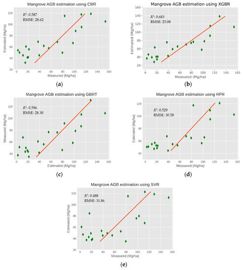
Figure 4.
Comparison of the predictive performances of the ML methods for mangrove AGB estimations using multi-sensors in the testing phase. (a) CBR, (b) XGBR, (c) GBRT, (d) RFR, (e) SVR.
4.3. Variable Importance
The results in Figure 5 reveal that, of the eight multispectral bands of S-2 MSI selected by the GA algorithm, the shortwave infrared (SWIR-1) band (band 11 at 1610 nm) and the NIR spectrum (band 8 at 845 nm) were the most sensitive to mangrove AGB, followed by the SWIR-2 band (band 12 at 2202 nm) and two red-edge-1 and -2 spectra (band 5 at 704 nm and band 6 at 740 nm). These results indicate that the VIs derived from the NIR and the RED reflectance, such as NDVI and EVI-2, play a less important role in mangrove AGB retrieval than the polarization computed from ALOS-2 PALSAR-2 imagery such as HH-HV. Interestingly, we found that, of the VI indices, the inverted red-edge chlorophyll index (IRECl) and the normalized difference index (NDI45) using bands 4 and 5 of S-2 were strongly correlated with the mangrove AGB in the study area. This study also indicates that the band ratios derived from the incorporation of dual polarimetric SAR data from ALOS-2 PALSAR-2 imagery such as HH/HV and HV/HH were relatively important for estimating the mangrove AGB in the biosphere reserve. Of the four polarimetric modes of S-1 and ALOS-2 PALSAR-2, backscatter coefficients derived from cross-polarization HV were found to be the most sensitive to mangrove AGB at the study site. Two backscatter coefficients of the S-1 sensor were selected in the final XBGR model. However, their contributions were much smaller than those of the ALOS-2 PALSAR-2 imagery.
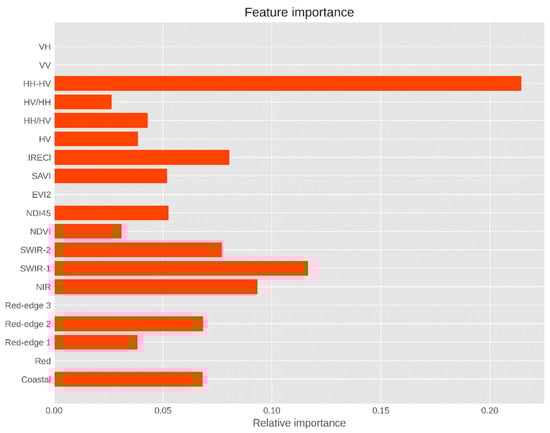
Figure 5.
Variable importance of the S-2, S-1, and ALOS-2 PALSAR-2 data in the present study.
4.4. Generation of Mangrove AGB Maps in the Study Area
Because the XGBR-GA model produced the best prediction performance and outperformed the remaining ML algorithms using data fusion derived from S-1, S-2, the VIs, and the ALOS-2 PALSAR-2 sensors in the RRDBR, this model was chosen for mangrove AGB retrieval in the current study. The final results were converted to raster GeoTIFF format and then visualized in QGIS for each coastal province in North Vietnam. The mangrove AGB map was interpreted according to six classes (Figure 6), ranging from 17 Mg·ha−1 to 142 Mg·ha−1 (with an average of 72.47 Mg·ha−1).
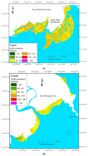
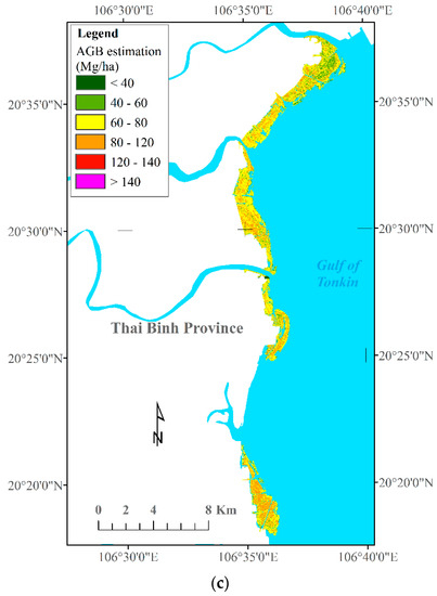
Figure 6.
Mangrove AGB estimation maps across the three studied coastal areas in the RRDBR. (a) Nam Dinh—Ramsar site, (b) Hai Phong, (c) Thai Binh.
Figure 6 shows the mangrove AGB maps with the spatial distribution patterns in the three studied coastal zones of the RRDBR. As can be seen from Figure 6, the highest biomass value was found in the core zone of the biosphere reserve, primarily at the Ramsar site, and in the deltas of the Red and Thai Binh rivers, whereas the lowest biomass values were observed next to the sea. Despite the goodness-of-fit between the mangrove AGB values generated by the XGBR-GA model and the actual measured mean values, the mean estimated mangrove AGB value (72.47 Mg·ha−1) was higher than the actual mean field-based measurement (62.75 Mg·ha−1) (Table 3).
5. Discussion
Over the past 10 years, various attempts have been made to obtain mangrove AGB estimations using simple linear regression [79] and multi-linear regression [18,19,80]; these attempts resulted in low performance with R2 values ranging from 0.43 to 0.65. In recent years, ML algorithms such as Gaussian process regression, multi-layer perception neural networks, SVR, and RFR techniques have been employed to retrieve mangrove AGB, as reported in a number of published case studies [8,20,21,22]. ML techniques often achieve better predictive performances compared to conventional parametric methods for mangrove AGB retrievals [20,81]. However, to date, an estimation of mangrove AGB including shrub and small mangrove patches has not been reported in the literature, indicating a need to propose an alternative and new approach to mangrove AGB estimation to support MRV and blue carbon projects. Here, we proposed a hybrid approach based on the XGBR-GA model using an incorporation of ALOS-2 PALSAR-2, S-1, and S-2, and VI data and achieved a satisfactory result (R2 = 0.683, RMSE = 25.08 Mg·ha−1) for forest AGB retrieval in the RRDBR across three coastal provinces in North Vietnam. The modeling results of the mangrove AGB retrieval in the RRDBR using the different ML techniques (XGBR, CBR, GBRT, SVR, and RFR) revealed that the XGBR-GA model had the highest predictive performance and outperformed the other ML models with R2 and RMSE values of 0.683 and 25.08 Mg·ha−1, respectively (Table 8). Using the GA for the XGBR model in this study, the performance improved with an R2 increase of 0.061. Conversely, the SVR model showed the lowest performance with R2 and RMSE values of 0.488 and 31.86 Mg·ha−1, respectively. Note that the CBR model (R2 = 0.587) and the GBRT model (R2 = 0.596) are relatively good predictors for mangrove AGB retrieval, indicating that the GBDT algorithms work well in the study area, where the mangrove AGB and carbon stock values are much lower than those in other mangrove forests in the Mekong River Delta located in South Vietnam [22,82]. It can be concluded that the XGBR-GA model with the incorporation of S-1, S-2, VI, and ALOS-2 data yielded the best performance for mangrove AGB retrieval in the RRDBR. Further studies using the proposed approach should be encouraged for mangrove AGB estimations in other mangrove ecosystems with shrubs and small patches in intertidal mangrove forest areas in the tropics.
Previous studies have reported that longer wavelengths of SAR sensors, for example, the L- and P-bands, show the best correlation with the mangrove forest biomass, of which HV-polarized is the most sensitive to the biophysical parameters of mangroves [83]. The results of the variable importance in Figure 5 confirm the contribution of the HV backscatter coefficients in the prediction model. Note that mangrove biosphere reserves each have their own stand structures and complex mix of species, leading to different data saturation issues in both SAR and multispectral data. Regarding multispectral data, such as Landsat TM, ETM+, OLI, and S-2, data saturation has caused weak prediction performance at high AGB values and dense forest canopy densities [84,85,86]. Optical sensors may be saturated at approximately 100–150 Mg·ha−1 in complex tropical forests and at approximately 152–159 Mg·ha−1 in mixed forests [83,87]. For SAR sensors, several prior attempts have shown that the use of SAR data would be limited for mangrove AGB retrievals at less than 100–150 Mg·ha−1 due to the tidal inundation level and complex root systems of different mangrove communities in tropical and sub-tropical areas, resulting in a saturation level for the use of SAR sensors [18,19,21]. Recent studies have also indicated that the radar backscatters in the HH and HV polarizations of ALOS-2 PALSAR-2 are possibly saturated at high biomass values below 150 Mg·ha−1 [19], whereas the corresponding figures in the VV and VH dual polarizations of S-1 are likely saturated at less than 20 Mg·ha−1 [7,11]. This could be explained by the increased extinction of radar signals due to the mangrove canopy density [88].
The variable importance results in Figure 5 show that the SWIR bands 11 and 12 of the S-2 sensor play an important role in mangrove AGB retrieval in the study area. This finding is consistent with recent studies reported by Wang, et al. [89]. In addition, two vegetation red-edge bands (bands 5 and 6) were found to be sensitive to mangrove AGB in the biosphere reserve. This is most likely due to the complex mangrove species compositions in the biosphere reserve; this is similar to the case study conducted on Hainan Island in China [16]. Of the eight vegetation indices, NDI45 and IRECl derived from the S-2 data were the most important features, reflecting the potential use of the S-2 sensor for quantitative predictions of mangrove AGB in biosphere reserves. This is likely due to the strong relationship between the mangrove canopy chlorophyll content and the mangrove AGB. A similar observation was made by Frampton, Dash, Watmough, and Milton [54] when assessing the capability of S-2 for biophysical parameter estimations. Of the three sensors, the variables derived from ALOS-2 PALSAR-2 play crucial roles in retrieving mangrove AGB; in particular, the HH-HV image transformation and the band ratios HH/HV and HV/HH are well correlated with the mangrove AGB. This finding is consistent with the results reported by [8] (see Figure 5). This study also found that S-1 imagery at the C-band (the VV and VH polarizations) plays a less important role in the mangrove AGB estimation at the biosphere reserve. This might be explained by the data saturation level of the C-band sensor, which is less than 30 Mg·ha−1. Our results suggest that a particular combination of S-2, VIs, and ALOS-2 PALSAR-2, for example, SC5, which consists of 19 features, may be the best solution for estimating mangrove AGB in deltas or biosphere reserves in tropical areas where small and shrub mangrove patches are often present (see Table 7). The present study also found that the band ratios derived from the dual-polarization (HH and HH) from the ALOS-2 PALSAR-2 imagery played an important role in the mangrove AGB estimation in the biosphere reserve compared to those derived from the S-2 data. This finding is in line with the results reported by [21] and is similar to the results reported by Jachowski, Quak, Friess, Duangnamon, Webb, and Ziegler [20] and Liu, et al. [90]. Further in-depth studies conducted in different biosphere reserves are recommended to better understand the effectiveness of other image transformations such as VIs derived from the reflectance of the red-edge bands or the SWIR of the S-2 data [91] and other multi-polarization transformations using full polarimetric ALOS-2 PALSAR-2 or Gaofeng-3 (HH, HV, VH, and VV) data in a biosphere reserve.
The present study also indicated that the XGBR-GA-based model likely under-estimates the mangrove AGB at high observed values exceeding 140 Mg·ha−1 and over-estimates the AGB at low values less than 40 Mg·ha−1. This possibly occurs due to the saturation levels of the S-2, L-band ALOS-2 PALSAR-2, and C-band S-1 sensors when retrieving the mangrove AGB. This may explain why the errors occur at very high biomass values of over 140 Mg·ha−1 and at low biomass values of less than 40 Mg·ha−1. The canopy penetration by the C-band S-1 sensor is relatively insensitive to mangrove AGB below 40 Mg·ha−1, and the spectral similarity of S-2 between green canopies above mangrove biomass results in a saturation when the AGB values exceeds 140 Mg·ha−1 (Figure 4b and Figure 6). Despite these limitations, our results demonstrate that an incorporation of certain features derived from the S-1 and S-2 data combined with the ALOS-2 PALSAR-2 data has the potential to make mangrove AGB estimations exceeding 140 Mg·ha−1 in biosphere reserves with small mangrove patches. Despite the good prediction from the XGBR-GA model, the differences in R2 in the training and testing phases are relatively significant (Table 8). In this case, the mixed and small shrub mangrove species in the RRDBR and the geographic location of the different numbers of sampling plots may significantly influence the performance of the model, resulting in the observed difference during the training and testing phases. Note that the RRDBR or any other mangrove biosphere reserve often consists of a wide number of mangrove species, not only large dense and tall trees, such as S. caseolaris and R. stylosa, but also high-density small and shrub mangrove patches, such as A. corniculatum and A. marina. In order to produce a more accurate AGB map, the integration of certain features of different EO sensors and the advantages of novel GBDT techniques, different feature selection optimization algorithms, and multi-sensor data fusion using multispectral data and different wavelengths of SAR sensors should be investigated for other biosphere reserves and geographical locations.
6. Conclusions
This work was a first attempt at investigating S-1, S-2, and ALOS-2 PALSAR-2 data combined with a novel boosting technique, i.e., the XGBR model and GA, to estimate mangrove AGB including small and shrub mangrove patches in the RRDBR in North Vietnam. Our findings indicated that the XGBR-GA model performs well and outperforms other ML techniques in estimations of the mangrove AGB. Importantly, the three GBDT models (XGBR, CBR, and GBRT) show satisfactory performance in terms of R2 and RMSE and produce better prediction results than the SVR and RFR models in the study area. This study also showed that a combination of S-1, S-2, and ALOS-2 PALSAR-2 data can estimate the mangrove AGB with promising accuracy (R2 = 0.683, RMSE = 25.08 Mg·ha−1). The ALOS-2 PALSAR-2 sensor makes a more important contribution than the other sensors to the estimation of the mangrove AGB. The new VIs derived from S-2, such as NDI45 and IRECl, were found to be sensitive to the mangrove AGB. The vegetation red-edge bands of the S-2 sensor and the SWIR bands were strongly correlated with the AGB of the mangrove ecosystem in the biosphere reserve. Further investigations applying the proposed method to other mangrove areas including small mangrove patches should be made and compared at large scales and under different geographical conditions.
Author Contributions
Conceptualization, T.D.P (Tien Dat Pham); methodology, T.D.P (Tien Dat Pham); validation, T.D.P. (Tien Dat Pham), N.Y.; data analysis, T.D.P. (Tien Dat Pham), N.N.L., N.T.H.; field investigation, T.D.P. (Tien Dat Pham), T.T.T.N., T.H.D., N.N.L., T.T.P.V., T.D.P. (Tien Duc Pham); writing—original draft preparation, T.D.P. (Tien Dat Pham); writing—review and editing, T.D.P. (Tien Dat Pham), T.D.P. (Tien Duc Pham), N.N.L., N.T.H., J.X., N.Y.; visualization, T.D.P. (Tien Dat Pham), N.N.L.; supervision, N.Y., W.T. All authors have read and agreed to the published version of the manuscript.
Funding
This research received no external funding.
Acknowledgments
The authors would like to thank the Japan Aerospace Exploration Agency (JAXA) for providing the ALOS-2 PALSAR-2 data for this research under the 2nd Earth Observation Research Announcement Collaborative Research Agreement between the JAXA and RIKEN AIP. Our sincere gratitude is extended to local authorities and people who assisted us during the survey on the northern coast of Vietnam.
Conflicts of Interest
The authors declare no conflict of interest.
References
- Alongi, D.M. Carbon sequestration in mangrove forests. Carbon Manag. 2012, 3, 313–322. [Google Scholar] [CrossRef]
- Lee, S.Y.; Primavera, J.H.; Dahdouh-Guebas, F.; McKee, K.; Bosire, J.O.; Cannicci, S.; Diele, K.; Fromard, F.; Koedam, N.; Marchand, C.; et al. Ecological role and services of tropical mangrove ecosystems: A reassessment. Glob. Ecol. Biogeogr. 2014, 23, 726–743. [Google Scholar] [CrossRef]
- Friess, D.A.; Rogers, K.; Lovelock, C.E.; Krauss, K.W.; Hamilton, S.E.; Lee, S.Y.; Lucas, R.; Primavera, J.; Rajkaran, A.; Shi, S. The State of the World’s Mangrove Forests: Past, Present, and Future. Annu. Rev. Environ. Resour. 2019, 44, 89–115. [Google Scholar] [CrossRef]
- Richards, D.R.; Friess, D.A. Rates and drivers of mangrove deforestation in Southeast Asia, 2000–2012. Proc. Natl. Acad. Sci. USA 2016, 113, 344–349. [Google Scholar] [CrossRef]
- Hamilton, S.E.; Friess, D.A. Global carbon stocks and potential emissions due to mangrove deforestation from 2000 to 2012. Nat. Clim. Chang. 2018, 8, 240–244. [Google Scholar] [CrossRef]
- Ahmed, N.; Glaser, M. Coastal aquaculture, mangrove deforestation and blue carbon emissions: Is REDD+ a solution? Mar. Policy 2016, 66, 58–66. [Google Scholar] [CrossRef]
- Castillo, J.A.A.; Apan, A.A.; Maraseni, T.N.; Salmo, S.G. Estimation and mapping of above-ground biomass of mangrove forests and their replacement land uses in the Philippines using Sentinel imagery. ISPRS J. Photogramm. Remote Sens. 2017, 134, 70–85. [Google Scholar] [CrossRef]
- Pham, T.D.; Yoshino, K.; Le, N.; Bui, D. Estimating Aboveground Biomass of a Mangrove Plantation on the Northern coast of Vietnam using machine learning techniques with an integration of ALOS-2 PALSAR-2 and Sentinel-2A data. Int. J. Remote Sens. 2018, 39, 7761–7788. [Google Scholar] [CrossRef]
- Kauffman, J.B.; Donato, D.C. Protocols for the Measurement, Monitoring and Reporting of Structure, Biomass, and Carbon Stocks in Mangrove Forests; CIFOR: Bogor, Indonesia, 2012. [Google Scholar]
- Maeda, Y.; Fukushima, A.; Imai, Y.; Tanahashi, Y.; Nakama, E.; Ohta, S.; Kawazoe, K.; Akune, N. Estimating carbon stock changes of mangrove forests using satellite imagery and airborne lidar data in the south sumatra state, indonesia. ISPRS-Int. Arch. Photogramm. Remote Sens. Spat. Inf. Sci. 2016, 705–709. [Google Scholar] [CrossRef]
- Navarro, J.A.; Algeet, N.; Fernández-Landa, A.; Esteban, J.; Rodríguez-Noriega, P.; Guillén-Climent, M.L. Integration of UAV, Sentinel-1, and Sentinel-2 Data for Mangrove Plantation Aboveground Biomass Monitoring in Senegal. Remote Sens. 2019, 11, 77. [Google Scholar] [CrossRef]
- Fatoyinbo, T.; Feliciano, E.A.; Lagomasino, D.; Lee, S.K.; Trettin, C. Estimating mangrove aboveground biomass from airborne LiDAR data: A case study from the Zambezi River delta. Environ. Res. Lett. 2018, 13, 025012. [Google Scholar] [CrossRef]
- Hamilton, S.E.; Castellanos-Galindo, G.A.; Millones-Mayer, M.; Chen, M. Remote Sensing of Mangrove Forests: Current Techniques and Existing Databases. In Threats to Mangrove Forests: Hazards, Vulnerability, and Management; Makowski, C., Finkl, C.W., Eds.; Springer International Publishing: Cham, Switzerland, 2018; pp. 497–520. [Google Scholar] [CrossRef]
- Pham, T.D.; Xia, J.; Ha, N.T.; Bui, D.T.; Le, N.N.; Takeuchi, W. A Review of Remote Sensing Approaches for Monitoring Blue Carbon Ecosystems: Mangroves, Seagrasses and Salt Marshes during 2010–2018. Sensors 2019, 19, 1933. [Google Scholar] [CrossRef]
- Curnick, D.; Pettorelli, N.; Amir, A.; Balke, T.; Barbier, E.; Crooks, S.; Dahdouh-Guebas, F.; Duncan, C.; Endsor, C.; Friess, D. The value of small mangrove patches. Science 2019, 363, 239. [Google Scholar]
- Wang, D.; Wan, B.; Liu, J.; Su, Y.; Guo, Q.; Qiu, P.; Wu, X. Estimating aboveground biomass of the mangrove forests on northeast Hainan Island in China using an upscaling method from field plots, UAV-LiDAR data and Sentinel-2 imagery. Int. J. Appl. Earth Obs. Geoinf. 2020, 85, 101986. [Google Scholar] [CrossRef]
- Pandey, P.C.; Anand, A.; Srivastava, P.K. Spatial distribution of mangrove forest species and biomass assessment using field inventory and earth observation hyperspectral data. Biodivers. Conserv. 2019, 28, 2143–2162. [Google Scholar] [CrossRef]
- Pham, T.D.; Yoshino, K. Aboveground biomass estimation of mangrove species using ALOS-2 PALSAR imagery in Hai Phong City, Vietnam. J. Appl. Remote Sens. 2017, 11, 026010. [Google Scholar] [CrossRef]
- Hamdan, O.; Khali Aziz, H.; Mohd Hasmadi, I. L-band ALOS PALSAR for biomass estimation of Matang Mangroves, Malaysia. Remote Sens. Environ. 2014, 155, 69–78. [Google Scholar] [CrossRef]
- Jachowski, N.R.A.; Quak, M.S.Y.; Friess, D.A.; Duangnamon, D.; Webb, E.L.; Ziegler, A.D. Mangrove biomass estimation in Southwest Thailand using machine learning. Appl. Geogr. 2013, 45, 311–321. [Google Scholar] [CrossRef]
- Pham, T.D.; Yoshino, K.; Bui, D.T. Biomass estimation of Sonneratia caseolaris (l.) Engler at a coastal area of Hai Phong city (Vietnam) using ALOS-2 PALSAR imagery and GIS-based multi-layer perceptron neural networks. GISci. Remote Sens. 2017, 54, 329–353. [Google Scholar] [CrossRef]
- Pham, L.T.H.; Brabyn, L. Monitoring mangrove biomass change in Vietnam using SPOT images and an object-based approach combined with machine learning algorithms. ISPRS J. Photogramm. Remote Sens. 2017, 128, 86–97. [Google Scholar] [CrossRef]
- Wang, L.; Silván-Cárdenas, J.L.; Sousa, W.P. Neural Network Classification of Mangrove Species from Multi-seasonal Ikonos Imagery. Photogramm. Eng. Remote Sens. 2008, 74, 921–927. [Google Scholar] [CrossRef]
- Huang, X.; Zhang, L.; Wang, L. Evaluation of Morphological Texture Features for Mangrove Forest Mapping and Species Discrimination Using Multispectral IKONOS Imagery. IEEE Geosci. Remote Sens. Lett. 2009, 6, 393–397. [Google Scholar] [CrossRef]
- Heumann, B.W. Satellite remote sensing of mangrove forests: Recent advances and future opportunities. Prog. Phys. Geogr. 2011, 35, 87–108. [Google Scholar] [CrossRef]
- Wu, C.; Shen, H.; Shen, A.; Deng, J.; Gan, M.; Zhu, J.; Xu, H.; Wang, K. Comparison of machine-learning methods for above-ground biomass estimation based on Landsat imagery. J. Appl. Remote Sens. 2016, 10, 035010. [Google Scholar] [CrossRef]
- López-Serrano, P.M.; López-Sánchez, C.A.; Álvarez-González, J.G.; García-Gutiérrez, J. A Comparison of Machine Learning Techniques Applied to Landsat-5 TM Spectral Data for Biomass Estimation. Can. J. Remote Sens. 2016, 42, 690–705. [Google Scholar] [CrossRef]
- Wei, Z.; Meng, Y.; Zhang, W.; Peng, J.; Meng, L. Downscaling SMAP soil moisture estimation with gradient boosting decision tree regression over the Tibetan Plateau. Remote Sens. Environ. 2019, 225, 30–44. [Google Scholar] [CrossRef]
- Ghosh, S.M.; Behera, M.D. Aboveground biomass estimation using multi-sensor data synergy and machine learning algorithms in a dense tropical forest. Appl. Geogr. 2018, 96, 29–40. [Google Scholar] [CrossRef]
- Gao, Y.; Li, Q.; Wang, S.; Gao, J. Adaptive neural network based on segmented particle swarm optimization for remote-sensing estimations of vegetation biomass. Remote Sens. Environ. 2018, 211, 248–260. [Google Scholar] [CrossRef]
- Chen, T.; Guestrin, C. Xgboost: A scalable tree boosting system. In Proceedings of the 22nd ACM SIGKDD International Conference on Knowledge Discovery and Data Mining, San Francisco, CA, USA, 13–17 August 2016; pp. 785–794. [Google Scholar]
- Song, Y.; Jiao, X.; Yang, S.; Zhang, S.; Qiao, Y.; Liu, Z.; Zhang, L. Combining Multiple Factors of LightGBM and XGBoost Algorithms to Predict the Morbidity of Double-High Disease. In International Conference of Pioneering Computer Scientists, Engineers and Educators; Springer: Singapore, 2019; pp. 635–644. [Google Scholar]
- Li, P.; Zhang, J.-S. A New Hybrid Method for China’s Energy Supply Security Forecasting Based on ARIMA and XGBoost. Energies 2018, 11, 1687. [Google Scholar] [CrossRef]
- Dev, V.A.; Eden, M.R. Gradient Boosted Decision Trees for Lithology Classification. In Computer Aided Chemical Engineering; Muñoz, S.G., Laird, C.D., Realff, M.J., Eds.; Elsevier: Amsterdam, The Netherlands, 2019; Volume 47, pp. 113–118. [Google Scholar]
- Leslie, M.; Nguyen, S.T.; Nguyen, T.K.D.; Pham, T.T.; Cao, T.T.N.; Le, T.Q.; Dang, T.T.; Nguyen, T.H.T.; Nguyen, T.B.N.; Le, H.N.; et al. Bringing social and cultural considerations into environmental management for vulnerable coastal communities: Responses to environmental change in Xuan Thuy National Park, Nam Dinh Province, Vietnam. Ocean Coast. Manag. 2018, 158, 32–44. [Google Scholar] [CrossRef]
- Li, Z.; Saito, Y.; Matsumoto, E.; Wang, Y.; Tanabe, S.; Lan Vu, Q. Climate change and human impact on the Song Hong (Red River) Delta, Vietnam, during the Holocene. Quat. Int. 2006, 144, 4–28. [Google Scholar] [CrossRef]
- Hong, P.N.; San, H.T. Mangroves of Vietnam; IUCN: Bangkok, Thailand, 1993; p. 173. [Google Scholar]
- Hong, P.N. Mangrove Ecosystem in the Red River Coastal Zone: Biodiversity, Ecology, Socio-Economic, Management and Education; Agricultural Publishing House: Hanoi, Vietnam, 2004; p. 509. [Google Scholar]
- Drusch, M.; Del Bello, U.; Carlier, S.; Colin, O.; Fernandez, V.; Gascon, F.; Hoersch, B.; Isola, C.; Laberinti, P.; Martimort, P.; et al. Sentinel-2: ESA’s Optical High-Resolution Mission for GMES Operational Services. Remote Sens. Environ. 2012, 120, 25–36. [Google Scholar] [CrossRef]
- Clough, B.F.; Scott, K. Allometric relationships for estimating above-ground biomass in six mangrove species. For. Ecol. Manag. 1989, 27, 117–127. [Google Scholar] [CrossRef]
- Komiyama, A.; Poungparn, S.; Kato, S. Common allometric equations for estimating the tree weight of mangroves. J. Trop. Ecol. 2005, 21, 471–477. [Google Scholar] [CrossRef]
- Fu, W.; Wu, Y. Estimation of aboveground biomass of different mangrove trees based on canopy diameter and tree height. Procedia Environ. Sci. 2011, 10, 2189–2194. [Google Scholar] [CrossRef]
- Shimada, M.; Isoguchi, O.; Tadono, T.; Isono, K. PALSAR Radiometric and Geometric Calibration. IEEE Trans. Geosci. Remote Sens. 2009, 47, 3915–3932. [Google Scholar] [CrossRef]
- Louis, J.; Debaecker, V.; Pflug, B.; Main-Knorn, M.; Bieniarz, J.; Mueller-Wilm, U.; Cadau, E.; Gascon, F. Sentinel-2 sen2cor: L2a processor for users. In Proceedings of the Living Planet Symposium, Prague, Czech Republic, 9–13 May 2016; pp. 9–13. [Google Scholar]
- Filipponi, F. Sentinel-1 GRD Preprocessing Workflow. Proceedings 2019, 18, 11. [Google Scholar] [CrossRef]
- Patil, V.; Singh, A.; Naik, N.; Unnikrishnan, S. Estimation of Mangrove Carbon Stocks by Applying Remote Sensing and GIS Techniques. Wetlands 2015, 35, 695–707. [Google Scholar] [CrossRef]
- Vafaei, S.; Soosani, J.; Adeli, K.; Fadaei, H.; Naghavi, H.; Pham, T.D.; Tien Bui, D. Improving Accuracy Estimation of Forest Aboveground Biomass Based on Incorporation of ALOS-2 PALSAR-2 and Sentinel-2A Imagery and Machine Learning: A Case Study of the Hyrcanian Forest Area (Iran). Remote Sens. 2018, 10, 172. [Google Scholar] [CrossRef]
- Bannari, A.; Morin, D.; Bonn, F.; Huete, A.R. A review of vegetation indices. Remote Sens. Rev. 1995, 13, 95–120. [Google Scholar] [CrossRef]
- Vaglio Laurin, G.; Pirotti, F.; Callegari, M.; Chen, Q.; Cuozzo, G.; Lingua, E.; Notarnicola, C.; Papale, D. Potential of ALOS2 and NDVI to Estimate Forest Above-Ground Biomass, and Comparison with Lidar-Derived Estimates. Remote Sens. 2017, 9, 18. [Google Scholar] [CrossRef]
- Huete, A.; Didan, K.; Miura, T.; Rodriguez, E.P.; Gao, X.; Ferreira, L.G. Overview of the radiometric and biophysical performance of the MODIS vegetation indices. Remote Sens. Environ. 2002, 83, 195–213. [Google Scholar] [CrossRef]
- Manna, S.; Nandy, S.; Chanda, A.; Akhand, A.; Hazra, S.; Dadhwal, V.K. Estimating aboveground biomass in Avicennia marina plantation in Indian Sundarbans using high-resolution satellite data. J. Appl. Remote Sens. 2014, 8, 083638. [Google Scholar] [CrossRef]
- Rondeaux, G.; Steven, M.; Baret, F. Optimization of soil-adjusted vegetation indices. Remote Sens. Environ. 1996, 55, 95–107. [Google Scholar] [CrossRef]
- Baret, F.; Guyot, G. Potentials and limits of vegetation indices for LAI and APAR assessment. Remote Sens. Environ. 1991, 35, 161–173. [Google Scholar] [CrossRef]
- Frampton, W.J.; Dash, J.; Watmough, G.; Milton, E.J. Evaluating the capabilities of Sentinel-2 for quantitative estimation of biophysical variables in vegetation. ISPRS J. Photogramm. Remote Sens. 2013, 82, 83–92. [Google Scholar] [CrossRef]
- Pham, T.D.; Le, N.N.; Ha, N.T.; Nguyen, L.V.; Xia, J.; Yokoya, N.; To, T.T.; Trinh, H.X.; Kieu, L.Q.; Takeuchi, W. Estimating Mangrove Above-Ground Biomass Using Extreme Gradient Boosting Decision Trees Algorithm with Fused Sentinel-2 and ALOS-2 PALSAR-2 Data in Can Gio Biosphere Reserve, Vietnam. Remote Sens. 2020, 12, 777. [Google Scholar] [CrossRef]
- Tucker, C.J. Red and photographic infrared linear combinations for monitoring vegetation. Remote Sens. Environ. 1979, 8, 127–150. [Google Scholar] [CrossRef]
- Rouse, J.W., Jr.; Haas, R.; Schell, J.; Deering, D. Monitoring vegetation systems in the Great Plains with ERTS. NASA Spec. Publ. 1974, 351, 309. [Google Scholar]
- Gitelson, A.A.; Kaufman, Y.J.; Merzlyak, M.N. Use of a green channel in remote sensing of global vegetation from EOS-MODIS. Remote Sens. Environ. 1996, 58, 289–298. [Google Scholar] [CrossRef]
- Jiang, Z.; Huete, A.R.; Didan, K.; Miura, T. Development of a two-band enhanced vegetation index without a blue band. Remote Sens. Environ. 2008, 112, 3833–3845. [Google Scholar] [CrossRef]
- Delegido, J.; Verrelst, J.; Alonso, L.; Moreno, J. Evaluation of Sentinel-2 Red-Edge Bands for Empirical Estimation of Green LAI and Chlorophyll Content. Sensors 2011, 11, 7063–7081. [Google Scholar] [CrossRef]
- Huete, A.R. A soil-adjusted vegetation index (SAVI). Remote Sens. Environ. 1988, 25, 295–309. [Google Scholar] [CrossRef]
- Daughtry, C.S.T.; Walthall, C.L.; Kim, M.S.; De Colstoun, E.B.; McMurtrey, J.E. Estimating Corn Leaf Chlorophyll Concentration from Leaf and Canopy Reflectance. Remote Sens. Environ. 2000, 74, 229–239. [Google Scholar] [CrossRef]
- Pedregosa, F.; Varoquaux, G.; Gramfort, A.; Michel, V.; Thirion, B.; Grisel, O.; Blondel, M.; Prettenhofer, P.; Weiss, R.; Dubourg, V. Scikit-learn: Machine learning in Python. J. Mach. Learn. Res. 2011, 12, 2825–2830. [Google Scholar]
- Sun, X.; Liu, M.; Sima, Z. A novel cryptocurrency price trend forecasting model based on LightGBM. Financ. Res. Lett. 2018. [Google Scholar] [CrossRef]
- Ma, X.; Sha, J.; Wang, D.; Yu, Y.; Yang, Q.; Niu, X. Study on a prediction of P2P network loan default based on the machine learning LightGBM and XGboost algorithms according to different high dimensional data cleaning. Electron. Commer. Res. Appl. 2018, 31, 24–39. [Google Scholar] [CrossRef]
- Friedman, J.H. Greedy function approximation: A gradient boosting machine. Ann. Stat. 2001, 1189–1232. [Google Scholar] [CrossRef]
- Friedman, J.H. Stochastic gradient boosting. Comput. Stat. Data Anal. 2002, 38, 367–378. [Google Scholar] [CrossRef]
- Rao, H.; Shi, X.; Rodrigue, A.K.; Feng, J.; Xia, Y.; Elhoseny, M.; Yuan, X.; Gu, L. Feature selection based on artificial bee colony and gradient boosting decision tree. Appl. Soft Comput. 2019, 74, 634–642. [Google Scholar] [CrossRef]
- Nielsen, D. Tree Boosting with XGBoost-Why Does XGBoost Win “Every” Machine Learning Competition? Master’s Thesis, NTNU, Trondheim, Norway, 2016. [Google Scholar]
- Hastie, T.; Tibshirani, R.; Friedman, J. The Elements of Statistical Learning: Data Mining, Inference, and Prediction; Springer Science & Business Media: Berlin, Germany, 2009. [Google Scholar]
- Dorogush, A.V.; Ershov, V.; Gulin, A. CatBoost: Gradient boosting with categorical features support. arXiv 2018, arXiv:1810.11363. [Google Scholar]
- Prokhorenkova, L.; Gusev, G.; Vorobev, A.; Dorogush, A.V.; Gulin, A. CatBoost: Unbiased boosting with categorical features. In Proceedings of the Advances in Neural Information Processing Systems, Montréal, QC, Canada, 3–8 December 2018; pp. 6638–6648. [Google Scholar]
- Vapnik, V. The Nature of Statistical Learning Theory; Springer Science & Business Media: Berlin, Germany, 2013. [Google Scholar]
- Breiman, L. Random Forests. Mach. Learn. 2001, 45, 5–32. [Google Scholar] [CrossRef]
- Silveira, E.M.O.; Silva, S.H.G.; Acerbi-Junior, F.W.; Carvalho, M.C.; Carvalho, L.M.T.; Scolforo, J.R.S.; Wulder, M.A. Object-based random forest modelling of aboveground forest biomass outperforms a pixel-based approach in a heterogeneous and mountain tropical environment. Int. J. Appl. Earth Obs. Geoinf. 2019, 78, 175–188. [Google Scholar] [CrossRef]
- Jones, E.; Oliphant, T.; Peterson, P. SciPy: Open Source Scientific Tools for Python; 2001; Available online: https://www.scienceopen.com/document?vid=ab12905a-8a5b-43d8-a2bb-defc771410b9 (accessed on 5 November 2019).
- Davis, L. Handbook of Genetic Algorithms; Van Nostrand Reinhold: New York, NY, USA, 1991. [Google Scholar]
- Kadiyala, A.; Kumar, A. Applications of python to evaluate the performance of decision tree-based boosting algorithms. Environ. Prog. Sustain. Energy 2018, 37, 618–623. [Google Scholar] [CrossRef]
- Darmawan, S.; Sari, D.K.; Takeuchi, W.; Wikantika, K.; Hernawati, R. Development of aboveground mangrove forests’ biomass dataset for Southeast Asia based on ALOS-PALSAR 25-m mosaic. J. Appl. Remote Sens. 2019, 13, 044519. [Google Scholar] [CrossRef]
- Hirata, Y.; Tabuchi, R.; Patanaponpaiboon, P.; Poungparn, S.; Yoneda, R.; Fujioka, Y. Estimation of aboveground biomass in mangrove forests using high-resolution satellite data. J. For. Res. 2014, 19, 34–41. [Google Scholar] [CrossRef]
- Pham, T.D.; Yokoya, N.; Bui, D.T.; Yoshino, K.; Friess, D.A. Remote Sensing Approaches for Monitoring Mangrove Species, Structure, and Biomass: Opportunities and Challenges. Remote Sens. 2019, 11, 230. [Google Scholar] [CrossRef]
- Nam, V.N.; Sasmito, S.D.; Murdiyarso, D.; Purbopuspito, J.; MacKenzie, R.A. Carbon stocks in artificially and naturally regenerated mangrove ecosystems in the Mekong Delta. Wetl. Ecol. Manag. 2016, 24, 231–244. [Google Scholar] [CrossRef]
- Proisy, C.; Mougin, E.; Fromard, F.; Karam, M.A. Interpretation of Polarimetric Radar Signatures of Mangrove Forests. Remote Sens. Environ. 2000, 71, 56–66. [Google Scholar] [CrossRef]
- Gao, Y.; Lu, D.; Li, G.; Wang, G.; Chen, Q.; Liu, L.; Li, D. Comparative Analysis of Modeling Algorithms for Forest Aboveground Biomass Estimation in a Subtropical Region. Remote Sens. 2018, 10, 627. [Google Scholar] [CrossRef]
- Feng, Y.; Lu, D.; Chen, Q.; Keller, M.; Moran, E.; Dos-Santos, M.N.; Bolfe, E.L.; Batistella, M. Examining effective use of data sources and modeling algorithms for improving biomass estimation in a moist tropical forest of the Brazilian Amazon. Int. J. Digit. Earth 2017, 10, 996–1016. [Google Scholar] [CrossRef]
- Zhao, P.; Lu, D.; Wang, G.; Liu, L.; Li, D.; Zhu, J.; Yu, S. Forest aboveground biomass estimation in Zhejiang Province using the integration of Landsat TM and ALOS PALSAR data. Int. J. Appl. Earth Obs. Geoinf. 2016, 53, 1–15. [Google Scholar] [CrossRef]
- Lu, D.; Batistella, M. Exploring TM image texture and its relationships with biomass estimation in Rondônia, Brazilian Amazon. Acta Amazonica 2005, 35, 249–257. [Google Scholar] [CrossRef]
- Le Toan, T.; Quegan, S.; Woodward, I.; Lomas, M.; Delbart, N.; Picard, G. Relating Radar Remote Sensing of Biomass to Modelling of Forest Carbon Budgets. Clim. Chang. 2004, 67, 379–402. [Google Scholar] [CrossRef]
- Wang, D.; Wan, B.; Qiu, P.; Zuo, Z.; Wang, R.; Wu, X. Mapping Height and Aboveground Biomass of Mangrove Forests on Hainan Island Using UAV-LiDAR Sampling. Remote Sens. 2019, 11, 2156. [Google Scholar] [CrossRef]
- Liu, H.; Ren, H.; Hui, D.; Wang, W.; Liao, B.; Cao, Q. Carbon stocks and potential carbon storage in the mangrove forests of China. J. Environ. Manag. 2014, 133, 86–93. [Google Scholar] [CrossRef]
- Jia, M.; Wang, Z.; Wang, C.; Mao, D.; Zhang, Y. A New Vegetation Index to Detect Periodically Submerged Mangrove Forest Using Single-Tide Sentinel-2 Imagery. Remote Sens. 2019, 11, 2043. [Google Scholar] [CrossRef]
© 2020 by the authors. Licensee MDPI, Basel, Switzerland. This article is an open access article distributed under the terms and conditions of the Creative Commons Attribution (CC BY) license (http://creativecommons.org/licenses/by/4.0/).