Chlorophyll a Concentration Distribution on the Mainland Coast of the Gulf of California, Mexico

Abstract

Coastal zones are important areas for the development of diverse ecosystems. The analysis of chlorophyll a (Chl a), as an indicator of primary production in these regions, is crucial for the quantification of phytoplankton biomass, which is considered the main food chain base in the oceans and an indicator of the trophic state index. This variable is greatly important for the analysis of the oceanographic variability, and it is crucial for determining the tendencies of change in these areas with the objective of determining the effects on the ecosystem and the population dynamics of marine resources. In this study, we analysed the Chl a concentration distribution on the mainland coast of the Gulf of California based on the monthly data from July 2002 to July 2019, obtained from remote sensing (Moderate-Resolution Imaging Spectroradiometer Aqua (MODIS-Aqua) with a 9 km resolution). The results showed a clear distribution pattern of Chl a observed along this area with the maximum levels in March and minimum levels in August. A four-region characterisation on this area was used to make a comparison of the Chl a concentrations during warm and cold periods. The majority of the results were statistically significant. The spectral analysis in each of the four regions analysed in this study determined the following variation frequencies: annual, semi-annual, seasonal, and inter-annual; the last was related to the macroscale climatological phenomena El Niño-La Niña affecting the variability of the Chl a concentration in the study region.

1. Introduction

Coastal regions, which are located at the eastern edge of the Atlantic and Pacific current systems at the boundary limits between the land and sea, are highly dynamic and support productive and diverse ecosystems in terms of species diversity, representing different environmental conditions at the ecosystem [1]. These zones are considered some of the most important areas of the world [2] due to their ecosystem variety, high biological productivity and abundance of natural resources, which make them ecologically important for protection, reproduction, and feeding and growth, as well as spawning areas for different species [3]. In addition, due to their high primary productivity and landscape, they have become socioeconomically important for the development of activities, such as fishing, aquaculture, and tourism, in addition to services, such as nutrient recycling, contaminant filtration, flood control, and typhoon, storm, and tsunami protection [4].

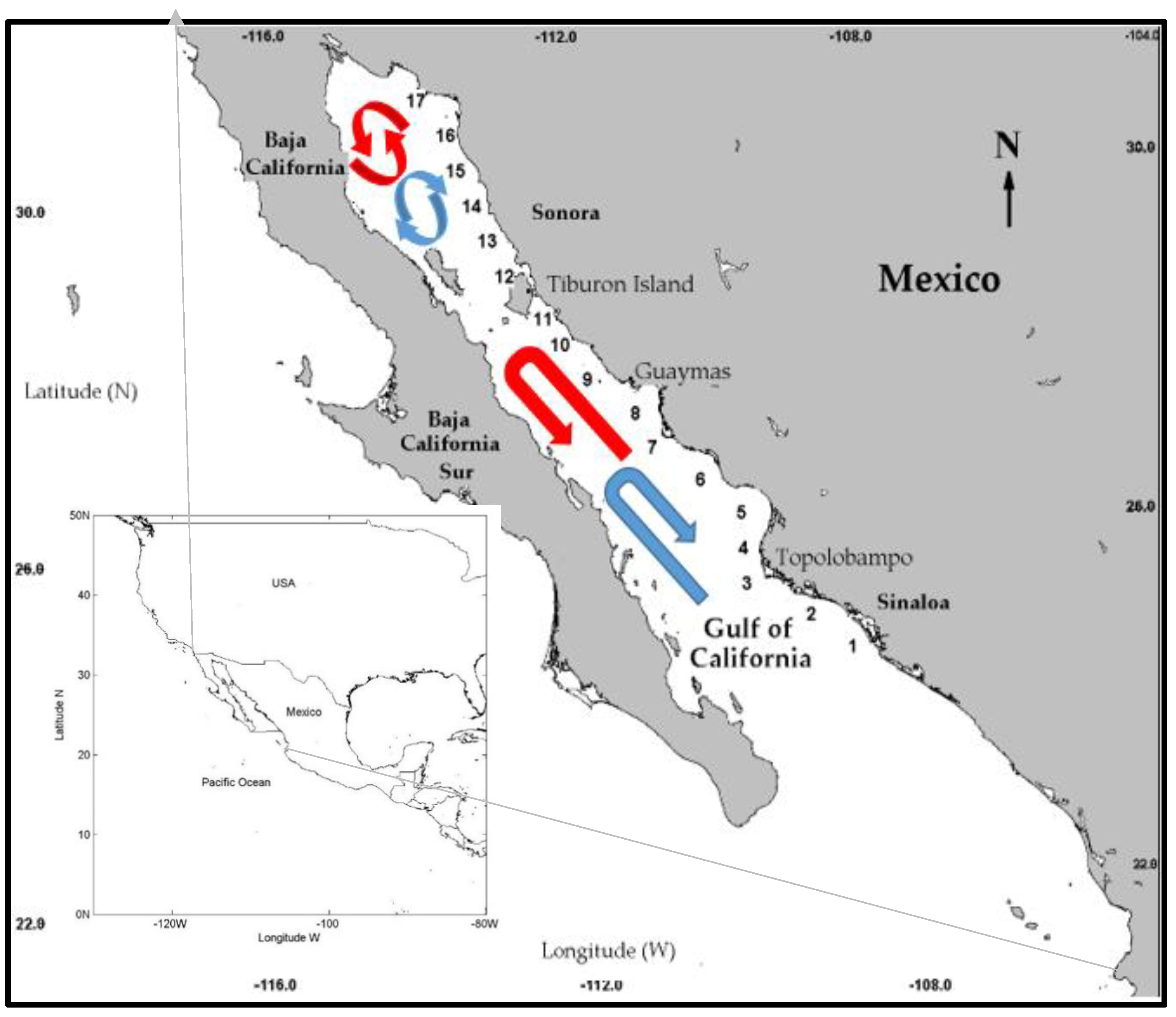
The Gulf of California (GC) is a semi-closed sea situated in the northwest of Mexico; its dimensions are roughly 150–200 km wide and 1100–1400 km long including the entrance zone to the GC with depths varying from about 200 m at the head to 3600 m at the mouth. The general circulation and its seasonal variability result from the forcing of the Pacific Ocean (PO) at its opening (water mass intrusions and tidal motion of low frequency) [5]. The GC is characterised by being a very dynamic sea with tidal currents, seasonal winds, upwelling systems, and high solar radiation; these characteristics determine the strong physical dynamics attributed to mesoscale processes (such as thermocline and surface circulation induced by the wind, gyres, and filaments [6,7]), which develop high productivity levels, nutrient concentrations, and dispersion [8,9].

The gulf shows upwelling processes on the mainland coast with strong northwest winds that cause winter conditions from December to May, and off the Baja California Peninsula coastline with calm southern winds developing summer conditions from July to October where June–November are the transition months between these seasons [7]. During winter conditions, the northwest winds increase the phytoplankton biomass [10] while during the summer conditions, a strong stratification occurs in the water column, and the upwelling processes do not influence the phytoplankton levels [11].

The northwest coastal winds produce surface forcing of the sea in the mainland coast of the GC that goes to the south through the winter–spring months and to the north in the summer–fall months [12]. These oceanographic scenarios in the GC contribute to the development of optimal feeding, breeding, and refuge areas for nektonic species, such as shrimp and sardines, as well as for benthic marine invertebrates. The presence of mixing processes in the subsurface promotes phytoplankton and zooplankton fertilisation inducing optimal habitats and favouring food webs [13].

The GC is also one of the most important marine biodiversity habitats where some of the species are endemic and important for conservation, such as totoaba (Totoaba macdonaldi) and marine vaquita (Phocoena sinus) due to their status as endangered species [14]. Due to the high primary productivity levels, the GC represents an important fishing zone with different types of activities; for example, from highly industrialised pelagic to coastal artisanal fisheries that obtain different products, such as shrimp, small pelagic fish (sardine and anchovy), and squid, as well as large pelagic fish (tuna and marlin) where the catch volumes depend largely on the food availability in the first trophic levels [14,15].

Chlorophyll a (Chl a) plays an important role in studies where the oceanographic variability is of primary interest as the quantification of phytoplankton biomass and its distribution are fundamental to determine primary productivity levels [16,17]. These levels are necessary to analyse the fluctuation of carbon fluxes in the ocean–atmosphere interaction [16,18]. In addition, it is helpful to determine the ocean fertility levels [19], and thus the trophic state index, which has been currently considered of great significance for climate regulation and biochemical cycling [20]. Primary phytoplankton production is the main basis of the pelagic ecosystem trophic web of oceans and aquatic systems; this situation quantifies the conversion rate of carbon dioxide into organic carbon through photosynthesis [21].

However, over the past century, oceanographic analyses have shown a decline of the global Chl a concentration [22,23] generated by climate and oceanographic variability, caused by the increase of the sea surface temperature (SST), stratification augmentation, and, consequently, limited nutrients [22]. Climate changes are modifying biotic and abiotic environments (physical conditions, nutrients, and foraging pressure), which affect the different species, community structures, and phytoplankton population dynamics, impacting the aquatic ecosystems through alterations in the base of the food web and, thus, altering entire ecosystems [20].

The availability of remote sensing measurements with high spatial and temporal resolutions over a wide range of environmental variables allows researchers to obtain reliable data on a greater scale for the physiobiological characteristics of the oceans [24]. Particularly, the large scale satellite observations of ocean colour (Chl a) are crucial for studying tendencies and climate changes [25] in addition to understanding the role of phytoplankton in the biochemical cycles. Moreover, identifying a series of mesoscale phenomena, such as upwelling, mixing, convergence, and dispersion processes (such as oceanic turns) allows researchers to understand their influence on the distribution and abundance of fishing species [26].

Along the GC, high concentration zones of Chl a were found, such as in the midriff islands region (MIR) and the mainland coast with a gradient from the highest to the lowest Chl a concentration from north to south, respectively [27,28]. This variability determines eutrophic conditions in the MIR and mesotrophic or oligotrophic conditions in the southern GC [27]. These conditions are associated with the physical dynamics of tide mixing, seasonal winds, upwelling systems, and stratification [27,29], causing high Chl a concentrations during winter–spring and low concentrations in summer–autumn [27,28,30]. Likewise, Espinosa-Carreón and Valdez-Holguín [31] found a gradient of Chl a from the least to the greatest concentration from south to north in the GC with an annual and interannual variability, related to El Niño-La Niña events.

Herrera-Cervantes et al. [32] reported that El Niño events were non-homogeneous along the GC and more variable in the eastern coast and the northern region of the gulf—represented by a decreasing/increasing pattern of Chl a—while the opposite pattern was observed in the SST, reflecting the strong physical–biological coupling during the El Niño-La Niña events. Another study analysed the effects of the mesoscale phenomena on Chl a concentration in the mainland coast of Sonora and determined that the environmental conditions in the GC were influenced by the seasonal and interannual variability on the meteorological processes and oceanographic dynamics that occurred in it, thus affecting the marine ecosystems [33].

Currently, most of the environmental and oceanographic studies on the GC coast have been only performed in specific regions; for example, due to the low interest in studies along the entire mainland coast with greater coverage, bays and coastal lagoons could provide more environmental information and oceanographic dynamics. Coastal areas are known to be highly vulnerable due to natural variations in the environment and anthropogenic effects; therefore, more information is needed on the environmental and oceanographic conditions and their effects on these coastal areas.

Given the above, long-term observations through remote sensors are important for analyses and the constant monitoring of changes in marine ecosystems and mainland coastal zones; these changes are caused by environmental variability and allow a better understanding of the population dynamics of natural resources—mostly in areas with high temporal and complex spatial fluctuations [34,35], such as the coastal zones of the referred area.

In a previous study, Robles-Tamayo et al. [36] reported a spatial and temporal variation of the SST along the coast of the GC. Their descriptive analysis of SST series showed that the values decreased from south to north, and the amplitude of the warm period decreased from south to north (the cold period increased from south to north). The minimum values occurred during January–February with the maximum values in August–September. Therefore, the objective of this study was to perform a temporal-spatial characterisation of Chl a concentration variability, its effects on the ecosystem in the mainland coastal zone of the GC, and the causes of such variability by analysing satellite images from the Moderate-Resolution Imaging Spectroradiometer Aqua (MODIS-Aqua) sensor.

2. Materials and Methods

2.1. Study Region

This study covers the mainland coast of the Gulf of California (GC), which is characterised by having a great diversity of coastal ecosystems, estuaries, sandy beaches, coastal lagoons, and muddy bays with a wide shelf and supply of fresh water that reaches the coastline through rivers [14]. High fertility levels induced by upwelling effects and river discharges have developed fishing activities in specific ports, such as Guaymas Bay, Yavaros Bay, and Topolobampo Bay. In addition, high irrigation coming from farmlands and aquaculture farms has a bearing on the pigment concentration [37,38]. A seasonal pattern was observed in the pigment concentration, which influences the biological production, obtaining pigment-rich water at the northeast of the mainland side during winter and expanding this high-pigment concentration water to the southwestern region in the peninsular side. However, in summer, water with higher productivity contracts in the opposite direction, remaining a small coastal line that is rich in nutrients [8,12,39]. The sampling coverage sampling points where the Chl a data was obtained went from north Sinaloa State to north Sonora State; these points were georeferenced along the coastal zone, separated approximately 60 km apart from each other and 30 km offshore (Figure 1).

2.2. Environmental Analysis of Chlorophyll a Data

The chlorophyll a data were downloaded in HDF (Hierarchical Data Format) from the OceanColor Web of NASA’s level 3 and are processed from the geophysical parameters that have been placed into a defined grid over a defined time period. The level-3 standard-mapped images (SMI) are representations of binned data products—one for each geophysical parameter stored in each group. Each SMI product represents a data group where the mean is used to obtain the values for each grid, where each SMI product contains one image of the study parameters that can be obtained in different temporal and spatial scales, as well as day or night. [41]. The Ocean Color Web sensor used to obtain the Chl a data was the Moderate-Resolution Imaging Spectroradiometer Aqua (MODIS-Aqua). These measurements were obtained during the period from July 2002 to July 2019, with the purpose of generating an informative database. This sensor corresponded to the chlorophyll concentration using the Ocean Color Index (OCI) Algorithm in milligrams per cubic metre (mg/m³) with a spatial resolution of 9 km.

Additionally, a series of monthly high-resolution images of the Chl a concentration—corresponding to the months of March and August—were used to characterise the greater and lesser seasonal Chl a concentration. These images from 2011 and 2015 were characterised as La Niña and El Niño years, respectively, to graphically represent these two episodes and their effects on Chl a on the GC mainland coast.

This algorithm of Chl a returns the near-surface Chl a concentration in mg/m³, which was calculated using an empirical relationship derived from in situ Chl a measurements and two algorithms of green band ratios. The Chl a product combines two algorithms—the O’Reilly band ratio OCx algorithm and the Hu colour index (CI) algorithm. The CI algorithm is a three-band reflectance difference algorithm, which utilises the difference between the Remote Sensing Reflectance (Rrs) on the green band and a reference formed linearly between the Rrs on the blue and red bands where blue, green, and red are the instrument-specific wavelengths closest to 443, 555, and 670 nm, respectively [42]. The Windows Image Manager software (WIM version 9.06) 1991-2015, Copyright^© Mati Karhu ([email protected]), was used to analyse and obtain the average monthly data of the Chl a images for each sampling point in the years from 2002 to 2019.

2.3. Processing Chlorophyll a Data

For the environmental characterisation of Chl a in the GC, a spatiotemporal analysis was developed through monthly Chl a satellite images from 2002 to 2019, throughout the GC mainland coast in each one of the 17 sampling points that were systematically located. Once the monthly Chl a data of each sampling point were obtained, an analysis of the latitudinal climatology was done through a Hovmöller Diagram with the objective of describing the latitudinal gradient of Chl a concentration along the area during the period of study. In addition, a cluster analysis was performed using the Chl a data for grouping the sampling points with similar characteristics. However, the resulting clusters were not geographically close.

Therefore, for the development of the environmental and oceanographic analyses in the mainland continental coast of the GC, the cluster analysis obtained by Robles-Tamayo et al. [36] was used where four regions were determined with similar environmental characteristics based on the monthly SST data. Once the four regions were determined, the data analysis was performed through an analysis graph of the monthly and annual Chl a variability with time series and annual cycle plots, respectively. A Fast Fourier Transform was performed on these time series to obtain their spectral density and determine the main frequencies of variation (seasonal, semi-annual, annual, and interannual).

The data were transformed to identify anomalies by subtracting from each monthly Chl a value their respective monthly mean and dividing by the standard deviation. The anomalies were smoothed through an exponential smoothing process, making the comparison of the resulting time series easier with the monthly records of the Southern Pacific Oscillation Index (SOI)—downloaded from the National Oceanic and Atmospheric Administration (NOAA)—and also smoothed using the same method. We performed descriptive statistical analyses, including box plots, time series, and annual cycle plots, to analyse the Chl a variability, adding also some time series and annual cycle plots by region.

Certain receiver operating characteristic (ROC)-curves were included to study the Chl a concentration, as this is a statistical tool that permits the identification of differences between two regions based on the monthly mean of the Chl a values; this situation occurs when the Confidence Interval (CI) for the Area Under the Curve (AUC) does not include the 0.5 value [43]. The Kruskal–Wallis test (p < 0.05) was also used [44] to detect statistically significant differences of the Chl a concentration between the four regions. The analyses were performed using different software: Statistica (version 8) 1984–2007, Copyright^© StatSoft, Inc. (www.statsoft.com), R (version 3.6.0) Copyright^© 2019 The R Foundation for Statistical Computing (www.r-proyect.org), and MATLAB (version 9.1.0) Copyright^© 1984–2016 The MathWorks, Inc (www.MathWorks.com). In addition, monthly satellite images of March and August, from 2011 and 2015 (years characterised as La Niña and El Niño events) were used to show the Chl a variability (months and years with different Chl a concentrations) according to the climatological analysis.

3. Results

3.1. Distribution and Variation of Chlorophyll a

The Chl a variation (Figure 2) showed a latitudinal gradient with a general average concentration with values from 0.8 to 3 mg/m³. The major concentrations were observed in 2003 and 2012 with values up to 3 mg/m³ while the low concentrations were observed in 2002–2003 and 2015–2016. Figure 2 shows the south region located between 24° and 26° N latitude and the islands and north region between 28° and 30° N latitude with the lowest values of about 0.8 mg/m³ in 2002–2003 and 2015–2016. In the central area located between 26° and 28° N latitude degrees, the values were observed with a range from 1.5 to 2.3 mg/m³ along the period of study, mainly from 2004 to 2018. The highest Chl a levels were mainly located at the central and northern areas of the gulf with average values that ranged from 2.3 to 3 mg/m³. Regarding the lowest values, they occurred at the south and north GC with a minimum average concentration of about 0.8 mg/m³.

3.2. Cluster Analysis

The conglomerate analysis gathered the Chl a values in four clusters when the linkage distance units were greater than ten (Figure 3). When this figure is analysed from left to right, the first and fourth groups include the sampling points two and one, corresponding to the south region (SR). The tenth and eleventh sampling points constitute the second cluster midriff islands region (MIR) while the third cluster includes the remaining sampling points, mostly from the central and north regions (CR and NR), respectively. The resulting clusters were not geographically close due to diverse factors that shall be explained in the discussion section. Therefore, from now on, the SST cluster that classified the four regions obtained by Robles-Tamayo et al. [36] shall be used for the Chl a analyses.

3.3. Annual Cycle Variation and Climatology

The time series analyses for the Chl a monthly data for each region showed values ranging from 0.2 to 8 mg/m³. Chl a values in the SR (Figure 4) ranged from 0.2 to 6 mg/m³ while it ranged from 0.2 to 5 mg/m³ in the CR, and the variability was small (Figure 5). The MIR (Figure 6) showed the widest values of Chl a (0.4–8 mg/m³) whereas the NR (Figure 7) showed the narrowest ones (0.2–4 mg/m³). The SR and MIR showed high levels in the Chl a concentration from 2002 to 2012 with values up to 6 and 7 mg/m³, respectively; after that year, the Chl a levels recorded an important decrease with values close to 4 mg/m³ from 2013 to 2016. This effect was not significant in the CR, particularly in the NR where the Chl a levels did not show much variability.

Overall, a range approximately from –0.9 to 1.4 units was observed for all Chl a anomalies. In the SR (Figure 8), they varied from –0.86 to 1.28 units, while in the CR (Figure 9), the range was from –0.64 to 1.32 units. The MIR (Figure 10) showed a range from –0.67 to 0.92 units while anomalies varied from –0.62 to 0.78 (Figure 11) in the NR. The widest range of Chl a anomalies occurred at the CR and the narrowest ones were at the NR. We compared the Chl a anomalies for each of these regions with those in the database of the SOI index, which ranged from –0.93 to 1.45 units. The negative values of the SOI index coincided with warm waters related to El Niño events, while positive values concurred with cold waters associated with La Niña events. These interannual events caused an effect in Chl a variability with a similar behaviour than the ones described previously. In addition, a delayed response of the Chl a concentration was observed with the SOI index in 2009 and 2015, characterised as Niño years (moderate and very strong, respectively).

Analyses of the monthly Chl a data for each one of the regions (

Table 1. Descriptive statistics of the chlorophyll a (Chl a) concentration on the mainland coast of the Gulf of California (GC).

Region	Mean ± SD (mg/m3)	Max (mg/m3)	Min (mg/m3)
South	1.31 ± 1.20	6.12	0.24
Central	1.19 ± 0.87	4.29	0.22
Midriff Islands	2.12 ± 1.43	7.42	0.49
North	1.20 ± 0.68	3.44	0.29

). The highest Chl a mean concentration occurred in the MIR while the lowest was in the CR. Regarding the Chl a variability, the lowest occurred in the NR, whereas MIR had the greatest variability.

The climatology of the Chl a concentration over the year showed a seasonal variation in all the regions, reaching the maximum values in March, decreasing later until they reached the minimum values from July to August, and rising again from October to November (Figure 12). The SR had a maximum of 2.88 mg/m³ and minimum of 0.37 mg/m³ while the CR reached its maximum at 2.55 mg/m³ and a minimum of 0.31 mg/m³. The MIR showed the highest Chl a concentration with a maximum of 4.35 mg/m³, and its minimum was 0.77 mg/m³, whereas the NR had a maximum of 2.32 mg/m³ and a minimum of 0.41 mg/m³. The climatology of each one of the regions had similar behaviour with the general climatology obtained for the mainland coast of the GC. This showed a seasonal variability with the maximum values in March (2.6 mg/m³), decreasing later with the minimum values in August (0.4 mg/m³), and increasing again in October, reaching a concentration of 1.5 mg/m³ in November. This Chl a seasonal variability is characterised with “winter” and “summer conditions” of the GC, respectively.

The monthly images of Chl a of March and August of 2011 and 2015 were taken to show the Chl a distribution according to the results of the climatology analysis (months with greater and lesser concentration of Chl a, respectively) and the Hovmöller Diagram (years characterised as La Niña and El Niño, respectively) (Figure 13).

Robles-Tamayo et al. [36] identified two periods when they analysed monthly the SST data: a warm period (WP) where the SST values were higher than 25 °C, and a cold period (CP) where these values were lower than 25 °C, with transition periods around this temperature from May to June (warm) and November (cold). These periods were used in this study to make the statistical description of the Chl a concentration (

Table 2. Statistical analysis of chlorophyll a (Chl a) concentration on the mainland coast of the Gulf of California (GC) warm period (WP).

Region	Time (months)	Mean ± SD (mg/m3)	Max(mg/m3)	Min (mg/m3)
South	7	0.79 ± 0.89	6.04	0.24
Central	6	0.55 ± 0.37	2.18	0.22
Midriff Islands	5	1.19 ± 0.83	5.52	0.49
North	4	0.63 ± 0.39	2.73	0.29

and

Table 3. Statistical analysis of chlorophyll a (Chl a) concentration on the mainland coast of the Gulf of California (GC) cold period (CP).

Region	Time (months)	Mean ± SD (mg/m3)	Max (mg/m3)	Min (mg/m3)
South	5	2.05 ± 1.20	6.12	0.47
Central	6	1.84 ± 0.73	4.29	0.74
Midriff Islands	7	2.80 ± 1.40	7.42	1.03
North	8	1.50 ± 0.61	3.44	0.53

). During both periods, the mean Chl a values were higher in the SR and the MIR and lower in the CR and NR.

Box and Whisker plots were performed for comparing the monthly Chl a concentration in each one of the regions (within each period) observing clear differences in their location and variability (Figure 14). The lowest values of the Chl a concentration were observed during the WP and the greatest ones in the CP; whereas, the Chl a variability was greater at the MIR and the SR.

On the other hand, the ROC curves allowed us to compare the monthly Chl a values among regions within a specific period. The SR and MIR were distinguishable with a CI for the AUC of 0.732–0.856 during the WP (Figure 15). This difference was also observed during the CP, with an AUC CI of 0.591–0.746 (Figure 16), where it was clear that the 0.5 was not in the CI, obtaining different Chl a concentrations in these regions during both periods. These differences were also obtained when the MIR and the NR were compared for both periods, resulting in an AUC CI of (0.786, 0.915) for the WP (Figure 17), while, in the CP (Figure 18), the AUC CI was 0.776–0.876. However, the comparison of the Chl a concentration between SR and NR during the WP was not significant (Figure 19), not rejecting the hypothesis of similar Chl a levels in that period between those regions. ROC-curve statistics including the cut-off, specificity, sensitivity, AUC, and AUC CI are described in

Table 4. ROC-curve summary statistics for the chlorophyll a (Chl a) concentration on the mainland coast of the Gulf of California (GC) warm period (WP). (*) indicates significant differences (0.5 is not in the area under the curve (AUC) colour index (CI).

Regions	Cut-off	Specificity	Sensitivity	AUC	AUC CI
SR-CR	0.375	0.750	0.447	0.594	0.519–0.669*
SR-MIR	0.615	0.667	0.907	0.794	0.732–0.856*
SR-NR	0.365	0.233	0.971	0.541	0.460–0.622
CR-MIR	0.575	0.699	0.942	0.870	0.819–0.921*
CR-NR	0.385	0.476	0.913	0.644	0.562–0.726*
MIR-NR	0.565	0.953	0.652	0.850	0.786–0.915*

and

Table 5. ROC-curve summary statistics for the chlorophyll a (Chl a) concentration on the mainland coast of the Gulf of California (GC) cold period (CP). (*) indicates significant differences (0.5 is not in the area under the curve (AUC) colour index (CI).

Regions	Cut-off	Specificity	Sensitivity	AUC	AUC CI
SR-CR	2.665	0.329	0.882	0.508	0.419–0.598*
SR-MIR	1.435	0.435	0.874	0.669	0.591–0.746*
SR-NR	2.145	0.435	0.860	0.608	0.523–0.692*
CR-MIR	2.305	0.784	0.563	0.724	0.658–0.789*
CR-NR	1.285	0.794	0.478	0.651	0.581–0.721*
MIR-NR	1.695	0.782	0.713	0.826	0.776–0.876*

for the WP and CP, respectively.

We performed a comparison of the monthly Chl a concentration for all the regions during each one of the periods using the Kruskal–Wallis test. As significant differences were observed (p < 0.00001), the Bonferroni multiple comparison post hoc test was used to detect them. The results of this test are shown in

Table 6. The Bonferroni 2-tailed p-values for the monthly chlorophyll a (Chl a) concentration multiple comparison between regions during the warm period (WP) on the mainland coast of the Gulf of California (GC). (*) indicates significant differences.

Regions	South	Central	Midriff Islands	North
SR		0.06170	0.00022*	0.77932
CR	0.06170		2.6E–09*	1.00000
MIR	0.00022*	2.6E–09*		3.8E–06*
NR	0.77932	1.00000	3.8E–06*

and

Table 7. The Bonferroni 2-tailed p values for the monthly chlorophyll a (Chl a) concentration multiple comparison among regions during the cold period (CP) on the mainland coast of the Gulf of California (GC). (*) indicates significant differences.

Regions	South	Central	Midriff Islands	North
SR		0.89888	2.8E-06*	0.00054*
CR	0.89888		7.7E–11*	0.06572
MIR	2.8E–06*	7.7E–11*		<2E–16*
NR	0.00054*	0.06572	<2E–16*

, where the significant p-values are denoted with an asterisk (*). During the WP, the Chl a concentration in the MIR was statistically different from all the others, while in the CP, no differences were found either between the SR and CR or the CR and the NR.

3.4. Spectral Analyses

The Chl a variability through the Fourier analyses in all the regions (Figure 20, Figure 21, Figure 22 and Figure 23) determined the annual frequency as the primary one, followed by the semi-annual, seasonal, and inter-annual. The Fourier analyses also showed a rise of the semi-annual frequency from the south to MIR and a decrease in the NR. Regarding the seasonal frequency, which was observed in all the regions, an increase from the SR-MIR occurred with spectral densities similar to the ones observed in the semi-annual frequencies of the CR. In the SR and MIR, the interannual frequencies were higher than the ones observed at the CR and NR. Based on these results, a major influence of the El Niño phenomenon was observed in the SR and MIR. The same results were corroborated with the Hovmöller Diagram (Figure 2).

4. Discussion

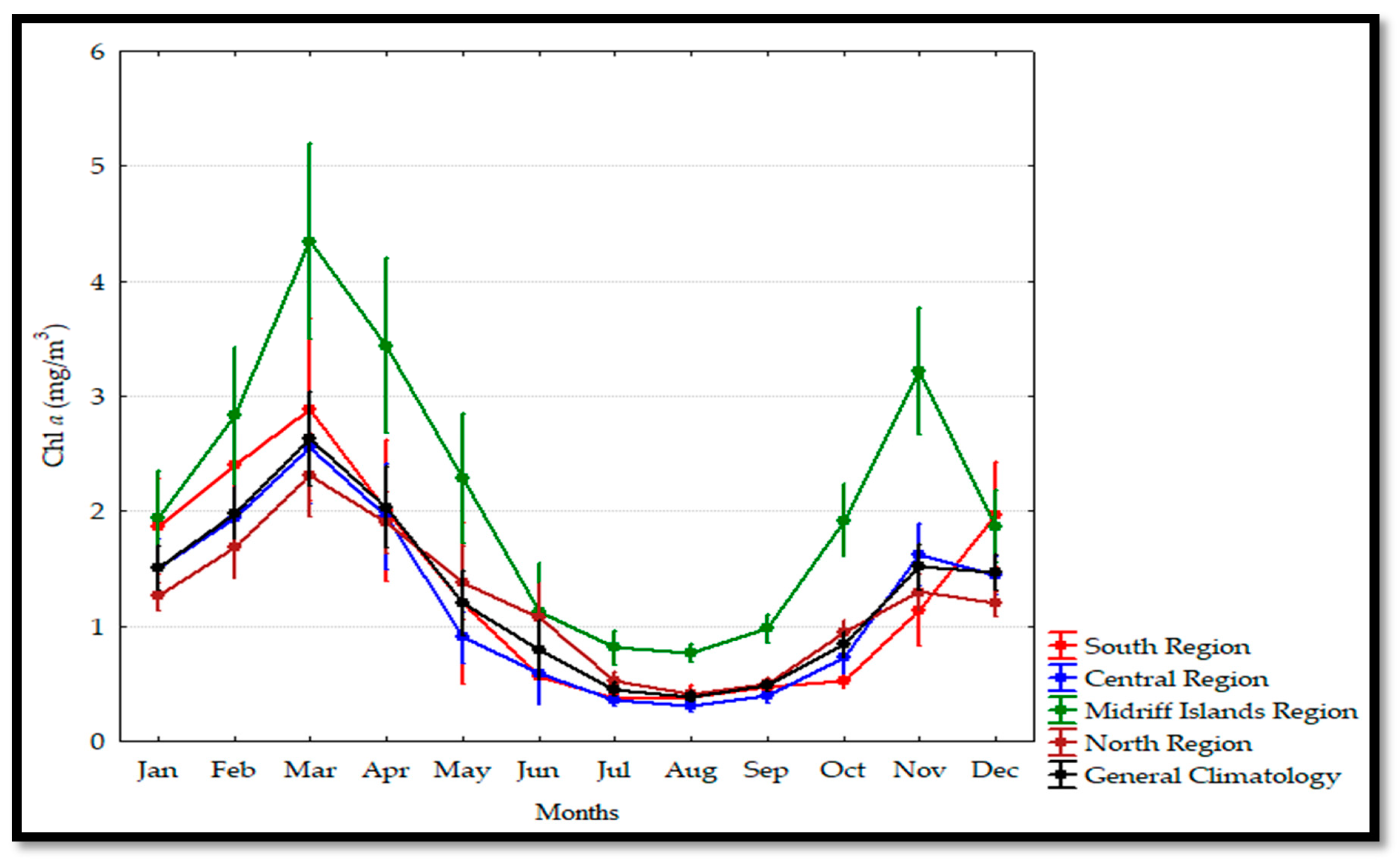
The Chl a climatology analysis of the Gulf of California mainland coast showed clear latitudinal differences associated with atmospheric circulation, such as seasonal wind patterns [6,7,45] that have an influence on the gulf circulation and consequently on oceanographic variables, such as the chlorophyll a concentration. In this study, the general climatology showed a seasonal variability with the maximum values in March and minimum values in August. The variability can be explained by the three main fertility systems that occur in the GC (upwelling, tide mixing, and water exchange with the Pacific Ocean) that are observed in different areas of the gulf [9], mainly on the eastern coast, which is an area characterised by having upwelling systems that develop high Chl a concentrations up to 10 mg/m³ [9,10].

This general climatology was also reported by García-Morales et al. [33] who found an increment in the Chl a concentration from November to April with the maximum values in March, decreasing from May to October and observing the minimum values from August to September. During the winter, the effects of the winds generated this climatology [7,10,33] as the combination of high-level nutrients, water transportation, and cyclonic gyres caused a dispersion of the total matter in suspension along the coastal zones, having a bearing on the phytoplankton and consequently on the Chl a concentration.

Regional and ecological characterisation have been described using four clusters, previously identified by Robles-Tamayo et al. [36]. Many authors have characterised the GC considering different methods and variables, for example, based on phytoplankton remains in sediments in the water column [46]; time series Chl a analyses all over the gulf for eight years using weekly data [10]; Chl a concentration studies in the cold season [47]; and monthly SST and Chl a data analyses for 18 years [48]. Nevertheless, the results shown in this study have some differences from the ones reported by Hidalgo-González and Álvarez-Borrego [47] who determined four regions along the gulf and a clear seasonal variability as a common result.

With respect to the number of bioregions that the cluster analysis on the Chl a concentration generated, the results are different from those reported by Santamaría-del Angel et al. [10], who classified 14 regions in all the gulf that derived from the weekly Chl a data. Chl a values are more variable than SST values. The physical ocean dynamics (water masses, upwelling systems, and variables, such as temperature and wind patterns generate different phytoplankton concentrations) in the coastal zone are considered a more dynamic area than the open ocean. These factors explain the results obtained in the cluster analysis where the resulting clusters contained sampling points that were not geographically close. Therefore, all the analyses described in this study considered the clusters found by Robles-Tamayo et al. [36], which were based on SST values.

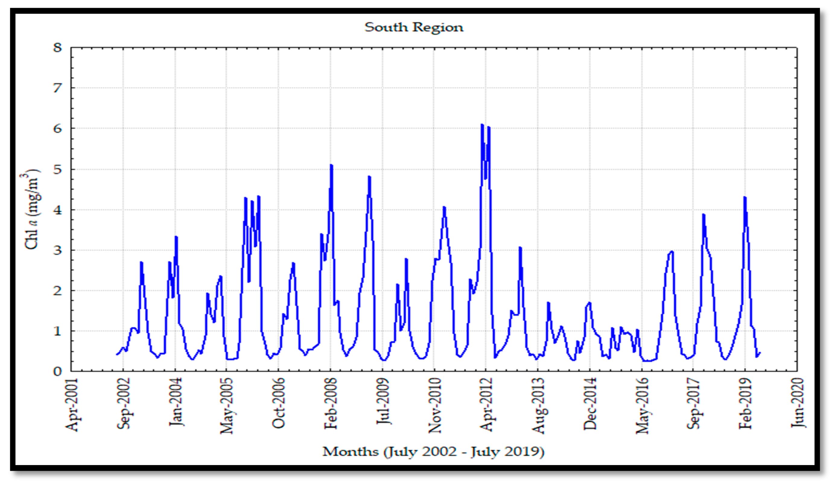
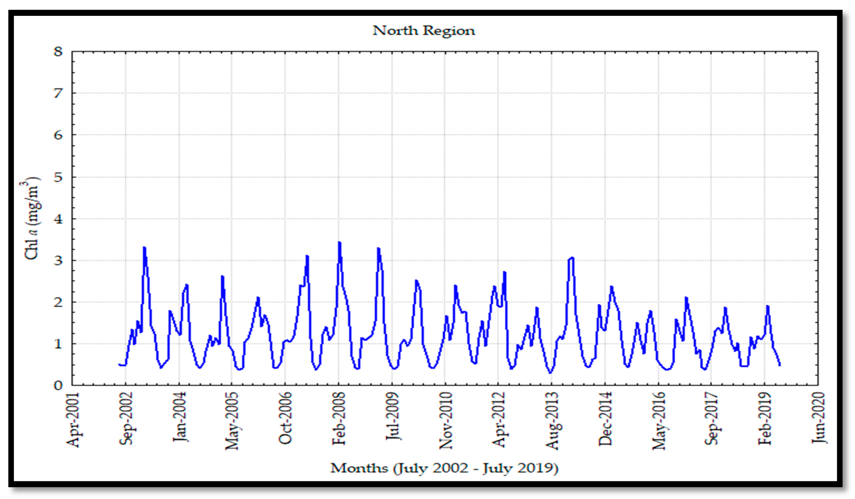
The mean values of the Chl a concentration have a decreasing gradient from SR to NR, except for the MIR where the highest Chl a concentration was observed. The SR showed a high level of Chl a, despite its connection with the Tropical Pacific Ocean that allows the entrance of oligotrophic water, which is warmer than that of the GC [49]. These Chl a values occurred in spite of the high solar irradiance and evaporation effects [45] that generate low chlorophyll concentrations, which can be explained as large farmland runoffs (rich in nitrogen and other elements, such as iron and phosphorus) feed big phytoplankton blooms up to 80% more than in its natural form [38].

Martínez-López et al. [50] reported high levels of chlorophyll in the Lagoon System of San Ignacio Navachiste-Macapule, in the north of Sinaloa State, obtaining concentrations of 15 mg/m³. These high levels are associated with farmland runoffs, seasonal rains, and wastewater effluents, all contributing to the distribution of phytoplankton species and cyanobacteria, which explains the relationship between phytoplankton and the external nutrient contribution. Currently, in the southern coastal zone of Sonora State, high Chl a levels have been also observed, which could be associated with the shrimp farm effluents, as reported by Miranda et al. [51]. This situation indicates that shrimp farm runoff can generate an increment in nutrient quantity, mainly in nitrogen and phosphorus, and thus enhance the level of nutrients in the coastal waters of the GC.

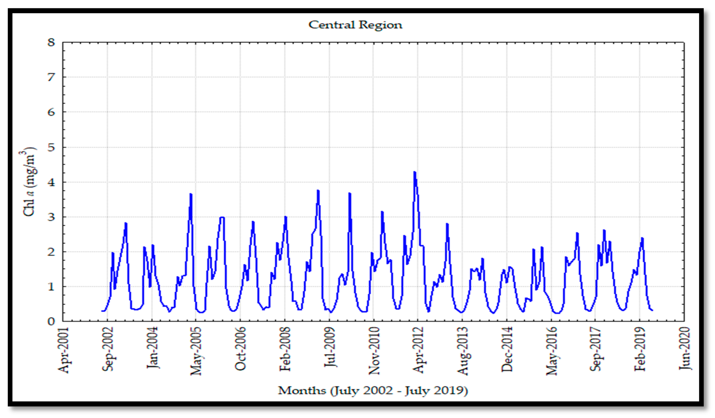
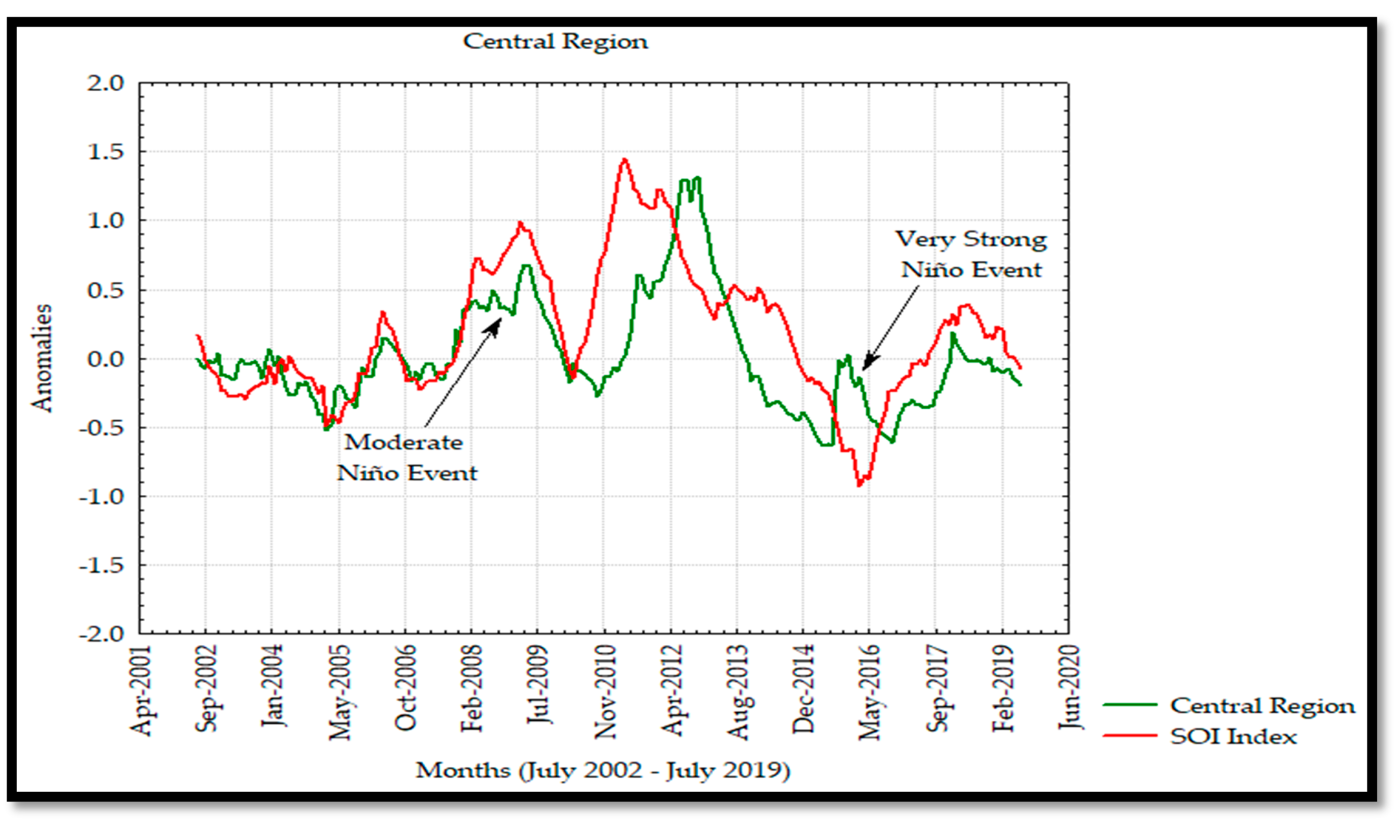
Regarding the central region, the mean values of the Chl a concentration were lower than those observed in the south region. These results were different from the ones reported by Hidalgo-González and Álvarez-Borrego [47], who observed a rise from south to north during the cold season and a slight tendency to rise in the warm season. Lara-Lara et al. [19] found high Chl a levels in the central area of the GC, mainly due to physical dynamics that induced the abundance of phytoplankton. This effect did not occur in other regions of GC, such as in Guaymas Bay where the presence of a greater zooplankton abundance—mainly copepods—generated a major grazing process, affecting Chl a levels that depended on phytoplankton abundance.

Santamaría-del Ángel et al. [10] classified the central area as one with high chlorophyll concentrations, mainly due to the fluctuations of non-simultaneous upwelling events during the spring transition and neap tides. 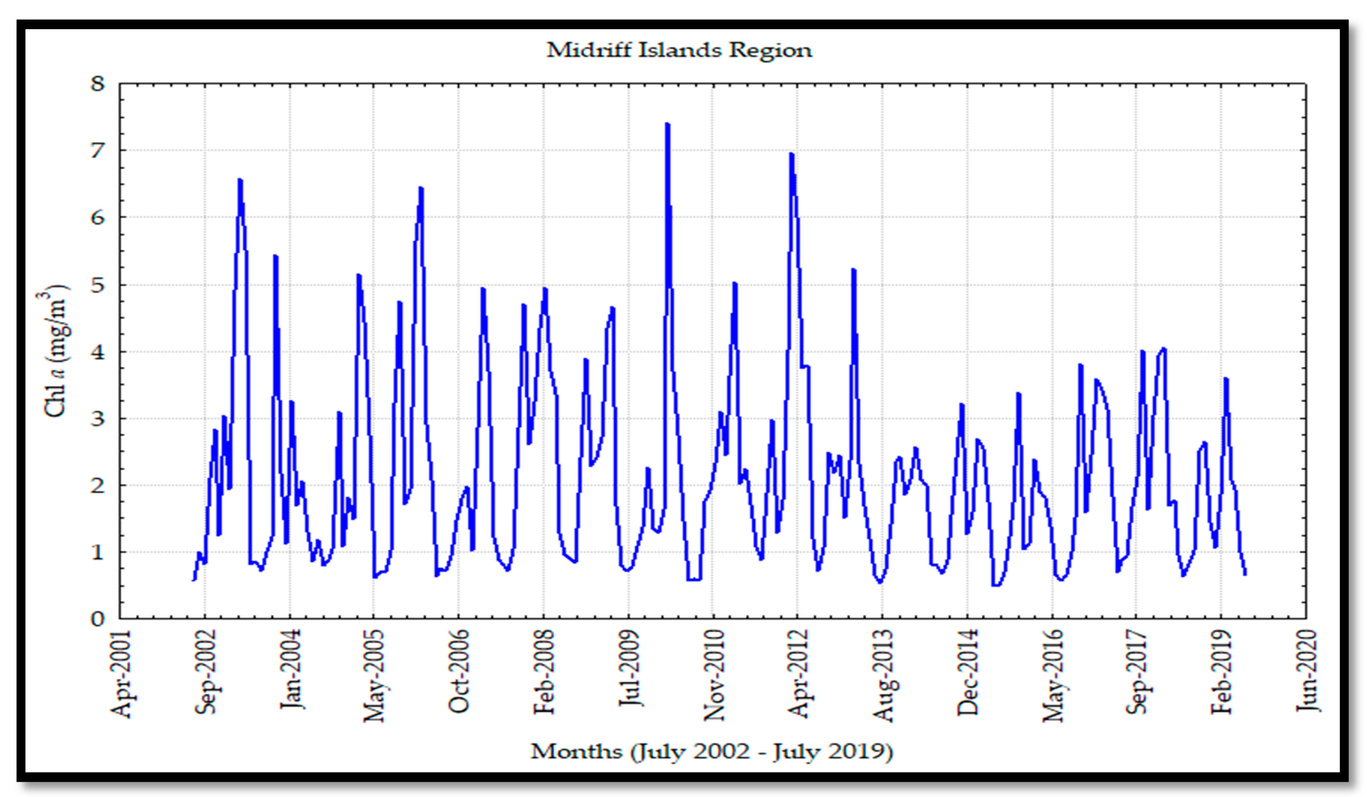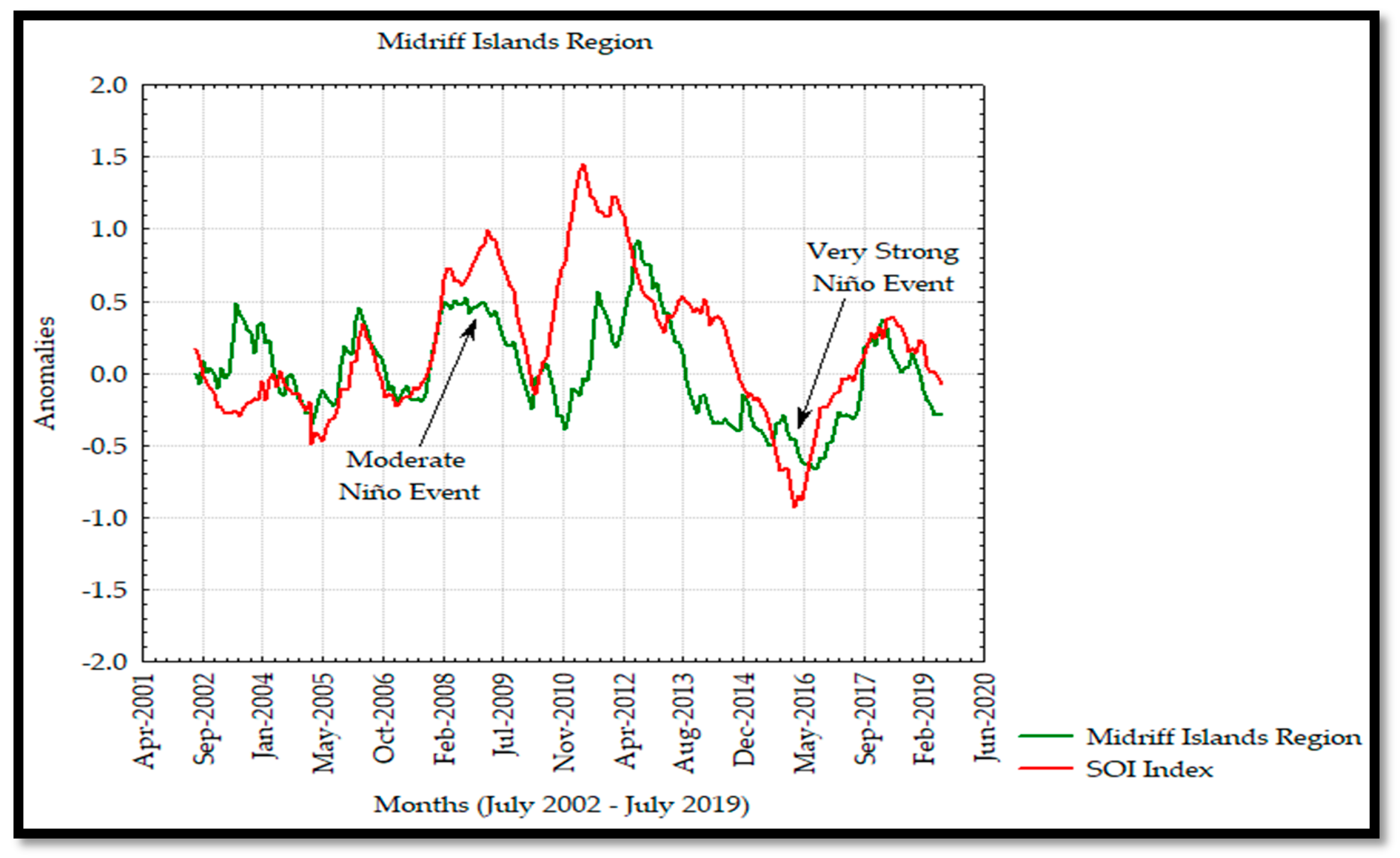Chlorophyll concentration in this region may also be associated with the biological response to the physical dynamics that developed changes in the phytoplankton population structure (the prevailing species capable of acquiring and assimilating low nutrient quantity in oligotrophic waters) [18]. The midriff islands region showed the highest Chl a mean value concentration of the coastal zone, which coincided with the results observed by Hidalgo-González and Álvarez-Borrego [47] and Escalante et al. [28].

These values were associated with tidal mixing (intense wind periods that induce upwelling processes on the mainland coast) [12,29], developing intense currents on the coast of Sonora State, where the El Infiernillo Channel is located. This narrow and shallow channel allowed a well-mixed water column [52], which generated a high nutrient concentration and, consequently, high Chl a levels, in addition to high primary productivity. Santamaría-del Angel et al. [10] also reported that this Chl a concentration was associated with areas with a high upwelling effect and also a high concentration of photosynthetic pigments. The Chl a values in the north region were similar to the ones observed in the central region, which happened despite being an area where high concentrations of nutrients exist by the occurrence of upwelling effects and tidal mixing processes [6,10,30] in a very shallow area (<30 m) [5]; in combination with turbulence, inorganic nutrients, terrigenous types, and total matter in suspension, high turbidity levels were developed.

Lechuga-Deveze et al. [53] reported this effect in Ensenada de La Paz, describing this area as an ideal site of a “trap” of terrigenous sediment, which causes a rise in turbidity, so no light availability exists for phytoplankton, limiting its biomass. Regarding the decreasing–increasing behaviour of Chl a anomalies, this can be explained due to El Niño-Southern Oscillation ENSO events. Herrera-Cervantes et al. [32] also reported some anomaly effects that had an influence on the physical processes associated with the interruption of winds that develop the upwelling effects along the East Coast. With respect to the new primary productivity along the GC, Kahru et al. [54] observed a decrease of about 30%–40% from south to north.

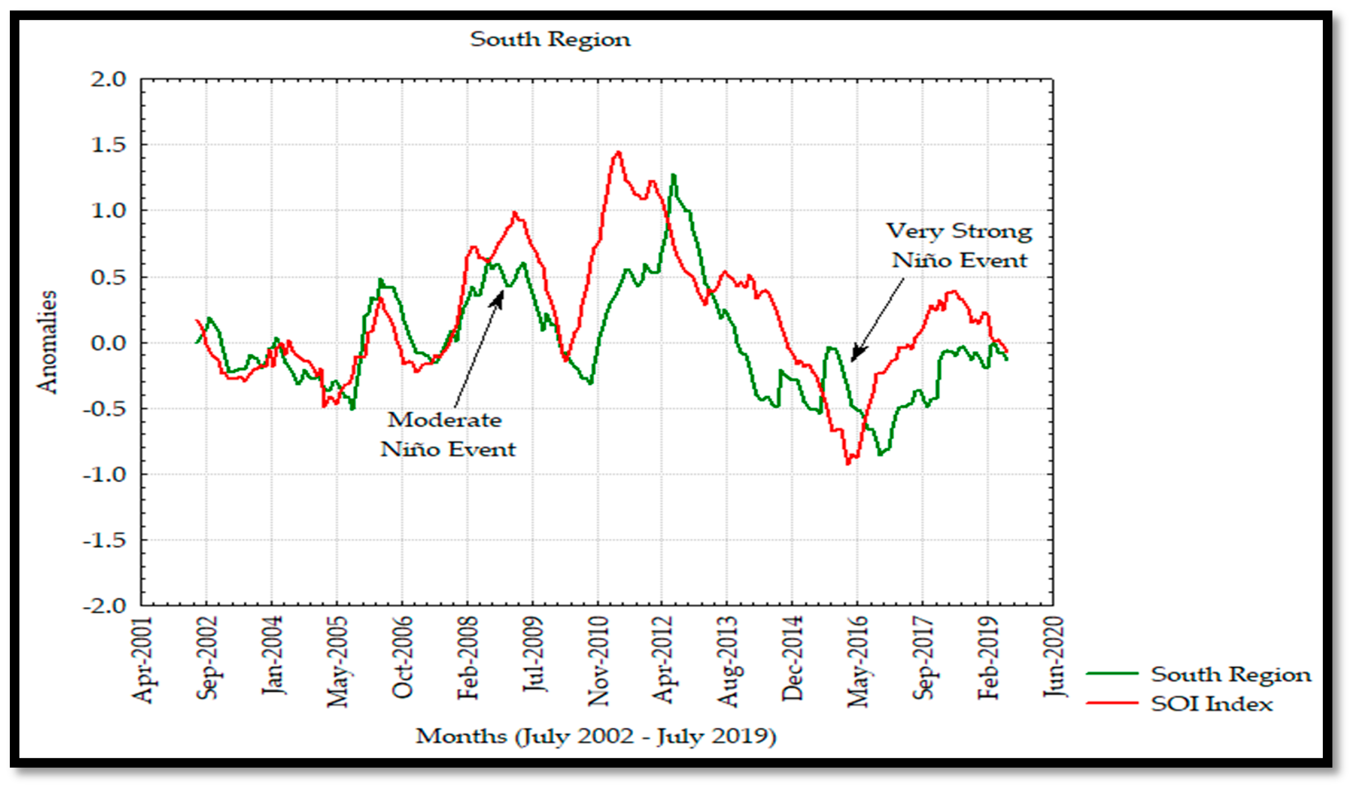
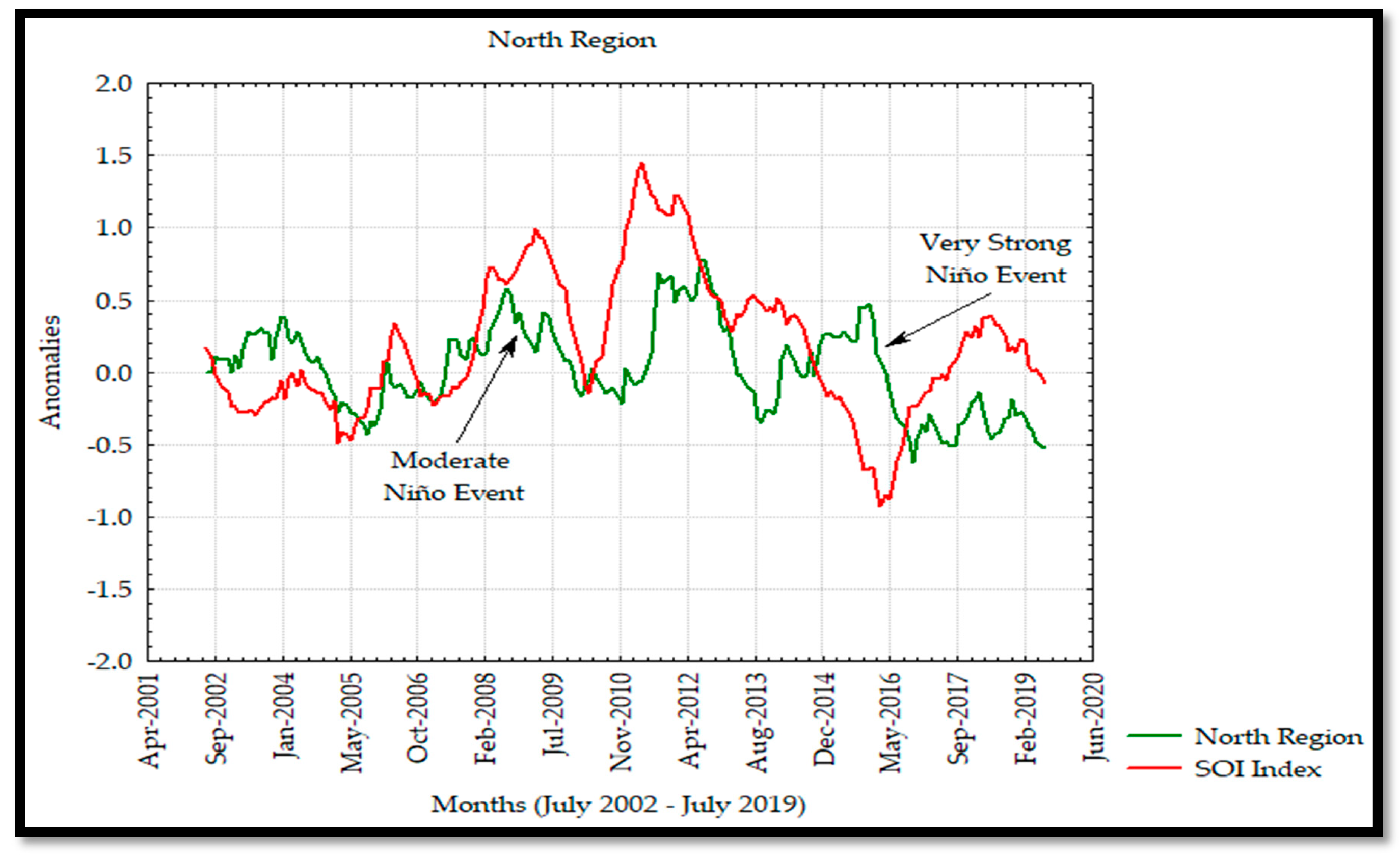
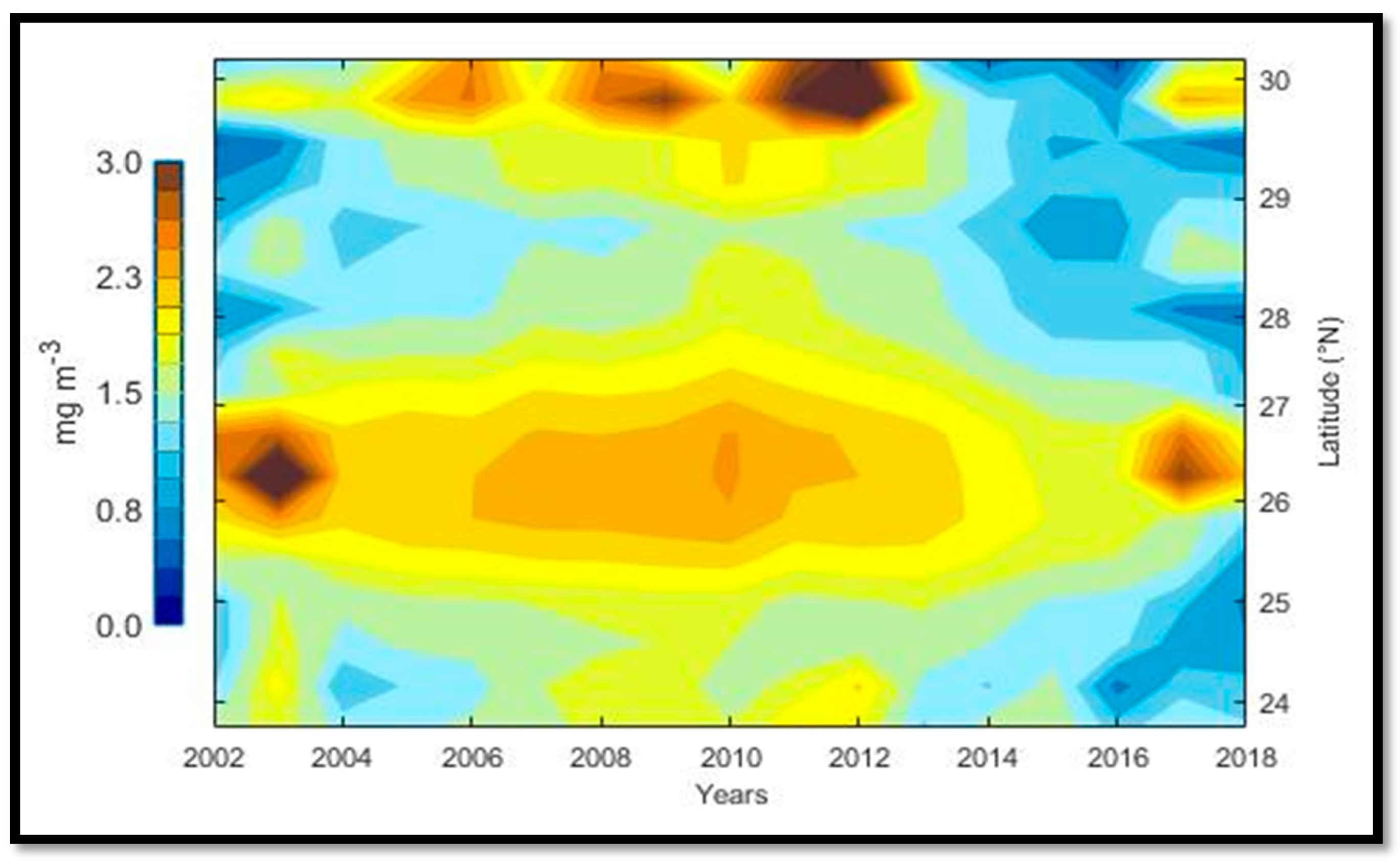
The anomaly analyses shown in this study were similar to those observed by Escalante et al. [28] in the GC where negative and positive anomalies were associated to the interannual La Niña and El Niño events as seen in the Hovmöller Diagram and Figure 13 for Chl a in 2011 and 2015 with negative and positive anomalies, respectively. In addition, the effects of El Niño 2009–2010 and 2015–2016 events were observed to have a significant effect on the Chl a annual variability and causing a decrease in its concentration during these events. On the other hand, the SOI index and Chl a time series showed a strong correlation from 2002 to 2009, and a delayed response was observed from 2010 to 2019, developing a not strong correlation between both time series associated with the moderate El Niño events during 2009 persisting in 2019 due to the very strong El Niño in 2015 [30,55].

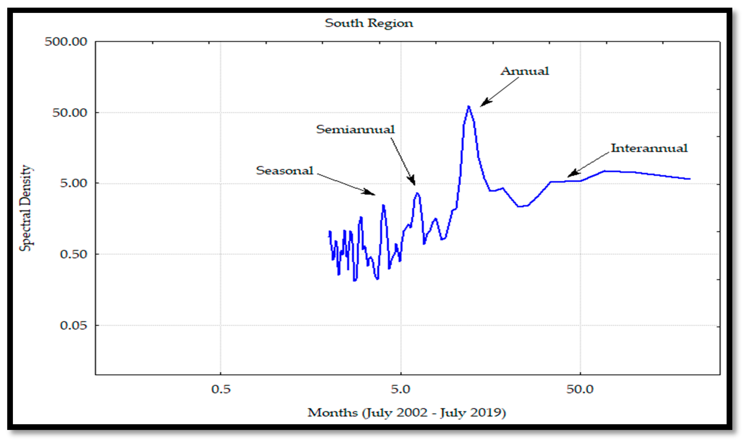
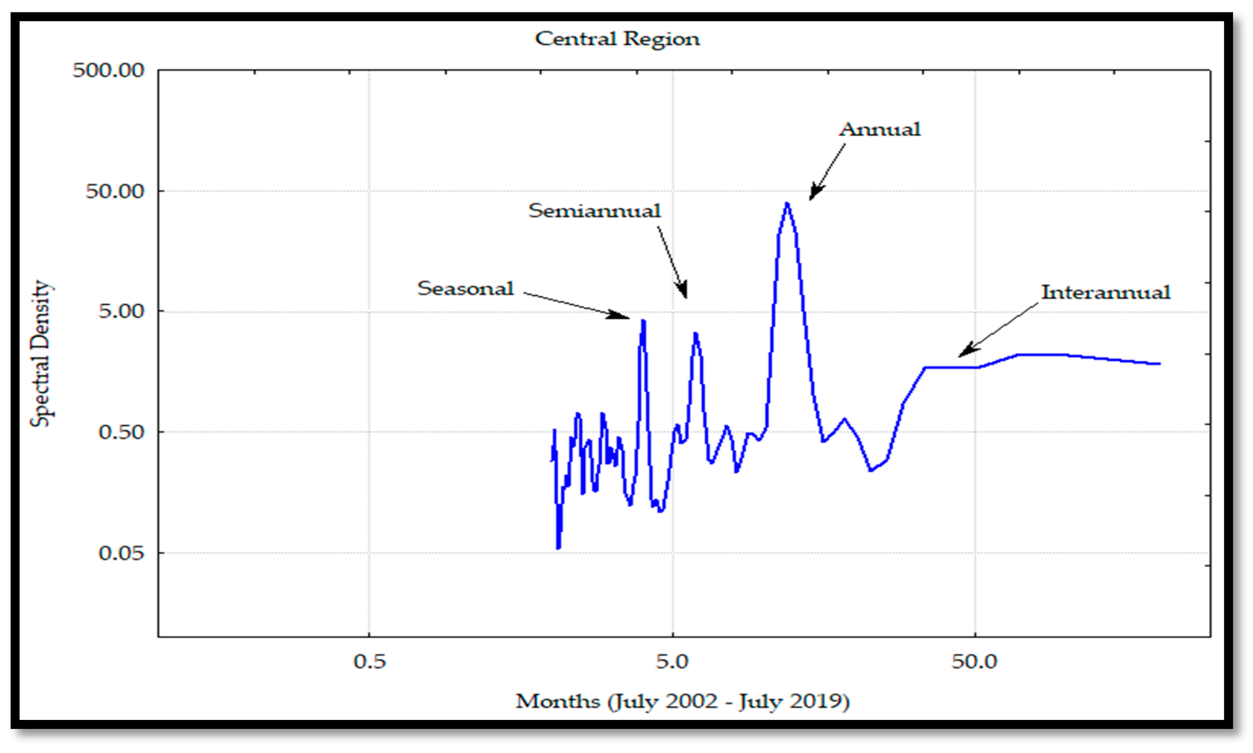
For all the regions, the main frequency was the annual one, as was also reported by García-Morales et al. [33], in conjunction with semi-annual and interannual components. These results were caused by the atmosphere–Pacific Ocean interaction where the seasonal winds developed upwelling effects and cyclonic and anticyclonic gyres [33]; these processes dispersed Chl a, contributing to the nutrient availability and influencing the phytoplankton communities.

In addition, García-Morales et al. [33] explained that the mesoscale phenomena were modulated in three time scales: the seasonal current systems associated with the California current and the Mexican coastal zone, the oceanic gyre effects in the south of the gulf, and the variability observed between years that can affect the marine ecosystems. The semi-annual frequency was determined by the physical dynamics of the zones, as was reported by Álvarez-Molina et al. [29]. These authors explained that the annual and semi-annual variations were due to water circulation changes among the regions, caused by eddies and upwelling effects with high Chl a levels in the CP, and low levels during the WP. This variability was greater in the midriff islands region due to the exchange of cyclonic and anticyclonic circulations during the summer and winter, respectively, which developed a more considerable mixing effect [54].

Kahru et al. [54] also reported that the annual cycle was dominant in the phytoplankton biomass variability, except for the south region and islands regions, where the semi-annual frequency mainly determined this variability. At the central region, the seasonal frequency was larger and easier to identify than the semi-annual one, possibly due to the high gyre circulation pattern [5], which may have an important effect on the seasonal cycle that develops the water exchange at the entrance of the GC. The seasonal pattern is influenced by the coastal upwellings that are determined by the wind intensity in the different seasons of the year and the depth and heterogeneity of the coastline [8]. This situation occurs during the winter and spring on the coasts of Sonora and Sinaloa [12], all generating a rise of the phytoplankton concentration along the coasts.

The interannual frequency was greater in the south and midriff islands regions. This variability was associated with the macroscale oceanic and atmospheric circulation of the PO due to the coupling of this circulation with the El Niño phenomenon. Due to the lack of Chl a data of the mainland coast of the GC, it was not possible to observe the influence of other variability indicators, such as the Pacific Decadal Oscillation (PDO) [15,32], which is associated with El Niño and La Niña events. Espinosa-Carreón and Valdez-Holguín [31] also reported this frequency and found clear evidence of the interannual variability in the Chl a distribution, produced by the El Niño and La Niña events, which caused positive and negative anomalies, respectively, during specific years.

The Chl a variability analysis indicated that mainly physical and climatological processes had an influence on this variable at different spatiotemporal scales; this variability can affect not only the coastal ecosystems but also distribution and abundance of marine resources. Espinosa-Carreón and Valdez-Holguín [31] concluded that the analysis of the seasonal and interannual Chl a variability was important to estimate the fishing potential at a certain time and place. García-Morales et al. [33] concluded that the SST and Chl a variation in the mainland coast of the GC affected the number of species in the marine ecosystem, as well as different species of commercial importance.

Salvadeo et al. [56] analysed the sighting records of Bryde’s whales and environmental variability. They identified that changes in the occurrence of Bryde’s whales were related to the interannual variability in the SST and Chl a in La Paz Bay. The largest number of whales occurred during La Niña conditions, and the fewest were recorded during El Niño events. On the other hand, González-Máynes et al. [57] analysed the jumbo squid (Dosidicus gigas) distribution and abundance and its relation to environmental factors through the SST and Chl a analyses, as well as catch-per-unit-effort (CPUE) of the Pacific sardine (Sardinops sagax) in the central GC. They found that the maximum levels of jumbo squid were obtained at the highest SST values and mean values for CPUE. They also concluded that a non-linear relationship was observed between the environmental-biological parameters and jumbo squid distribution in the Gulf of California. According to the results obtained in this study, it is evident that the Chl a concentration analysis and its constant monitoring were important to obtain updated climatological information for different coastal regions, which could affect diverse ecosystems and possibly influence marine resources.

5. Conclusions

We observed a latitudinal gradient of the Chl a concentration with an evident distribution pattern along the coastal zone. A clear seasonal variability between months in the Chl a analysis was observed with high levels in the spring and low levels in the summer. The comparison of Chl a mean concentrations among regions—during warm and cold periods—produced significant results in many of them. The climatology in the four mainland coast regions of the Gulf of California demonstrated similar behaviours with the maximum values in March and the minimum values from July to August. The largest values were observed in the MIR.

In all the study regions, the main frequency was the annual variability and those associated with the semi-annual, seasonal, and interannual periods. A clear relationship of the SOI index was observed in the first years of this study, contrary to the period from 2010 to 2019 where we observed a clear effect of the 2009–2010 El Niño index (moderate) and 2015–2016 index (strong) in the Chl a annual concentration variability throughout the study area. These effects on Chl caused a delay in the Chl a increase and a lag of Chl a with the SOI index.