Article

Recovery of Rapid Water Mass Changes (RWMC) by Kalman Filtering of GRACE Observations

1
Centre National de la Recherche Scientifique (CNRS), Géosciences Environnement Toulouse (GET), Observatoire Midi-Pyrénées (OMP), 31400 Toulouse, France
2
Université Paul Sabatier (UPS), Géosciences Environnement Toulouse (GET), Observatoire Midi-Pyrénées (OMP), 31400 Toulouse, France
3
Institute of Physics and Meteorology, Computational Science Lab (CSL), University of Hohenheim, 70593 Stuttgart, Germany
*
Author to whom correspondence should be addressed.
Remote Sens. 2020, 12(8), 1299; https://doi.org/10.3390/rs12081299
Submission received: 28 March 2020 / Revised: 15 April 2020 / Accepted: 17 April 2020 / Published: 20 April 2020
(This article belongs to the Special Issue GRACE Satellite Gravimetry for Geosciences)

Abstract

:
We demonstrate a new approach to recover water mass changes from GRACE satellite data at a daily temporal resolution. Such a product can be beneficial in monitoring extreme weather events that last a few days and are missing by conventional monthly GRACE data. The determination of the distribution of these water mass sources over networks of juxtaposed triangular tiles was made using Kalman Filtering (KF) of daily GRACE geopotential difference observations that were reduced for isolating the continental hydrology contribution of the measured gravity field. Geopotential differences were obtained from the along-track K-Band Range Rate (KBRR) measurements according to the method of energy integral. The recovery approach was validated by inverting synthetic GRACE geopotential differences simulated using GLDAS/WGHM global hydrology model outputs. Series of daily regional and global KF solutions were estimated from real GRACE KBRR data for the period 2003–2012. They provide a realistic description of hydrological fluxes at monthly time scales, which are consistent with classical spherical harmonics and mascons solutions provided by the GRACE official centers but also give an intra-month/daily continuity of these variations.

Graphical Abstract

1. Introduction

For more than fifteen years, the Gravity Recovery And Climate Experiment (GRACE) mission has measured the time variations of the Earth’s gravity field with an unprecedented precision of 2–3 cm on the geoid height at the spatial resolution of about 300 km. Precise inter-satellite distance and velocity measurements were made possible by the accurate on-board K-Band Range (KBR) system [1]. Pre-processing of the Level-1 GRACE observation consists of removing the gravitational effects of known accelerations (i.e., static gravity field, atmosphere and oceanic mass changes, and pole and oceanic tides) from the raw measurements to produce “residuals” Level-2 solutions, which are almost monthly and (bi)weekly Stokes coefficients (i.e., dimensionless Spherical Harmonic (SH) coefficients of the geopotential) [2], up to degree and order 96 or less, of spatial resolution of 200–300 km [3,4,5,6]. This range of ideal and practical spatial resolution of GRACE is discussed in [7]. While the correcting models allow a reasonable dealiasing of high-frequency changes, errors due to tide modeling remain in the GRACE solutions, especially for diurnal S2 tides [7,8,9,10,11]. These solutions are affected by north–south striping, particularly visible in the tropical band where the coverage of the satellite is weak because of: (1) sparsity of GRACE track sampling in the longitudinal direction due to the polar orbit plane; (2) propagation of systematic errors from the correcting model accelerations [8,9,10]; and (3) numerical correlations generated by solving the underdetermined systems of normal equations for high-degree Stokes coefficients [12].
Alternatively to the SH approach that is based on frequency representation instead of pure spatial localization [13], another type of base functions is used to represent surface water mass densities, mass concentration elements or “mascons”. In this case, water mass anomalies are estimated in specified concentration on the Earth’s surface locations. The GRACE mascons have been proposed by several research groups such as Goddard Space Flight Center (GSFC) [14,15,16,17,18], Jet Propulsion Laboratory (JPL) [19,20], and Center of Space Research (CSR) [21] at the University of Texas, Austin, which are processed differently. For example, the 1° equatorial equivalent sampled mascons developed at CSR are computed by no temporal smoothing and regularization, based on the GRACE information only, whereas more recent mascons solutions are derived by using partial derivatives to relate KBRR observations to Equivalent-Water Heights (EWH) to be determined [18,21]. In a second version, the mascons are related to the range rate or the range acceleration using SH that are truncated at certain degrees and orders, as proposed by Luthcke et al. [14]. Mascons can also be estimated by post-processing of Level-2 GRACE SH coefficients without a direct use of range rate observations (see examples in [14,21,22,23,24]). Global grids of mascons solutions can be easily downloaded from http://www2/csr.utexas.edu/grace/ for CSR Release 05, and https://www.grace.jpl.nasa.gov/data/get-data/jpl_global_mascons/ for JPL Release 06. Note that these latter solutions need to be scaled by a gain factor that varies geographically.
A sequential Kalman filtering method for estimating regional maps of Rapid Water Mass Changes (RWMC) by progressive integration of daily GRACE orbit information has been recently proposed by Ramillien et al. [25] for estimating regional maps of intermediate wavelengths. This approach represents an alternative to the classical Stokes coefficients and mascons approaches, and has been considered in the last decades for improving geographical localization of hydrological patterns in the inversion of residual KBRR data (see [25,26] for theoretical aspects). Cumulating along-track GRACE KBRR-based potential anomalies offers the advantages of avoiding a matrix inversion of large linear systems of equations, and the perspective of improving the temporal resolution in surface water mass recovery. This iterative strategy has been successfully applied to determine 2° × 2° surface water mass density solutions over the continental region of South America instead of using Stokes coefficients mascons [27,28,29,30]. Daily GRACE solutions in the framework of Kalman filtering estimation were already produced by [28] by taking temporal correlations described by WGHM into account, where outputs of this global hydrology model were analyzed to derive empirical auto-covariance functions. Instead of following the dynamics of a given model, the originality of the present study is to consider no spatiotemporal correlations in the KF assimilation process, but only a priori uncertainties on: (i) GRACE geopotential measurements through a regularization to cancel the effects of high-frequency noise; and (ii) equivalent-water heights to be recovered. The successive daily solutions are progressively built by propagating the previous EWH solutions, and including GRACE information of the current day when available. Another important difference with the approach in [28] is the fact that the daily KF solutions are estimated on a global network of elementary surfaces in the perspective of the challenge of detecting small short-term hydrological events, instead of considering long-wavelengths recovery in a classical spherical harmonics representation.
Kalman filtering to integrate GRACE data has been proposed to estimate daily spherical harmonics solutions (e.g., developed up to degree and order 40 at ITSG, Graz) [31] for reaching a sub-weekly resolution when spatiotemporal correlations of hydrological and atmospheric signals are introduced [32]. It has been shown that mass changes recovered by KF estimation for periods less than 10 days could explain 25–75% of the sub-monthly variations observed by radar altimetry [33].
In the present paper, we propose to extend the previous KF method developed by Ramillien et al. [25] to the entire surface of the Earth by progressive integration of simulated and real GRACE KBRR data. We also propose to improve the temporal resolution to reduce it to ten days and thus allow extreme meteorological event monitoring such as following tropical depressions and hurricanes. For this purpose, each global map of surface water mass density is estimated on a set of juxtaposed triangular tiles of quasi-constant area. In Section 2, the global hydrology model GLDAS used for gravity data simulation is presented as well as the GRACE data to be inverted to estimate global solutions. Forward and inverse KF methodologies are exposed in Section 3. Results of inverting simulated and real GRACE-based geopotential data by the proposed KF method are presented in Section 4 and compared to Level-2 GRACE products from official centers for validation. We finish, before the conclusion, by using the daily KF of RWMC solutions to identify the 2005 extreme flood and water mass transfer due to the important rainfalls occurring over the US during the hurricanes Katrina and Rita using a high temporal resolution (difference maps of ten-day time step).

2. Materials and Methods

2.1. Data Used in this Study

2.1.1. GLDAS Model

The Global Land Data Assimilation System (GLDAS) integrates satellite- and ground-based observations by combining advanced land surface modeling and data assimilation techniques with the framework of water use and availability estimations ([34], see description on the site: https://ldas.gsfc.nasa.gov/gldas/). The software allows the input of a huge quantity of observation-based data, executes globally at high resolutions (2.5 degrees to 1 km), and can produce Equivalent Water Height (EWH) grids in near-real time. A vegetation-based tiling approach is used to simulate sub-grid scale variability. Soil and elevation parameters are based on high resolution global datasets. Observation-based precipitation and downward radiation products and the best available analyses from atmospheric data assimilation systems are employed to force the models. Data assimilation techniques for incorporating satellite-based hydrological products, including snow cover and water equivalent, soil moisture, surface temperature, and leaf area index, are now being implemented as part of a follow-on project funded by the NASA Energy and Water Cycle Study (NEWS) initiative.

2.1.2. WGHM Model

The WaterGAP Global Hydrology Model (WGHM [35]) is a conceptual model that simulates the water balance on continental areas. The spatial resolution of 0.5° × 0.5° is good enough for regional studies of global parameters, such as runoff, flow discharge, and soil moisture dynamics, for worldwide watershed. It describes in detail the continental water cycle using flows and several water storage compartments that includes interception, canopy, soil water, snow, ground water, and surface waters (rivers, lakes, and wetlands). The sum of all these contributions represents Total Water Storage (TWS), expressed in EWH where 1 mm of EWH represents 1 liter of water per square meter, as found in the literature, and comparable to the GRACE observations reduced from tropospheric effects (using ECMWF model), as these latter data correspond to the integrated continental hydrology change without distinguishing each compartment. WGHM has been widely used to analyze the spatiotemporal variations of the global water storage for large river basins [36]. In the present study, we used daily TWS grids from version 2.1F of the WGHM model presented by [35] to simulate the global GRACE hydrology-related geopotential anomalies, and recover the starting TWS grids, as accurately as possible from modeled geopotential satellite tracks over the entire terrestrial sphere.
These hydrological models suffer from large uncertainties in regions that have poor or no data, and they do not agree with each other by providing different diagnostics of different sub-reservoirs [37,38,39,40]. In the present study, GLDAS and WGHM model outputs of total water storage were used for simulating GRACE geopotential differences observed at satellite altitude, i.e., the forward problem described in the following section, and EWH recovery to quantify absolute errors.

2.1.3. Real GRACE KBRR Data to be Inverted by KF

The on-board KBR system measures the dual one-way range change of the baseline between the twin coplanar GRACE vehicles with a precision of ~0.1 µm/s on the velocity difference or, equivalently, 10 µm in terms of Line-Of-Sight (LOS) distance after integration versus time [41,42], while the average distance between the two GRACE satellites is around 220 km. The daily 5-s sampled positions of both satellites are computed using the “Géodésie par Intégrations Numériques Simultanées” (GINS) software developed and maintained by the “Groupe de Recherche en Géodésie Spatiale” (GRGS) in Toulouse, France, given realistic GRACE ephemeris and a EIGEN static gravity field model for imposing gravitational forces mainly due to the solid Earth acting on the two satellites. The Level-1 KBR data are the most precise measurements related to the gravity variations sensed by the GRACE satellites tandem with an accuracy of 10−7 m/s, which gives access to the knowledge of surface water mass transfers. Coupled with accurate three-axis accelerometers measuring the effects of non-conservative forces acting on the satellites (i.e., atmospheric drag and solar pressure) and a priori models for atmosphere (ECMWF model) and oceanic masses, including polar and solid/oceanic tides, KBRR residuals are derived by least-squares dynamical orbit determination of daily 5-s sampled tracks. A priori gravitational force models for numerical orbit integration for GRACE satellites A and B prepared at the GRGS [41,42] are: (1) a static gravity field model EIGEN-GRGS.RL02.MEAN-FIELD to degree and order 160; (2) 3D body perturbations DE403 of Sun, Moon and six planets [43]; (3) solid Earth tides from the IERS conventions 2003 [44]; (4) solid Earth polar tide [45] of the IERS conventions; (5) oceanic tides ([46]; corrected by [47,48] from FES2004 to degree and order 100 [49]; (6) Desai model of the oceanic polar tide [50]; (7) atmospheric pressure model ECMWF 3D grids per 6 h; and (8) oceanic response model MOG2D [51]. These KBRR residuals represent the gravitational effects of non-modeled phenomena, and mainly the contribution of the continental hydrology to the measured gravity field. They are easily converted into along-track variations of potential differences between the two GRACE satellites following the energy integral method proposed by [52,53], and lately used by [26]. Once they are corrected from the contributions of known gravitational accelerations, along-track Residual Differences of Potential (RDP) mainly caused by continental hydrology variations can reach 0.1 m2/s2 within a precision of 0.001 m2/s2. These RDP form the initial dataset for the proposed Kalman filter approach of progressive satellite information integration.

2.2. Methodology

2.2.1. Principle of Energy Conservation

In an inertial reference frame, we distinguish two types of acceleration acting on the satellite: (1) the conservative gravitational acceleration g that derives from a scalar potential function; and (2) the dissipative forces f (i.e., atmospheric drag and solar pressure).
According to Newton’s second law, in the inertial reference frame S, the total acceleration measured by on-board three-axis accelerometers is the sum of these two latter forces:
r = g + f .
The principle of energy conservation versus time implies the instantaneous equivalence between potential and kinetic energies, respectively:
δ V A , B = δ T A , B * ,
where the kinetic energy is half of the square of the velocity norm, the upper script symbol “*” means that this energy in S is corrected from the contribution of non-conservative force and the known gravitational accelerations, so that these “drag free“ residuals are mainly from hydrology (see Section 2.1.3 for details about the reduction models). If < r A B > is the mean velocity value of the GRACE satellites (~7 km/s), the along-track differences of potential variations between the two vehicles A and B are estimated using the following formulation [25,26,27,52]:
δ V A B r A B α A B * ,
where α AB is the projection of the velocity variation vector onto the Line-of-Sight (LOS) direction between the twin GRACE satellites. In practice, this term corresponds to the KBRR residuals obtained after dynamical integration of the daily 5-s-sampled GRACE orbit.

2.2.2. Forward Modeling

Let us consider j=1,…, M homogeneous tiles of mass displayed on the Earth’s surface:
m j = ρ w A j h j ,
where ρ w is the water density (~1000 kg/m3), A j and h j are the surface area and the EWH related to the jth surface element, respectively.
The Earth’s surface is subdivided into M elementary spherical triangles of identical shapes and dimensions (see Section 2.2.4 about generating a global network of triangular surfaces).
At a given epoch of observation number k, the Residual Difference of Potential (RDP) is theoretically evaluated from the i=1,…, N positions of each GRACE satellite, as:
Γ A B ( k ) X ( k ) = δ V A B ( k ) + v ( k )
when considering the zero-mean process noise v ( k ) drawn from a zero-mean multivariate normal distribution with covariance matrix R ( k ) (i.e., v ( k ) ~ Norm ( 0 , R ( k ) ) ). In the previous equation, X ( k ) is the M-element vector formed by the EWH parameters h j .
The elements of the Newton matrix at the kth epoch are computed using the development that includes the radial distances r A and r B of the twin GRACE satellites, and the radial distances of the surface tiles lying on the Earth’s surface ( r j = R ) are:
{ Γ A B ( k ) } i , j = G ρ w A j R n = 0 n _ max ( 1 + ξ n ) { ( R r B , i j ( k ) ) n P n ( cos ψ B , i j ( k ) ) ( R r A , i j ( k ) ) n P n ( cos ψ A , i j ( k ) ) }
where G is the gravitational constant (~6.67384 10−11 m3kg−1s−2); P n and ξ n are the associated Legendre function and the elastic load Love number of degree n, respectively; and n_max is the maximum degree of the expansion. From 300 to 500 terms in Equation (6) are enough to reach the convergence for 400 km-altitude satellites such as the GRACE mission ones, as suggested by the authors of [25,26]. The angular distance ψ A , B between the satellite positions and the surface tiles are obtained using the spherical triangle formula:
cos ψ i j ( k ) = cos θ i ( k ) cos θ j ( k ) + sin θ i ( k ) sin θ j ( k ) cos ( λ i ( k ) λ j ( k ) )
where ( λ i ( k ) , θ i ( k ) ) are the longitude and co-latitude of the first (or second) GRACE satellite number i and ( λ j ( k ) , θ j ( k ) ) are the longitude and co-latitude of the center of the surface tile number j.
In this article, we use a simple first-order Gauss–Markov process to model the evolution of the EWH vector X ( k ) at epoch k:
X ( k ) = X ( k 1 ) + w ( k )
where w ( k ) is a zero-mean process noise from a zero-mean multivariate normal distribution with covariance matrix Q ( k ) (i.e., w ( k ) ~ Normal ( 0 , Q ( k ) ) ) describing the error of process.

2.2.3. Inverse Problem: Kalman Filtering Estimation

The linear quadratic estimation, also known as Kalman filter, provides optimal estimates of a set of unknown and noisy variables given the measurements observed over the time. It is a sequential estimator where one needs to incorporate the knowledge of the previous state and new information (i.e., measurements) to determine the current state [54,55,56]. Instead of dealing with a large amount of satellite geopotential observations, and thus inverting too large linear systems, the main Kalman filtering advantage is the progressive accumulation of a huge amount satellite measurements over time intervals to refresh a set of parameters and taking a priori information into account.
In our study, the inversion of each daily along-track RDP corresponds to the combination of two successive stages of Kalman filtering (i.e., projection and measurement updates) for determination of the RWMC, expressed in EWH, onto a global network of elementary surfaces. Kalman filtering starts with a set of a priori uncertainties σ d , σ m , and σ p (i.e., a priori uncertainties on the geopotential residuals, the EWH to be recovered from these residuals, and the second process noise, respectively). This formalism of linear Kalman filtering is inspired by the work of Ramillien et al. [25].
The observation equation (Equation (5)) and the prediction equation (Equation (8)) fit directly into the Kalman filter equation settings. At iteration number k, the state of the estimator is represented by two variables: the current estimate X ( k ) containing the EWH values to be recovered, and the error covariance matrix P ( k ) of the uncertainties on this estimate. The observations of the current state are used to correct the predicted variables to obtain a more precise/accurate estimate by reducing intrinsic noise.
First, the Kalman gain matrix is evaluated as:
K ( k ) = P ( k ) Γ ( k ) T ( Γ ( k ) P ( k ) Γ ( k ) T + R ( k ) ) 1
where the covariance matrix of the measurement errors is diagonal (i.e.,), as the a priori errors on GRACE potential differences are assumed to be independent of each other, if I N , N is the identity matrix of dimensions N-by-N and σ d 2 the error variance on the independent geopotential residual observations for continental hydrology. To start/initiate/setup the estimation process, the error covariance matrix on the EWH is assumed to be simply diagonal (i.e., P ( k = 0 ) = σ m 2 I M , M where σ m 2 represents the variance of the a priori errors and I M , M is the identity matrix of dimensions M-by-M). The Kalman gain represents a measure of the relative uncertainty of the measurements and the current state estimate, and it must be adjusted to achieve particular performance. When this gain is high, it places more weights on the observations and thus follows them more closely. In contrast, when the coefficients of K ( k ) are low, it follows the model prediction that reduces the noise. If the gain falls below an estimated threshold value then observed measurements are ignored.
Secondly, the updated state estimate is obtained from the flow of geopotential residual observations Y ( k ) at the k-th iteration, as
X n e w ( k ) = X ( k ) + K ( k ) ( Y ( k ) Γ ( k ) X ( k ) )
and the updated error covariance matrix is:
P n e w ( k ) = ( I K ( k ) Γ ( k ) ) P ( k )
The new state is deduced from the equation of projection (Equation (5)):
X ( k + 1 ) = X n e w ( k )
The resulting (new) covariance matrix is:
P ( k + 1 ) = P n e w ( k ) + Q ( k )
where Q ( k ) is the covariance matrix of the process errors. We assume that this matrix is diagonal to simplify the computation of large systems (i.e., Q ( k ) = σ p 2 I M , M where σ p 2 is the error variance of the process noise).
Once the vector X ( k ) and the associated matrix P ( k ) are updated, the next iteration k+1 consists of iterating through determination of the Newtonian matrix (Equation (6)) and the Kalman filter gain given by Equation (9) from the flow of new geopotential residual data.

2.2.4. Subdivision of the Earth’s Surface into Triangular Tiles

A regular icosahedron of twenty faces and placed inside a unit sphere is decomposed iteratively to generate a global network of identical surfaces, in order to obtain M = 5120 juxtaposed triangular surfaces (or EWH that are the unknown elements of the vector X ( k ) to be estimated) of around Aj = 100,000 km2 each, after four rounds of decomposition. At the fifth round, the number of triangular surfaces is M = 20,480 and Aj = 25,000 km2 that is close to a 1° sampling of the sphere, as a triangular tile is divided into four smaller triangles at each round. This kind of set of homogeneous tiles on the terrestrial sphere prevents from the numerical issue of classical geographical surface elements whose areas tend to zero at poles, according to the cosine of the latitude.

3. Validation of the Method by Numerical Simulation and Results

3.1. Recovery from Simulated Geopotential Data

Once the geographical coordinates for a network of triangular surface tiles are generated over a region or the entire Earth (see Section 2.2.4), the KF method starts with Equation (9). The dimensions of the linear system to be solved are, e.g., up to N = 17,280 observations for each daily 5-s GRACE orbit, by M unknown parameters (or EWH), so that this system remains huge to be solved in one step. To decrease the dimensions of the Newtonian matrix to be inverted, the adopted numerical strategies are: (1) segmenting each daily GRACE orbit at South Pole into 16 or 17 segments and inverting these GRACE geopotential data revolution-by-revolution instead of considering a total single day; and (2) limiting the number of EWH parameters to be refreshed only to the surface tiles that are located on continental areas, and on oceanic part close to the coast (e.g., 1° or 2° away from the coastlines) to reduce edge effects.
For validating the sequential approach to estimate continental water storage changes, the KF scheme is applied for recovering daily/weekly/monthly maps by integration of successive GRACE potential differences simulated at satellite altitude. For this purpose, along-track potential differences between satellites GRACE A and B are generated from Total Water Storage (TWS) maps provided by the WGHM and GLDAS models, and evaluated at the satellite positions using Newtonian matrix (Equations (5) and (6)) and assuming no process noise (i.e., σ p = 0). Then, these synthetic GRACE potential anomalies along satellite tracks are input progressively into the KF estimation process to retrieve the starting model-based TWS maps.
The starting guess describes the state of zero hydrological information (i.e., Xk=0 = 0 for all triangular tiles on the terrestrial sphere or components of the parameter vector X) for a typical “cold start“ configuration and no a priori cross-error covariances, while the projection operator is simply the identity matrix according to Equation (12). The absolute errors of recovery expressed in millimeters of EWH are computed as the differences between the current KF estimate and the reference WGHM or GLDAS model map of a given day.
Considering a constant value of 50 mm for the growth parameter σ m and small values for σ d < 10−6 m2/s2 (i.e., very accurate potential difference measurements) yield exact global recovery of water mass density distributions from WGHM/GLDAS-modeled GRACE RDP (Figure 1), as well as from real GRACE-based RDP with σ d = 0.001 m2/s2 (Figure 2). Using this configuration, the residual errors seen on the oceanic areas correspond to aliasing due to the particular sampling of the GRACE orbits, as the satellite tracks do not cover the places which would need to be refreshed efficiently [57]. The quasi-polar orbits of the GRACE satellites do not pass everywhere to ensure a perfectly exact updating of the hydrological patterns. Nevertheless, the convergence of the KF process to a stable global solution is sufficiently fast in ten days of integration in the case of simulated GRACE RDP data. After this spin-up period for building progressively a realistic global EWH solution from a grid of zero values and starting with a priori error covariances lasting fewer than 30 days of integration for real GRACE-based RDP data, this solution evolves, augmented by day-by-day GRACE information. The successive daily solutions obtained by KF succeed in describing RMWC. For example, in the south Amazonian basin (Figure 1), during the month of March 2006, after 10 days, one can see the good reconstruction of a large EWH positive anomaly ranging from 60 to 120 mm that moves slowly toward the upper part of the watershed, i.e., Andean Cordillera, after 20 and 30 days. These observations are consistent with real ones done by Arvor et al. [58]. At the same time, in Australia, the reconstruction of an active monsoon that comes from north and produces heavy rainfall (EWH ranging from 80 to 160 mm) on the northern part of Australia. The monsoon has been clearly recorded by the Australian bureau of meteorology, which also notes a significant water deficit in the southern part and in Tanzania. This deficit of water mass seen in the KF solutions corresponds to a persistent pattern throughout the whole period with an EWH ranging from -20 to -80 mm. Using real GRACE RDP retrieval, we reconstructed the global EWH changes interpolated on monthly periods (Figure 2) to allow them to be compared with others solutions such as the “classical” Stokes SH solutions (i.e., GFZ, JPL, TUGRAZ, and AIUB). Some peaks of absolute errors of tens of EWH mm can persist in the KF solutions, which are located in regions of important topographic gradients in South America.

3.2. Inversion of Real GRACE Data at Coarse Temporal Resolution

The proposed KF approach was next applied to estimate EWH maps from real along-track GRACE RDP data prepared by the GRGS. These data are reduced geopotential differences between the two GRACE vehicles (see Section 2.1.3) and they consist of 5-s sampled daily orbits that correspond to N = 17,400 RDP observations per 24 h. A threshold limit of 0.08 m2/s2 was used as the maximum of the gravity signature of the global hydrology, to exclude parts of the orbits where RDP values are too noisy and spoil the KF solutions.
Recovery of surface water mass density variations appears more complicated in the presence of colored noise, e.g. due to residuals from the correcting model accelerations, since the downward continuation of the Newtonian operator inversion amplifies high and medium frequency signals into unrealistic features in the KF solutions as seen in oceans. Raw RDP also contain short-term noise of less than about 1 min that can be attenuated by tuning the “smoothing” regularization parameter σ d , keeping this KF parameter no more than 10−3 m2/s2 [25,26]. By considering an accuracy of around 0.1 µm/s in the KBRR data [41] and an average satellite velocity of about 7 km/s, the uncertainty on the potential differences would be of order 0.001 m2/s2. Using lower values for σ d generates high-frequency numerical instabilities (i.e., quasi-north–south striping along the tracks) in the case of inverting real RDP data. The parameter σ m controls the amplitude of the updates at each dual KF steps by entering the a priori covariance matrix P ( k ) . Reasonable values of this “growth” parameter for ensuring a convergence in a few days of KF integration are 0.1–0.5 m.
Daily global solutions obtained by progressive KF integration of real RDP data are displayed in Figure 2, using σ d = 10−3 m2/s2 and σ m = 50 m, with no a priori process errors (i.e., σ p = 0) and the classical initial conditions of a “cold start” (i.e., X ( k ) = 0 and P ( k = 0 ) = σ m 2 I M , M ). They show very realistic amplitudes of hydrological variations at the seasonal and sub-seasonal time scales in the largest drainage river basins, the African and Asian monsoons, and the snow cover in high-latitude regions.

3.3. Comparison with GRACE SH and Mascons Solutions

Monthly averages of the KF solutions over the Amazon basin (around 6 million km2) were compared to the ones obtained from the monthly SH solutions provided by several official centers, as presented on Figure 3. The differences between time series of SH solution and daily global KF solution average are relatively small for very large drainage basins, the Root Mean Square (RMS) differences remaining less than 10–30 mm of EWH for large basin of more 1 million km2. The RMS difference is around 10–20 mm for the Amazon basin as well as for the Congo and the Mississippi River basins that are geographically isolated from each other to avoid leakage effects.
Then, we developed a sensibility test for the initialization parameters in the KF process (see Figure 3a). The regularization parameter σ d can be increased up to 0.001 m2/s2 to damp down the effects of the high-frequency noise while reducing seasonal amplitudes. However, the smoothing effects become too important, the KF solution is too smooth, and it can even create a time shift for seasonal variations of the water mass distribution.
Convergence from “cold start” is slow if σ m is relatively small (e.g., less than 10 mm of EWH), and it speeds up when this parameter increases. The last parameter to be tested was the size of the triangular surface elements; the frequency content (including the noise) is better preserved for small areas of ~12 × 103 km2 (black line in Figure 3a) than larger ones (see smoother blue line in Figure 3a).
Then, we compared our solution to other monthly ones (CSR, GFZ, JPL, AIUB, and TUGRAZ). CSR and JPL mascons solutions exhibit seasonal variations that are similar to the ones estimated by the KF method (see Figure 3b for the Amazon basin), while peaks of large difference of 100–300 mm of EWH can occur because of time shift among KF, mascons, and SH solution time series. At sub-seasonal scale, the daily KF solutions bring more details on weekly variations; however, the refreshing process is not completely efficient depending upon the GRACE tracks distribution on the entire Earth. This is problematic for describing regions of rapid and localized water mass events, such as fast river floods (see [25] for a complete discussion about spatial aliasing made by the GRACE satellites).
Daily KF and monthly CSR, GFZ, JPL, and AIUB solutions spatially-averaged over large drainage basins are presented in Figure 4, revealing similar amplitudes and phases of seasonal cycles. The “spin-up” period from the cold start and the important gaps of GRACE data before mid-2003 are not represented. Final uncertainties on each KF average is of 35–37 mm of EWH. For comparison, the differences between the KF and monthly solution profiles are typically less than 30 mm RMS, once the daily KF solutions are re-interpolated monthly, thus in the range of uncertainty. In the case of the arctic basin of Ob, daily KF averages underestimate slightly the seasonal amplitudes compared to the other GRACE products, as long wavelengths of harmonic degrees 1–2 and any viscoelastic post-glacial rebound model at high latitudes are not included in our KF inversion. The RMS differences for the Mississippi River basin are lower than 20 mm for all the official GRACE providers. The solutions provided by CSR and JPL are always the closest to the KF estimates at least for the considered drainage river basins.
Monthly averages of KF solutions were also compared to the mascons solutions (see Section 3.1—RL05 CSR [20]) for the same monthly period and over South America. They show similar hydrological patterns in terms of positions and amplitudes (Figure 5), the mascons solutions exhibiting low hydrological signal frequencies. In particular, the KF solutions show equivalent large seasonal water mass amplitudes of hundreds of millimeter centered on the Amazon mainstream during April.

3.4. Comparison with Model Outputs at High Temporal Resolution

GLDAS, WGHM models, mascons, SH, and KF retrievals have the same spatiotemporal patterns over South America, which have been described by many authors [59,60]. The difference between the northern and southern parts of the Amazon basin, with low and high water mass densities, respectively, during May and June is clearly shown in Figure 5, but it appears slightly earlier in the KF solutions. The excess of water mass in the coastal region of Parana is hardly recovered by the KF procedure. While the mascons solutions remain relatively smooth, the locations of most hydrological patterns in KF solutions are consistent with the ones revealed by both GLDAS and WGHM models.
The constant deficit of water in the Atacama Desert (north of Chile and south of Peru) appears clearly. The KF solutions are more correlated to intermediate NS-elongated structures such as in the central depression with water mass variations close to zero and the Precordillera (also NS) with around 50–100 mm of EWH corresponding to the snow storage associated to the high-altitude volcanoes. In the north of Patagonia, hydrological structures are also NS-oriented and parallel to the Andes Mountains according to the GLDAS model and rainfall compilation from 1951 to 2010 [61], which strongly depend on atmospheric observations. This latter elongated variation of mass is also the signature of snow accumulation due to orographic effects in the Andes. This corresponds to intermediate frequencies that the KF method can retrieve from GRACE RDP data. The seasonal water depletion seems to appear sooner in the KF solutions than in the mascons solutions and the GLDAS model outputs, consistent with the river level decrease of the southern Amazon contributors starting in spring, as is shown by WGHM. Besides, the seasonal mass transfer of groundwater included in the KF solutions is not well-described by the two surface hydrology models by construction, due to the lack of dense piezometric networks that would monitor groundwater at different depths.

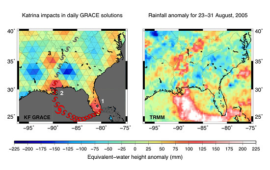
3.5. Detection of Sub-Monthly Impacts of Meteorological Events

The daily sampling of the KF GRACE solutions enables catching possible sub-monthly variations of water mass, even if a couple of days appears to be the limit of time resolution of GRACE satellite track coverage. To demonstrate this ability of detection, it is possible to consider the gravitational effects of extreme meteorological depressions lasting a couple of days that bring important rainfalls that cause heavy water storage impacts on land. In particular, the gravity anomaly signature of hurricanes reaching category 5 on the Saffir–Simpson scale that approach the southern coast of United States should be seen. The most powerful depressions in late summer 2005, named “Katrina” (23–31/08/2005), “Rita” (17–26/09/2005), and “Wilma” (15–25/10/2005), created extreme and rapid floods (see Table 1 below) during the cyclonic season in Louisiana, even though Wilma remained mostly over the Gulf of Mexico and finally passed eastward by heading to the Atlantic Ocean and had the lesser impacts on continental areas of Louisiana.
Furthermore, GRACE does not see direct tropospheric effects due to Katrina and Rita hurricanes; the direct consequences of the passage of these depressions are important rainfalls, thus causted significant storage and accumulation of water on land. If the dynamic routing of water by rivers can last a couple of days, flooded zones of progressive cumulating such as the swamps in Louisiana should gain more and more water mass during the cyclonic season
Figure 6 shows the 2005 EWH time series of the tiles on the cities of New Orleans and Memphis, which were extracted from daily KF solutions. Memphis is located in the center of the Mississippi basin. The New Orleans time series exhibits a typical (wet) cyclonic season beginning in late June after a long decay of water mass and lasting three months that contain the passages of the hurricanes. However, the New Orleans time series for 2006 does not reveal any water mass cumulating in July–September and no strong tropical depression occurred in the region of Louisiana in 2006. Sub-monthly oscillations related to weekly precipitation/evaporation and river damp discharge controls become synchronized during the wet (cyclonic) season of July–September 2005 after a continuous decrease of water mass storage, consistent with the water level records of the Mississippi River at New Orleans. During the driest season starting in June, hurricane-linked showers cause sudden peaks of water level–up to several meters for Katrina (Table 1)—of no more than one or two days (Figure 6). This suggests that the transfer of surface water is fast, and thus hardly detectable by GRACE due to the poor daily coverage of satellite tracks. Nevertheless, the Katrina and Rita periods correspond to successive accumulations of water mass amplitude of 100–150 mm of EWH each, for the New Orleans tile, by beginning the cyclonic period of 2005.
Difference maps of weekly averages of daily GRACE KF solutions and cumulated TRMM rainfalls for the periods of Katrina and Rita are presented on Figure 7. The reference map for these differences is the average taken ten days before the dominant Katrina event. Regionally-juxtaposed positive and negative anomaly patterns can be seen along and aside the hurricane-eye tracks as these two hurricanes are approaching the coast of Louisiana after having gained in humidity over the Gulf of Mexico. Positive water mass anomaly over the south of Florida is due to heavy rainfalls as Katrina tropical depression became a hurricane on 25 August; it gained in wetness over the ocean where it reached its maximum power passing in category 5. It decreased to category 3 before arriving to New Orleans on 29 August.
GRACE water storage and TRMM rainfall anomalies are generally co-localized, whereas rainfalls are simply cumulated in time at each geographical tile. The surface transfer of water, once it is on land and efficiently collected by the Mississippi River network, only lasts a couple of days. These precipitations are routed efficiently to the main stream of the Mississippi by tributaries, such as Arkansas and Red Rivers. The important rainfalls of Katrina occurring in the south of the Great Plains have generated important floods, and produced an accumulation of water up to 300 mm of EWH in the coastal region of New Orleans (see GRACE anomaly map of the right side in Figure 7).
We highlight the combined effects of rainfalls and the routing of continental waters from rivers to flooded areas. TRMM shows a large amount of rainfall (100–150 mm) over the Texas region, whereas GRACE KF solutions record a relative loss of water (-300 mm) due to a rapid transfer of surface water toward the Mississippi mouth. For Florida swamps, TRMM rainfall for the Katrina and Rita periods are low ( < 50 mm), but GRACE KF solutions show a significant accumulation of water in the swamps, i.e., topographic lows where water is trapped. An accumulation of ~100–150 mm occurs during Katrina to reach 150–200 mm during Rita. This point also reveals that the contents of TRMM and GRACE are not exactly the same: the first one mainly corresponds to the rainfalls while the second one has a content which integrates rainfalls, surface water and even groundwater. During Katrina, the continental storage is weak and the GRACE KF solutions and TRMM rainfalls are in good agreement, but, after the passage of hurricane Katrina, parts of the rain are stored in the flooded areas and flow more or less quickly towards the topographic lows, i.e., river mouths and swamps at the end. Combined with this relatively fast transfer, there are rainfalls visible on TRMM map and the accumulation of water due to Rita, and the GRACE KF solutions integrate all these effects. This explains the differences between GRACE KF and TRMM maps, in particular during hurricane Rita.

4. Conclusions

A Kalman filtering approach enables to recover the daily global variations of surface water mass over a set of triangular surfaces of constant area by progressive integration of KBRR-derived potential differences provided by the GRACE mission. This new method has been successfully applied to simulated and real GRACE RDP observations to produce successive daily global solutions of surface water mass expressed in EWH. A priori uncertainties of the KF process have to be adapted to cancel the amplification of random noise input in the simulations; while σ d acts as a regularization parameter versus noise level, σ m is a growth parameter that controls the speed of the convergence to a stable daily solution. In the case of inversion of real RDP data, series of daily global KF solutions have been produced and they reveal realistic amplitudes and locations of sub-monthly hydrological patterns even if the sparse per-day coverage of the GRACE satellite tracks limits the spatial resolution.
Future works would consist of diminishing the size of the surface tiles but unfortunately without improving the intrinsic spatial resolution of 300–400 km, while dealing with tiles (or parameters to be recovered) would require parallelization for optimizing drastically computation time. Even if sudden/extreme meteorological events of a few days remain at the limit of resolution of the GRACE data, densification of satellite tracks coverage by considering combined low altitude missions would ease the detection of large hurricanes and typhoons.
Since its successful launch in May 2018, the GRACE Follow-On mission has been ensuring the continuity of GRACE-type mass balance studies. In this context, the KF approach proposed in this article demonstrates for the first time its efficiency for monitoring extreme events, offering an interesting alternative to SH solutions by monitoring continental hydrology variations with improved regional resolutions. Combining GRACE and GRACE Follow-On data is also possible to highlight the long-term evolution of RWMC (in size, intensity, duration, and frequency) of these extreme events in the context of global warming. More investigation are required on the possible detection of gravitational signatures of such rapid mass changes by KF of GRACE-type data.

Author Contributions

Conceptualization – methodology - software, G.R and L.S.; validation - formal analysis - investigation, L.S., G.R., M.S. and J.D.; writing – original draft preparation, G.R., L.S., F.F., M.S. and E.F.; writing – review and editing, G.R., L.S., E.F. and J.D. All authors have read and agreed to the published version of the manuscript.

Funding

This research received no external funding.

Acknowledgments

We would like to thank two anonymous reviewers for having improved the quality of the manuscript by fruitful discussions about the related subject. We are also grateful to the EG2R for funding foundation RTRA STAE (grant number CDT-R053-L00-T00) to have permitted such study in global hydrology.

Conflicts of Interest

The authors declare no conflict of interest.

References

  1. Tapley, B.D.; Bettadpur, S.; Watkins, M.; Reigber, C. The gravity recovery and climate experiment: Mission overview and early results. Geophys. Res. Lett. 2004, 31. [Google Scholar] [CrossRef] [Green Version]
  2. Physical Geodesy, 2nd ed.; Hofmann-Wellenhof, B.; Moritz, H. (Eds.) Springer: Vienna, Austria, 2006; pp. 1–2. ISBN 978-3-211-33545-1. [Google Scholar]
  3. Bettadpur, S. CSR Level-2 Processing Standards Document for Level-2 Product Release 04, GRACE 327-742 (CSR-GR-03-03); The GRACE Project, Center for Space Research, The University of Texas: Austin, TX, USA, 2007. [Google Scholar]
  4. Chambers, D.P.; Bonin, J.A. Evaluation of Release-05 GRACE time-variable gravity coefficients over the ocean. Ocean Sci. 2012, 8, 859–868. [Google Scholar] [CrossRef] [Green Version]
  5. Dahle, C.; Flechtner, F.; Gruber, C.; König, D.; König, R.; Michalak, G.; Neumayer, K.-H. GFZ GRACE Level-2 Processing Standards Document for Level-2 Product Release 0005; Revised edition; GFZ Series Scientific Technical Report; GFZ Publications: Potsdam, Germany, January 2013; ISBN 1610-0956. [Google Scholar] [CrossRef]
  6. Flechtner, F. GFZ Level-2 Processing Standards Document for Product Release 0004. Rev.1.0, GRACE project documentation 327–743; GFZ: Potsdam, Germany, 2007. [Google Scholar]
  7. Vishwakarma, D.B.; Devaraju, B.; Sneeuw, N. What Is the Spatial Resolution of grace Satellite Products for Hydrology? Remote Sens. 2018, 10, 852. [Google Scholar] [CrossRef] [Green Version]
  8. Forootan, E.; Didova, O.; Schumacher, M.; Kusche, J.; Elsaka, B. Comparisons of atmospheric mass variations derived from ECMWF reanalysis and operational fields, over 2003–2011. J. Geod. 2014, 88, 503–514. [Google Scholar] [CrossRef] [Green Version]
  9. Han, S.-C.; Jekeli, C.; Shum, C.K. Time-variable aliasing effects of ocean tides, atmosphere, and continental water mass on monthly mean GRACE gravity field: Temporal aliasing on GRACE gravity field. J. Geophys. Res. 2004, 109. [Google Scholar] [CrossRef]
  10. Ray, R.D.; Luthcke, S.B. Tide model errors and GRACE gravimetry: Towards a more realistic assessment. Geophys. J. Int. 2006, 167, 1055–1059. [Google Scholar] [CrossRef] [Green Version]
  11. Thompson, P.F.; Bettadpur, S.V.; Tapley, B.D. Impact of short period, non-tidal, temporal mass variability on GRACE gravity estimates: Impact of short period, non-tidal, temporal mass variability on GRACE estimatesIMPACT OF SHORT. Geophys. Res. Lett. 2004, 31. [Google Scholar] [CrossRef]
  12. Swenson, S.; Wahr, J. Post-processing removal of correlated errors in GRACE data. Geophys. Res. Lett. 2006, 33. [Google Scholar] [CrossRef]
  13. Freeden, W.; Schreiner, M. Spherical Functions of Mathematical Geosciences: A Scalar, Vectorial, and Tensorial Setup; Advances in Geophysical and Environmental Mechanics and Mathematics; Springer: Berlin/Heidelberg, Germany, 2009; ISBN 978-3-540-85111-0. [Google Scholar]
  14. Luthcke, S.B.; Zwally, H.J.; Abdalati, W.; Rowlands, D.D.; Ray, R.D.; Nerem, R.S.; Lemoine, F.G.; McCarthy, J.J.; Chinn, D.S. Recent Greenland Ice Mass Loss by Drainage System from Satellite Gravity Observations. Science 2006, 314, 1286–1289. [Google Scholar] [CrossRef] [Green Version]
  15. Luthcke, S.B.; Sabaka, T.J.; Loomis, B.D.; Arendt, A.A.; McCarthy, J.J.; Camp, J. Antarctica, Greenland and Gulf of Alaska land-ice evolution from an iterated GRACE global mascon solution. J. Glaciol. 2013, 59, 613–631. [Google Scholar] [CrossRef]
  16. Rowlands, D.D.; Luthcke, S.B.; Klosko, S.M.; Lemoine, F.G.R.; Chinn, D.S.; McCarthy, J.J.; Cox, C.M.; Anderson, O.B. Resolving mass flux at high spatial and temporal resolution using GRACE intersatellite measurements. Geophys. Res. Lett. 2005, 32. [Google Scholar] [CrossRef]
  17. Rowlands, D.D.; Luthcke, S.B.; McCarthy, J.J.; Klosko, S.M.; Chinn, D.S.; Lemoine, F.G.; Boy, J.-P.; Sabaka, T.J. Global mass flux solutions from GRACE: A comparison of parameter estimation strategies—Mass concentrations versus Stokes coefficients. J. Geophys. Res. Solid Earth 2010, 115. [Google Scholar] [CrossRef]
  18. Watkins, M.M.; Wiese, D.N.; Yuan, D.-N.; Boening, C.; Landerer, F.W. Improved methods for observing Earth’s time variable mass distribution with GRACE using spherical cap mascons. J. Geophys. Res. Solid Earth 2015, 120, 2648–2671. [Google Scholar] [CrossRef]
  19. Wiese, D.N.; Landerer, F.W.; Watkins, M.M. Quantifying and reducing leakage errors in the JPL RL05M GRACE mascon solution. Water Resour. Res. 2016, 52, 7490–7502. [Google Scholar] [CrossRef]
  20. Wiese, D.N.; Yuan, D.-N.; Boening, C.; Landerer, F.W.; Watkins, M.M. JPL GRACE Mascon Ocean, Ice, and Hydrology Equivalent Water Height Release 06 Coastal Resolution Improvement (CRI) Filtered Version 1.0; PO.DAAC: Pasadena, CA, USA, 2018. [Google Scholar] [CrossRef]
  21. Save, H.; Bettadpur, S.; Tapley, B.D. High-resolution CSR GRACE RL05 mascons. J. Geophys. Res. Solid Earth 2016, 121, 7547–7569. [Google Scholar] [CrossRef]
  22. Jacob, T.; Wahr, J.; Pfeffer, W.T.; Swenson, S. Recent contributions of glaciers and ice caps to sea level rise. Nature 2012, 482, 514–518. [Google Scholar] [CrossRef]
  23. Schrama, E.J.O.; Wouters, B.; Rietbroek, R. A mascon approach to assess ice sheet and glacier mass balances and their uncertainties from GRACE data. J. Geophys. Res. Solid Earth 2014, 119, 6048–6066. [Google Scholar] [CrossRef]
  24. Velicogna, I.; Sutterley, T.C.; van den Broeke, M.R. Regional acceleration in ice mass loss from Greenland and Antarctica using GRACE time-variable gravity data. Geophys. Res. Lett. 2014, 41, 8130–8137. [Google Scholar] [CrossRef] [Green Version]
  25. Ramillien, G.L.; Frappart, F.; Gratton, S.; Vasseur, X. Sequential estimation of surface water mass changes from daily satellite gravimetry data. J. Geod. 2015, 89, 259–282. [Google Scholar] [CrossRef]
  26. Ramillien, G.; Biancale, R.; Gratton, S.; Vasseur, X.; Bourgogne, S. GRACE-derived surface water mass anomalies by energy integral approach: Application to continental hydrology. J. Geod. 2011, 85, 313–328. [Google Scholar] [CrossRef]
  27. Ramillien, G.L.; Seoane, L.; Frappart, F.; Biancale, R.; Gratton, S.; Vasseur, X.; Bourgogne, S. Constrained Regional Recovery of Continental Water Mass Time-variations from GRACE-based Geopotential Anomalies over South America. Surv. Geophys. 2012, 33, 887–905. [Google Scholar] [CrossRef] [Green Version]
  28. Kurtenbach, E.; Mayer-Gürr, T.; Eicker, A. Deriving daily snapshots of the Earth’s gravity field from GRACE L1B data using Kalman filtering. Geophys. Res. Lett. 2009, 36. [Google Scholar] [CrossRef]
  29. Kurtenbach, E.; Eicker, A.; Mayer-Gürr, T.; Holschneider, M.; Hayn, M.; Fuhrmann, M.; Kusche, J. Improved daily GRACE gravity field solutions using a Kalman smoother. J. Geodyn. 2012, 59–60, 39–48. [Google Scholar] [CrossRef]
  30. Sabaka, T.J.; Rowlands, D.D.; Luthcke, S.B.; Boy, J.-P. Improving global mass flux solutions from Gravity Recovery and Climate Experiment (GRACE) through forward modeling and continuous time correlation. J. Geophys. Res. Solid Earth 2010, 115. [Google Scholar] [CrossRef]
  31. Kvas, A.; Mayer-Gürr, T. GRACE gravity field recovery with background model uncertainty. J. Geod. 2019, 93, 2543–2552. [Google Scholar] [CrossRef] [Green Version]
  32. Gruber, C.; Gouweleeuw, B. Short-latency monitoring of continental, ocean-atmospheric mass variations using GRACE intersatellite accelerations. Geophys. J. Int. 2019, 217, 714–728. [Google Scholar] [CrossRef] [Green Version]
  33. Bonin, J.A.; Save, H. Evaluation of submonthly oceanographic signal in GRACE “daily” swath series using altimetry. Ocean Sci. 2019. [Google Scholar] [CrossRef] [Green Version]
  34. Rodell, M.; Houser, P.R.; Jambor, U.; Gottschalck, J.; Mitchell, K.; Meng, C.-J.; Arsenault, K.; Cosgrove, B.; Radakovich, J.; Bosilovich, M.; et al. The Global Land Data Assimilation System. Bull. Am. Meteorol. Soc. 2004, 85, 381–394. [Google Scholar] [CrossRef] [Green Version]
  35. Döll, P.; Kaspar, F.; Lehner, B. A global hydrological model for deriving water availability indicators: Model tuning and validation. J. Hydrol. 2003, 270, 105–134. [Google Scholar] [CrossRef]
  36. Güntner, A.; Stuck, J.; Werth, S.; Döll, P.; Verzano, K.; Merz, B. A global analysis of temporal and spatial variations in continental water storage. Water Resour. Res. 2007, 43. [Google Scholar] [CrossRef]
  37. Hunger, M.; Döll, P. Value of river discharge data for global-scale hydrological modeling. Hydrol. Earth Syst. Sci. 2008, 12, 841–861. [Google Scholar] [CrossRef] [Green Version]
  38. Werth, S.; Güntner, A. Calibration of a Global Hydrological Modelglobal hydrological modelwith GRACE Data. In System Earth Via Geodetic-Geophysical Space Techniques; Flechtner, F.M., Gruber, T., Güntner, A., Mandea, M., Rothacher, M., Schöne, T., Wickert, J., Eds.; Springer: Berlin/Heidelberg, Germany, 2010; pp. 417–426. ISBN 978-3-642-10228-8. [Google Scholar]
  39. Bi, H.; Ma, J.; Zheng, W.; Zeng, J. Comparison of soil moisture in GLDAS model simulations and in situ observations over the Tibetan Plateau. J. Geophys. Res. Atmos. 2016, 121, 2658–2678. [Google Scholar] [CrossRef] [Green Version]
  40. Scanlon, B.R.; Zhang, Z.; Save, H.; Sun, A.Y.; Müller Schmied, H.; van Beek, L.P.H.; Wiese, D.N.; Wada, Y.; Long, D.; Reedy, R.C.; et al. Global models underestimate large decadal declining and rising water storage trends relative to GRACE satellite data. Proc. Natl. Acad. Sci. USA 2018, 115, E1080. [Google Scholar] [CrossRef] [PubMed] [Green Version]
  41. Bruinsma, S.; Lemoine, J.-M.; Biancale, R.; Valès, N. CNES/GRGS 10-day gravity field models (release 2) and their evaluation. Adv. Space Res. 2010, 45, 587–601. [Google Scholar] [CrossRef]
  42. Lemoine, J.-M.; Bruinsma, S.; Loyer, S.; Biancale, R.; Marty, J.-C.; Perosanz, F.; Balmino, G. Temporal gravity field models inferred from GRACE data. Adv. Space Res. 2007, 39, 1620–1629. [Google Scholar] [CrossRef]
  43. Standish, E.M.; Newhall, X.X.; Williams, J.G.; Folkner, W.M. JPL Planetary and Lunar Ephermerids, DE403/LE403; JPL Inter Office Memorandum: Pasadena, CA, USA, 1995; pp. 1–22. [Google Scholar]
  44. McCarthy, D.D.; Petit, G. IERS Conventions (2003); IERS Technical Note No. 32; International Earth Rotation and Reference Systems Service (IERS): Frankfurt am Main, Germany, 2004. [Google Scholar]
  45. Wahr, J.M. Body tides on an elliptical, rotating, elastic and oceanless Earth. Geophys. J. Int. 1981, 64, 677–703. [Google Scholar] [CrossRef] [Green Version]
  46. Cartwright, D.E.; Tayler, R.J. New computations of the tide-generating potential. Geophys. J. Int. 1971, 23, 45–73. [Google Scholar] [CrossRef] [Green Version]
  47. Cartwright, D.E.; Edden, A.C. Corrected Tables of Tidal Harmonics. Geophys. J. R. Astron. Soc. 1973, 33, 253–264. [Google Scholar] [CrossRef] [Green Version]
  48. Casotto, S. Nominal Ocean Tide Models for TOPEX Precise Orbit Determination. Ph.D. Thesis, Texas University, Austin, TX, USA, 1989. [Google Scholar]
  49. Le Provost, C.; Genco, M.L.; Lyard, F.; Vincent, P.; Canceil, P. Spectroscopy of the world ocean tides from a finite element hydrodynamic model. J. Geophys. Res. Oceans 1994, 99, 24777–24797. [Google Scholar] [CrossRef]
  50. Desai, S.D. Observing the pole tide with satellite altimetry. J. Geophys. Res. Oceans 2002, 107, 7-1–7-13. [Google Scholar] [CrossRef]
  51. Carrère, L.; Lyard, F. Modeling the barotropic response of the global ocean to atmospheric wind and pressure forcing—Comparisons with observations. Geophys. Res. Lett. 2003, 30. [Google Scholar] [CrossRef] [Green Version]
  52. Jekeli, C. The determination of gravitational potential differences from satellite-to-satellite tracking. Celest. Mech. Dyn. Astron. 1999, 75, 85–101. [Google Scholar] [CrossRef]
  53. Han, S.-C.; Shum, C.K.; Jekeli, C. Precise estimation of in situ geopotential differences from GRACE low-low satellite-to-satellite tracking and accelerometer data. J. Geophys. Res. Solid Earth 2006, 111. [Google Scholar] [CrossRef] [Green Version]
  54. Evensen, G. Data Assimilation; Springer: Berlin/Heidelberg, Germany, 2009; ISBN 978-3-642-03710-8. [Google Scholar]
  55. Kalman, R.E. A New Approach to Linear Filtering and Prediction Problems. J. Basic Eng. 1960, 82, 35–45. [Google Scholar] [CrossRef] [Green Version]
  56. Kalman, R.E.; Bucy, R.S. New Results in Linear Filtering and Prediction Theory. J. Basic Eng. 1961, 83, 95–108. [Google Scholar] [CrossRef]
  57. Encarnação, J.; Klees, R.; Zapreeva, E.; Ditmar, P.; Kusche, J. Influence of Hydrology-Related Temporal Aliasing on the Quality of Monthly Models Derived from GRACE Satellite Gravimetric Data. In Proceedings of the Observing our Changing Earth; Sideris, M.G., Ed.; Springer: Berlin/Heidelberg, Germany, 2009; pp. 323–328. [Google Scholar]
  58. Arvor, D.; Funatsu, B.; Michot, V.; Dubreuil, V. Monitoring Rainfall Patterns in the Southern Amazon with PERSIANN-CDR Data: Long-Term Characteristics and Trends. Remote Sens. 2017, 9, 889. [Google Scholar] [CrossRef] [Green Version]
  59. Espinoza, J.C.; Marengo, J.A.; Ronchail, J.; Carpio, J.M.; Flores, L.N.; Guyot, J.L. The extreme 2014 flood in south-western Amazon basin: The role of tropical-subtropical South Atlantic SST gradient. Environ. Res. Lett. 2014, 9, 124007. [Google Scholar] [CrossRef]
  60. Marengo, J.A.; Liebmann, B.; Grimm, A.M.; Misra, V.; Silva Dias, P.L.; Cavalcanti, I.F.A.; Carvalho, L.M.V.; Berbery, E.H.; Ambrizzi, T.; Vera, C.S.; et al. Recent developments on the South American monsoon system. Int. J. Climatol. 2012, 32, 1–21. [Google Scholar] [CrossRef] [Green Version]
  61. Cai, W.; Cowan, T.; Thatcher, M. Rainfall reductions over Southern Hemisphere semi-arid regions: The role of subtropical dry zone expansion. Sci. Rep. 2012, 2, 702. [Google Scholar] [CrossRef] [Green Version]
Figure 1. Snapshots of daily global estimations of water mass density from WGHM-simulated potential anomalies that decrease with the number of iterations (left column), and associated absolute errors (right column).
Remotesensing 12 01299 g001
Figure 2. Daily global KF solutions computed by progressive integration of real GRACE potential differences and showing the evolution of the surface water mass density versus time.
Remotesensing 12 01299 g002
Figure 3. Amazon basin EWH time series: (a) for different sets of regularization parameters showing the impact of the surface element sizes; and (b) comparison with estimates of monthly solutions provided by the GRACE official centers.
Remotesensing 12 01299 g003
Figure 4. Time series of daily KF GRACE solutions (black) averaged over the largest drainage basins of the world. Error bars represent uncertainty on the spatial averages of daily KF solutions. Monthly estimates from the official centers CSR, GFZ, JPL, and AIUB are plotted in colors for comparison. RMS differences between one-month averaged KF values and the latter solutions are also indicated.
Remotesensing 12 01299 g004
Figure 5. Solutions for June 2006 from: (a) RL06 CSR Mascons; (b) one-month averaged EKF solutions; (c) WGHM model output; and (d) GLDAS model output.
Remotesensing 12 01299 g005
Figure 6. (Top) Time series of EWH for surface tiles centered on the cities of New Orleans and Memphis extracted from the daily KF solutions. Error bars represent final uncertainties (about 0.1 mm for each triangular tile). The spin-up delay from cold start of the KF process is not represented here. The weekly periods of the main 2005 hurricanes during the cyclonic period (three-month bulge) are shaded. (Bottom) Historic daily records of Mississippi River level at New Orleans (Carrollton stage) collected by the Water Control Center, New Orleans District—US Army Corps of Engineers (http://rivergages.mvr.usace.army.mil/WaterControl/).
Remotesensing 12 01299 g006
Figure 7. Differences of weekly-averaged KF solutions before and during the Katrina and Rita passages (top); and comparison with the anomalies of TRMM precipitation for the same periods (bottom). Daily rainfall maps are provided by NASA (https://pmm.nasa.gov/data-access/downloads/trmm). Katrina and Rita paths are extracted from the NOAA website (http://www.climate.gov). Grey and red symbols are for tropical depression and category 5 hurricane, respectively. The KF solution difference maps reveal the positive and negative variations of water mass along the paths of the depressions that cause strong showers. The highest water storage variation is located in the coastal region of Louisiana.
Remotesensing 12 01299 g007
Table 1. Main characteristics of Katrina, Rita and Wilma Hurricanes that hit the coasts of Florida and Mississippi.
NameDateLowest Pressure 1 (hPa)Max. Surge Flooding (m)Max. Wind Speed (km/h)Max. Rainfall (mm)
Katrina23–31/08/20059028.2 Mississippi Coast~200 Southeast Louisiana 3 198 in 48 h Philpot 3
Rita17–26/09/20058951.5 Key West185 South Louisiana130
Wilma15–25/10/2005882 Record low in the Atlantic1.98 Key West 219076
1 Atlantic hurricane best track (HURDAT version 2) U. S. A. National Hurricane Center. December 12, 2019. 2 Kasper, 2007, Hurricane Wilma in the Florida Keys, NOAA/NWS Weather Forecast Office (WFO) Key West. 3 Jeffrey Medlin, Ray Ball, and Gary Beeler. Updated by Morgan Barry, Jason Beaman, and Don Shepherd, November 2016, Hurricane Katrina—August 2005, National Weather Service, https://www.weather.gov/mob/katrina.

