Spatially Enhanced Spectral Unmixing Through Data Fusion of Spectral and Visible Images from Different Sensors

Abstract

We propose an unmixing framework for enhancing endmember fraction maps using a combination of spectral and visible images. The new method, data fusion through spatial information-aided learning (DFuSIAL), is based on a learning process for the fusion of a multispectral image of low spatial resolution and a visible RGB image of high spatial resolution. Unlike commonly used methods, DFuSIAL allows for fusing data from different sensors. To achieve this objective, we apply a learning process using automatically extracted invariant points, which are assumed to have the same land cover type in both images. First, we estimate the fraction maps of a set of endmembers for the spectral image. Then, we train a spatial-features aided neural network (SFFAN) to learn the relationship between the fractions, the visible bands, and rotation-invariant spatial features for learning (RISFLs) that we extract from the RGB image. Our experiments show that the proposed DFuSIAL method obtains fraction maps with significantly enhanced spatial resolution and an average mean absolute error between 2% and 4% compared to the reference ground truth. Furthermore, it is shown that the proposed method is preferable to other examined state-of-the-art methods, especially when data is obtained from different instruments and in cases with missing-data pixels.

1. Introduction

Imaging spectrometers collect a large number of samples of the reflected light at different wavelengths along the electromagnetic spectrum [1]. Accordingly, each pixel of the spectral image holds a spectral signature that describes the chemical and physical characteristics of the surface [2]. This amount of valuable information can be used in critical image-based geoscience applications [3]. Unfortunately, the spatial resolution (SR) of remotely sensed spectral images is low, thus limiting the accuracy of the outcomes of spectral data applications [4,5,6,7], e.g., classification, unmixing, target and object detection, mineralogy, and change detection.

On the other hand, the full information provided by spectral images enables the extraction of quantitative subpixel information. One crucial and useful technique for this purpose is spectral unmixing [8,9]. Using this technique, the abundance fraction of each distinct material, i.e., a so-called endmember (EM), is estimated for each pixel in a given spectral image. The achieved subpixel information is essential for the quantitative analysis of pixel content. Traditional unmixing methods rely only on the spectral data of the image, whereas spatially adaptive methods also incorporate the spatial information of the image to enhance the accuracy of the estimated fraction. In both cases, however, there is no information regarding the spatial distribution of the EMs within the pixel area and so the SR of the extracted fraction maps is also limited and is as low as the SR of the spectral image.

Moreover, all existing frameworks for unmixing do not allow the incorporation of information from external sources, e.g., visible images. Fusion of two data sources to enhance the SR of spectral images is, however, a conventional practice in the field of remote sensing. Indeed, many techniques are available for enhancing the SR of the entire spectral image; one useful technique for this purpose is pan sharpening (PS) [10].

The PS process relies on data fusion of a low SR (LSR) spectral image and a corresponding high SR (HSR) panchromatic image. A variety of PS methods have been developed [10,11] and a general classification of which yields three main types [12]: component substitution-based methods, e.g., [13], multiresolution analysis-based methods, e.g., [14,15], and optimization-based approaches, e.g., [16]. Despite the availability of multiple PS methods, some significant limitations still exist, such as spectral distortion, spatial distortion, and the need for prior information. To overcome these drawbacks, advanced neural network (NN)-based algorithms have been introduced, mainly over the past two decades. NNs offer ways to fuse different data sources with a minimal need for prior assumptions [17]. Some of these algorithms rely on fully connected feedforward NNs, e.g., [18,19], but the majority were developed based on convolutional NNs (CNNs) [12,20,21,22,23,24,25].

The use of the CNN-based approach has proven to improve the PS process significantly; one pioneer method in this regard is the Pansharpening by Convolutional Neural Networks (PNN) presented in [25]. PNN utilizes a relatively shallow network with the incorporation of extra information through maps of nonlinear radiometric indices. Since [25] was proposed, a variety of works addressed the application of PS based on CNNs. For instance, in [26], the PNN is used as a baseline. Then, a further improvement of the results is achieved by adding a fine-tuning layer within the network. Furthermore, other methods have been developed by addressing specific limitations of earlier practices. For example, among the most recent works, the proposed CNN architecture in [27], relies on the hierarchical pyramid structure to derive more robust features for better retrieval of HSR multispectral images. Whereas the proposed CNN in [28] is intended for detail-preserving through a cross-scale learning strategy, the applied strategy in [29] is based on a progressive cascade deep residual network to reduce the loss of high-frequency details. Finally, while most of the methods utilize shallow networks to prevent the effect of vanishing gradient, [30,31], the presented approach in [32] allows for using very deep CNNs based on dense blocks and residual learning. The potential of deeper networks to characterize and map challenging relationships between the fused data is assumed to be higher than that of shallow NNs.

Although the use of NNs leads to enhanced PS results compared with conventional methods, all existing PS algorithms require both spatial and temporal overlapping between the spectral and panchromatic images, a condition that is, in most cases, extremely challenging to fulfill. Thus, PS methods are limited to data sets acquired by the same instrument. The work presented in [33] reports the sensitivity of PS methods to temporal and instrumental changes between spectral and panchromatic data sets. Moreover, since PS retrieves a full HSR spectral image, the applied process is usually complicated and time-consuming. In addition, CNNs typically are designed and trained for specific types of images and, thus, do not fit for application to new data sources.

In this work, we present a new methodology for enhancing the SR of abundance fraction maps by fusion of spectral and visible images from different sensors. Traditional unmixing methods rely only on the spectral image and so the fraction maps obtained provide valuable quantitative subpixel information but with the same (usually low) SR of the image itself. Addressing this limitation, we propose a new framework that combines the spectral unmixing approach with machine learning for modeling the relationship between the EM fractions and the RGB values. In this regard, the proposed workflow allows for using different learning mechanisms for multivariate regression. Here we use an NN for this purpose due to its little need for prior assumptions. Furthermore, NNs were found in many cases to outperform standard machine learning procedures in solving remote sensing tasks, as shown, for example, in [34]. Unlike traditional methods, we fuse data sources without full spatial, spectral, and temporal overlapping between the two data types. We use spectral and spatial information that we extract from the involved data sources without any further information or assumptions. For this purpose, we design a new spatial features-aided neural network (SFANN). In particular, NNs provide an efficient tool for fusing different types of remote sensing data images. Due to the different conditions, different sensors, and a probable difference in acquisition dates, the images from the two data sources must be coregistered geometrically and calibrated radiometrically. In practice, even after coregistration, the pixels in the data sources do not perfectly match due to errors in the process itself and real changes in the land cover of the surface. Feeding the NN with data from mismatching pixels will lead to an error in the results. To prevent possible data mismatches, we propose a new strategy that does not require coregistration between the images. Instead, we use what we call invariant points (IPs), i.e., points that appear in the two images and represent features that are robust to the different acquisition conditions. We, therefore, examined different methods of IP extraction and found that the scale-invariant feature transform (SIFT) method [35] provides the best results for the data we use in our experiments. First, we use these IPs to radiometrically calibrate the RGB values in preprocessing. Then, we feed the SFANN with the calibrated RGB values and spatial features (SFs) of the IPs in the visible image, as input data, and with their corresponding fraction values, as target data. Finally, we derive the fraction values of the EMs from the LSR fraction maps obtained by the unmixing of the spectral image The proposed method is, to the best of our knowledge, the first to be developed using SFANN for the enhancement of the SR of a specific spectral product, the fraction maps in our case. This paper contributes in three main aspects:

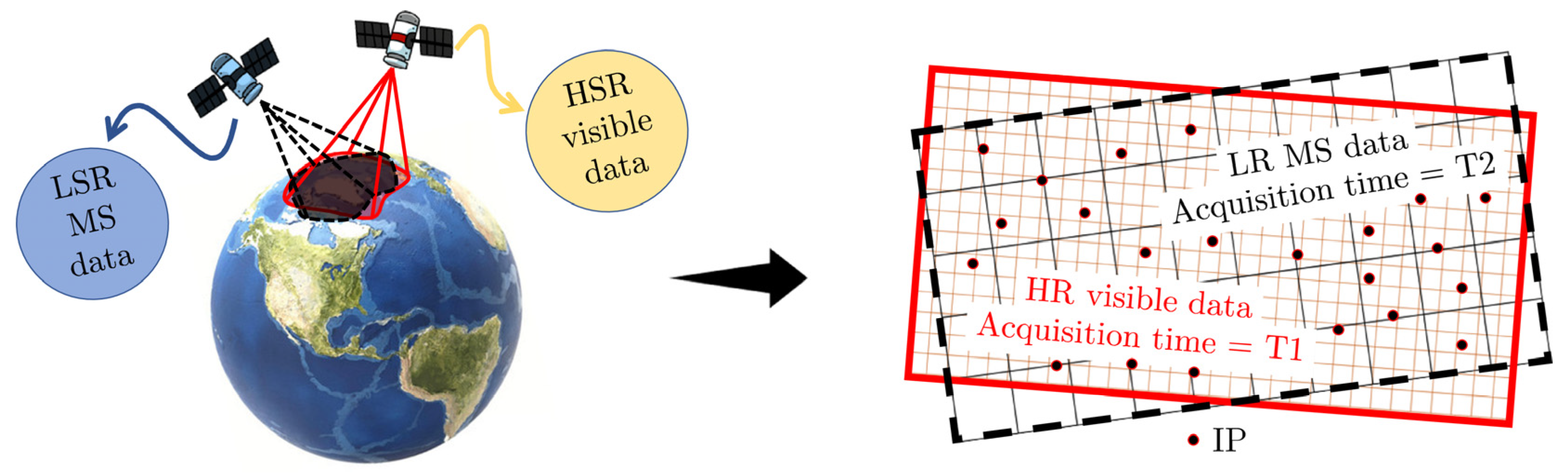
• We propose a computationally light strategy for the fusion of data from different sensors without the need for full spatial, spectral, and temporal overlapping.
• We introduce a new rotation-invariant spatial feature for learning (RISFL) that allows for the incorporation of spatial information within the machine learning process without the need for CNNs.
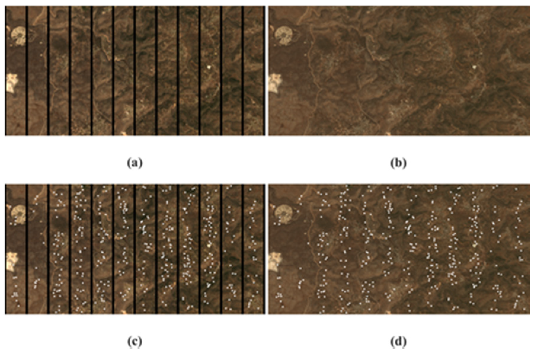
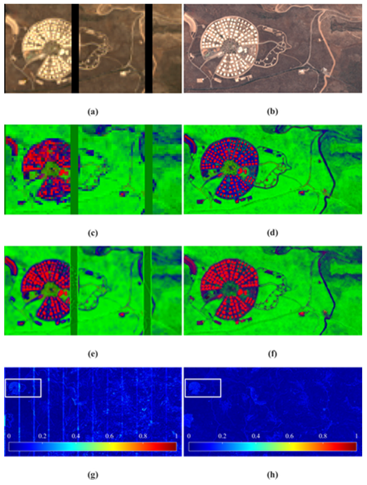
• Using IPs, as proposed in the paper, we suggest a new strategy for data fusion that allows for the use of sources with missing-data pixels, e.g., images provided by Landsat 7 with data gaps due to scan line corrector failure [36].

The proposed framework provides a beneficial tool that we predict will be very relevant for new remote sensing tasks that rely on data from different instruments. This relevance keeps increasing due to the continual development of different sensing platforms, including satellites and airborne and unmanned aerial vehicles. To demonstrate and evaluate the performance of the new technique, we use spectral images provided by Landsat 8, Sentinel 2 A, Venus, GeoEye-1, Ikonos, and WorldView-2 satellites as well as a Google Earth RGB image of high SR.

2. Materials and Methods

2.1. Spectral Unmixing

Spectral unmixing allows for extracting subpixel information by estimating the abundance fractions for a set of EMs. Let $\lambda$ and $d$ denote the number of bands in a spectral image and the number of EMs to be used for the unmixing, respectively, and following the linear mixture model, the spectral signature of each pixel, $m={[m_1,\dots ,m_{\lambda }]}^T$, is given by:

$$m=Ef+n.$$

(1)

Given the pixel’s spectral signature $m$, the matrix of EMs $E\in {ℝ}^{\lambda \times d}$, and assuming that $n\in {ℝ}^{\lambda \times 1}$ represents a zero mean Gaussian noise, an estimation of the fraction vector $f\in {ℝ}^{d\times 1}$ is achieved by minimizing the following fidelity term:

$$\widehat{\mathbf{f}}=\underset{\mathrm{f}}{\arg \min }\left(\frac{1}{2}{\Vert Ef-m\Vert }_2^2\right).$$

(2)

Requesting a physically feasible solution, the estimation needs to be subject to the abundance non-negativity constraint and the abundance sum-to-one constraint [37], i.e., ${\widehat{\mathbf{f}}}_i\ge 0$ for $i=1,\dots ,d$ and ${\widehat{\mathbf{f}}}^{{\rm T}}1\le 1$, respectively, where $1\in {ℝ}^{d\times 1}$ is a vector of ones. The optimization problem in Equation (2) represents a basic form of supervised unmixing without any regularization. In practice, different objective functions can also be used [38,39], and sparse [40] and spatial [41] regularizations are promoted within a modified objective function to enhance result accuracy. In addition to the influence of the selected optimization process, the accuracy of the used EMs also affects the accuracy of the obtained solution. Although a set of EMs can be selected from a spectral library, EMs that are extracted from the image itself [42] are usually preferred since they share acquisition conditions with the image pixels. The fraction maps obtained from the unmixing process provide valuable quantitative information. However, due to the use of the spectral image only, the SR of these maps is usually low. Our purpose is to enhance the SR by fusing the spectral image with a visible image of HSR.

2.2. Invariant Points (IPs) for Supervised Learning and Fusion of Data from Different Sensors

Traditional methods for image data fusion in remote sensing usually require full (spatial and temporal) overlapping of the data sources. This constraint of using fully overlapping images prevents the use of data from different instruments causing us to miss the opportunity to use multiple available data combinations for data fusion tasks. In some cases, these data types are even available without charge, e.g., images from Landsat, Sentinel, and Google Earth. Figure 1 illustrates the limitation of using images from different instruments for traditional data fusion.

Addressing this limitation, we suggest using IPs for a fusion process that is robust to probable mismatches between the data sources. In practice, an IP represents a point that can be detected in both images and has the same land cover type in both images. In other words, IPs are invariant to both geometrical and temporal changes in the data due to the acquisition conditions. We therefore use IPs for robust learning of the pattern that connects the HSR RGB values to the fraction values derived from the LSR multispectral (MS) image. In addition, the proposed IP-based learning is robust to probable missing-data pixels, i.e., pixels with no information in the image, for example, due to the presence of clouds or sensor malfunction [43,44].

2.3. Automatic Extraction of IPs

The use of IPs is essential for connecting the fused data sources, first for calibrating the RGB image to the spectral image and then to feed the SFANN with reliable input and target data. To obtain robust IPs, we apply a two-step strategy that combines; (1) an automatic method for extracting matching points and, (2) the random sample consensus (RANSAC) algorithm [45] to detect incorrect pairs of key points due to a probable mismatch in the previous step (see [46] for more details about all the steps in the IP extraction part). Several automatic methods are suitable for IP extraction. Among the three examined methods in our experiments, SIFT, speeded-up robust features (SURF) [47], and binary robust invariant scalable keypoints (BRISK) [48], the results obtained with SIFT were advantageous in regard to accuracy and number of extracted IPs. Quantitively, the number of IPs detected by SURF or BRISK is between 40% and 80% of the extracted IPs by SIFT. Nevertheless, this conclusion stands only for the datasets we used in our experiments, and one should always test different methods for different datasets.

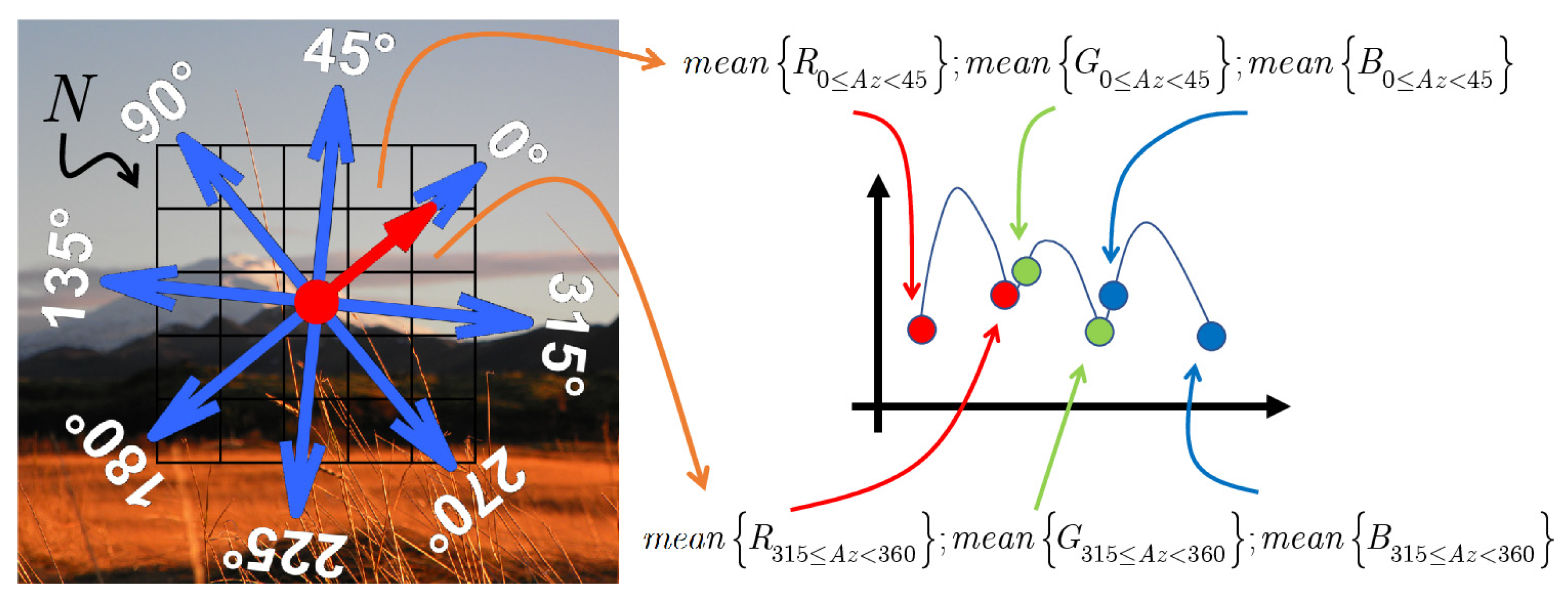
2.4. Rotation Invariant Spatial Features for Learning for the Incorporation of Spatial Information

In natural scenes, important spatial information is inherent in the 2 D distribution of the image pixels. Combining this information within the unmixing process significantly improves results [49]. An efficient way of combining spatial information within a machine-learning process is by using CNNs. These, however, are usually complex, computationally heavy, and require a large number of training data samples, which are not always available. For example, in the proposed framework, the number of extracted IPs is probably insufficient for training a CNN. We therefore prefer to use a simpler learning mechanism, e.g., a feedforward NN. Then, to incorporate the spatial information of the images into the learning process, we map the 2D spatial information into a 1D vector. Unlike descriptors that are designed to match or categorize images, the desired spatial feature (SF) is intended for learning. In addition, we expect it to provide similar results for similar objects that may appear in the image in different orientations. The introduced variance in the data due to probable rotations of objects from the same class and the advantage of using rotation-invariant features to minimize the complexity of the learning process in this regard is addressed and presented well in [46]. Thus, the proposed SF must have the two following properties:

• Be robust to rotation.
• Maps the spatial distribution of the original colors surrounding the pixels.

For this purpose, we define a new rotation-invariant spatial feature for learning (RISFL) that we extract by calculating the spatial distribution of colors in the local neighborhood surrounding each pixel in an RGB image. In other words, the RISFL maps the directional distribution of the colors surrounding the pixel. To set a reference direction that is robust to probable rotations of the objects in the image, we use the gradient of color intensity around the pixel. Specifically, given three sets of values, $V_r$, $V_g$ and $V_b$, that respectively represent the R, G, and B values of the pixels within a specified neighborhood, $N$, surrounding pixel $\left(x_c,y_c\right)$ (see Figure 2), we calculate the RISFL for the center pixel in $N$ as follows:

• Compute the direction (azimuth) of the local gradient, i.e., $A{z}_G$, at the pixel $\left(x_c,y_c\right)$.
• Calculate the azimuth to each pixel in $N$ in a local coordinate system centered at pixel $\left(x_c,y_c\right)$ and rotated by $A{z}_G$, such that the new azimuth of the gradient direction is zero.
• Divide $N$ into $n$ directional regions (see Figure 3), $\left\{S_1,S_2,\dots ,S_n\right\}$, such that

  $$S_i=\left\{P\in N|\left(i+1\right)·\frac{2\pi }{n}\le Az\left(x_p,y_p\right)<i·\frac{2\pi }{n}\right\}$$

  (3)

  where $P\in N$ is a set of pixels within $N$, and $Az\left(x_p,y_p\right)$ is the local azimuth of the pixel at location $\left(x_p,y_p\right)\in N$. For example, let $n=8$. The first directional region, $S_1$, will include all pixels in $N$ with azimuth values equal to or greater than $0°$ and smaller than $45°$, and the last directional region, $S_8$, will include all pixels with azimuths equal to or greater than $315°$ and smaller than $360°$(see Figure 2)
• For each region, calculate the mean value of the R, G, and B for all pixels that fall within the region.

Figure 2 illustrates the main concepts of computing the proposed RISFL.

The number of elements in the obtained RISFL is constant for a given number of directional regions ($n$), regardless of the neighborhood’s size ($N$). Thus, the method allows for experimenting with different sizes of $N$, for the same value of $n$, without modifying any of the other elements of the learning framework.

Although the use of more directional regions is assumed to enable the extraction of more detailed RISFLs, the use of large values of $n$ for small values of $N$ is not practical. We should, therefore, consider the balance between these two parameters when designing the learning framework. Figure 3 and Figure 4 further illustrate the steps for computing the proposed RISFL for a pixel in an area with an edge and in a homogenous area, respectively, at different degrees of rotation.

In both cases, the robustness of the RISFL to rotation is evident. Moreover, Figure 4 shows that the error in calculating the azimuth gradient in homogenous areas may be relatively large. For example, the azimuth of the gradient at the central pixel under a $0°$ rotation is $7.8°$. Thus, the azimuth under a $45°$ rotation is supposed to be $52.8°$, whereas the calculated azimuth is $44.8°$, i.e., an error of $8°$. Since the area is homogenous, however, the influence of this error on the obtained RISFL is minor, as observed from the presented features under the different rotations (tiles g–i). Although at this time we use only the mean value for each region, the RISFL allows the use of any other statistic or metric regarding the colors, e.g., variance, range, and covariance between the different colors.

2.5. Empirical Line Calibration

We use the empirical line calibration [50,51] to convert the unit-less DN values from the RGB image into reflectance units as follows:

$${\rho }_{\lambda }={\alpha }_{\lambda }·D{N}_{\lambda }+{\beta }_{\lambda }$$

(4)

where ${\rho }_{\lambda }$ and $D{N}_{\lambda }$ are the reflectance and DN values in the spectral band $\lambda$, respectively, and ${\alpha }_{\lambda }$ and ${\beta }_{\lambda }$ are the calibration coefficients for band $\lambda$. We use a robust fitting procedure to estimate the calibration coefficients using the extracted IPs between the images as presented in [51]. Then, we apply the estimated coefficients to all pixels in the RGB image to obtain their reflectance values. The calibration step contributes to the overall fusion process mainly by reducing the complexity of the pattern that the system needs to learn. Additionally, the robust fitting in this step helps to eliminate further outlier IPs, which may exist due to mismatches between key points in the IP extraction stage.

2.6. Data Fusion for Resolution Enhancement of Fraction Maps

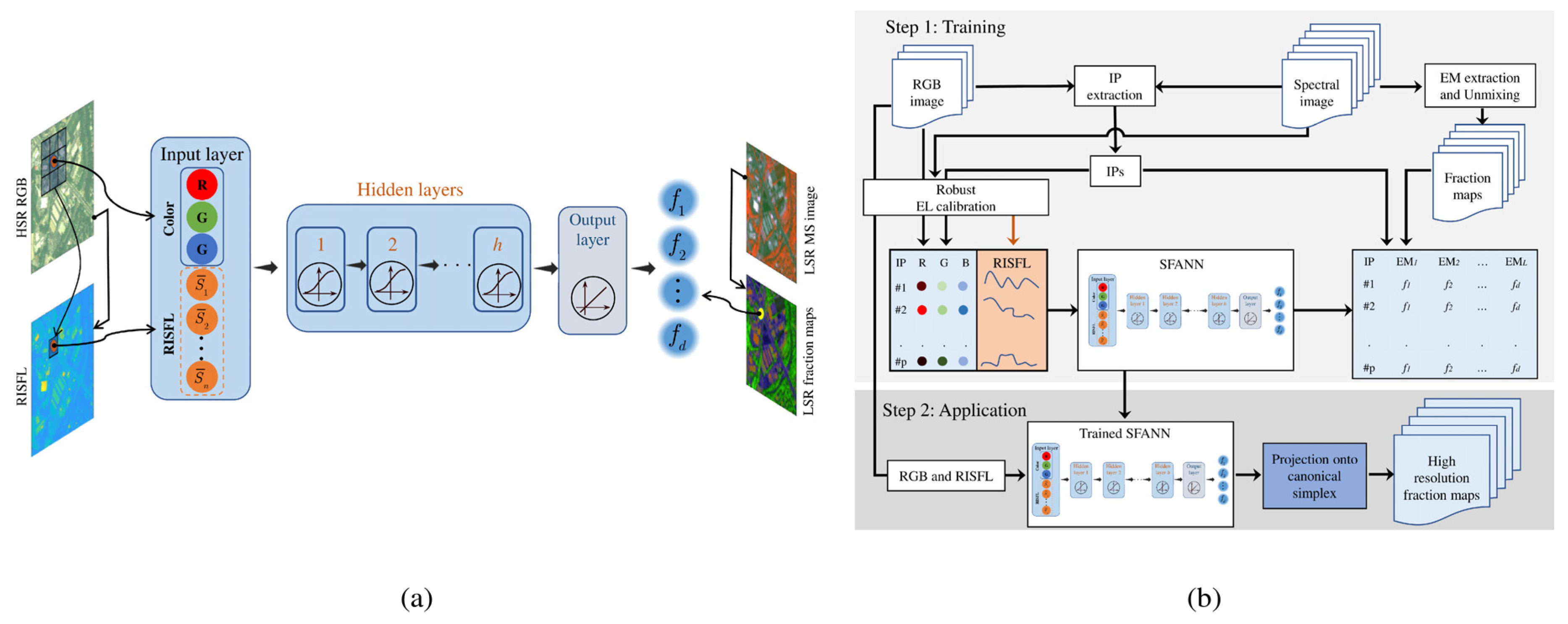
2.6.1. SFANN for Fraction Estimation

NNs are very useful for mapping relationships between input and target observations due to their high capability to learn intricate and hidden patterns within data. Relying on the insights from previous research in this regard, we decide to use a SFANN, based on a fully connected feed-forward NN (FCFFNN) to estimate the fraction values for each pixel in the HSR RGB image. The designed SFANN is intended to map the relationship between input data from the HSR image and the corresponding data from the spectral image. To fulfill the need for feeding the SFANN with a sufficient amount of training samples, we use IPs to derive this desired data from the images to be used for the fusion, with no need for any further data from additional sources.

The advantages of using FCFFNNs for the addressed fusion task are mainly the simple implementation and intuitive understanding of the network components. In practice, the three main components to be considered when designing an FCFFNN are the number of hidden layers (the depth of the network), the number of neurons in each of these layers, and the transfer function.

In comparison, CNNs usually require considering a much higher number of components and parameters when designing a new network. On the other hand, the use of spatial information in CNNs is inherent through convolution operations. In this regard, our challenge is to take advantage of the relatively simple design of FCFFNNs while also integrating the spatial information within the learning process. In practice, we incorporate additional information into the FCFFNN by concatenating the corresponding data to the 1D array of each (current) data sample (see Figure 5). The main disadvantage of this approach is, however, that each new data element increases the number of connections (weights) that we must adjust during the training process. We therefore propose a RISFL with only a moderate number of elements that sufficiently describe the spatial information in the pixel’s neighborhood. Considering the architecture of an FCFFNN, the main two elements that need to be examined are the number of hidden layers and the number of neurons in each layer. On the one hand, a high number of hidden layers increases the ability of the network to learn a more complex function. On the other hand, it may lead to a vanishing gradient problem [30,31], whereby the neurons of the earlier layers learn very slowly, making the training process impractical. Similarly, more neurons in the hidden layers allow for the fitting of more complex functions but require a massive amount of training data, potentially leading to undesired overfitting. Thus, these two aspects, among others, should be considered when designing a new network. See [52] for a detailed discussion on the FCFFNN.

We design an SFANN that fuses spectral and visible data. The SFANN notably allows for learning the connecting pattern between the pixel’s R, G, and B values and its RISFL and the corresponding fraction values from the LSR spectral image. Figure 5a presents a graphical description of the proposed SFANN.

Each input sample includes the RGB values $\in {ℝ}^{3\times 1}$ and $\mathrm{RISFL}\in {ℝ}^{3n\times 1}$, where $n$ is the number of directional regions used for the RISFL. The number of neurons in the input layer is, therefore, $c_1=3n+3$. Accordingly, let $h$ and $d$ denote the number of hidden layers and the number of EMs in the image, respectively. The number of neurons in the output layer is then $c_{h+2}=d$. Whereas a different number of neurons in the hidden layers, $c$, can be tested.

Here, we use an FCFFNN with a constant number of neurons in the hidden layers, i.e., $c_k=c$ for $k=2,\dots ,h+1$, and the log-sigmoid function (logsig) as a transfer function:

$$\mathrm{logsig}\left(x\right)=1/\left(1+e^{-x}\right)$$

(5)

While the pure linear (purelin) function is used for the output layer:

$$\mathrm{purlin}(x)=x.$$

(6)

To train the SFANN, we use the Levenberg–Marquardt backpropagation algorithm [53] to minimize the mean square error. For this purpose, we feed the network with a set of IPs that is divided into three subsets: for training, validation, and testing, with respective ratios of 70%, 15%, and 15%. Although we use RGB values and RISFLs here, we could easily incorporate different spatial features within the proposed scheme, e.g., local binary pattern features [54] and the histograms of oriented gradients [55], as well as additional input data from other sources.

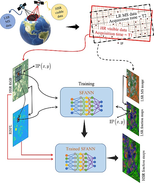
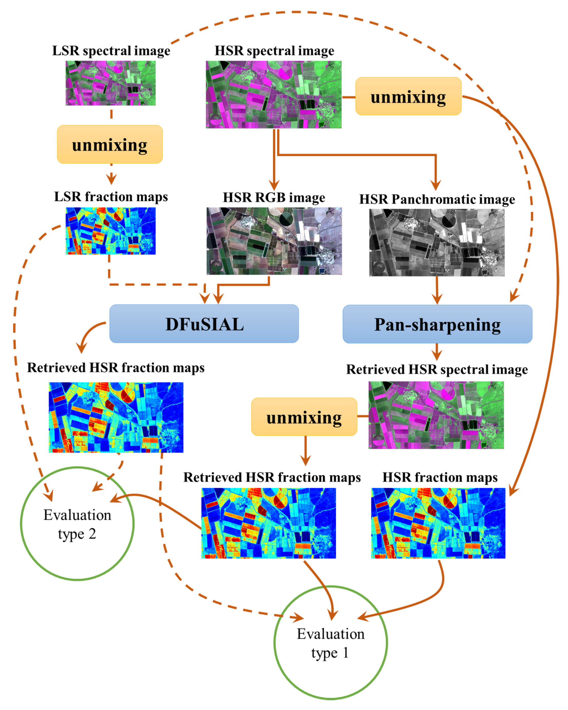
2.6.2. Methodological Framework

Given a spectral image with low SR and a visible image with HSR, we use these two types of data to extract fraction maps with enhanced SR. In practice, we use the described SFANN to fuse the two data sources by modeling the relationship between the RISFLs and the fractions of each EM and the RGB values, as follows:

• Extract IPs between the spectral and visible RGB images.
• Calibrate the RGB values using robust empirical line (EL) calibration.
• Extract RISFLs.
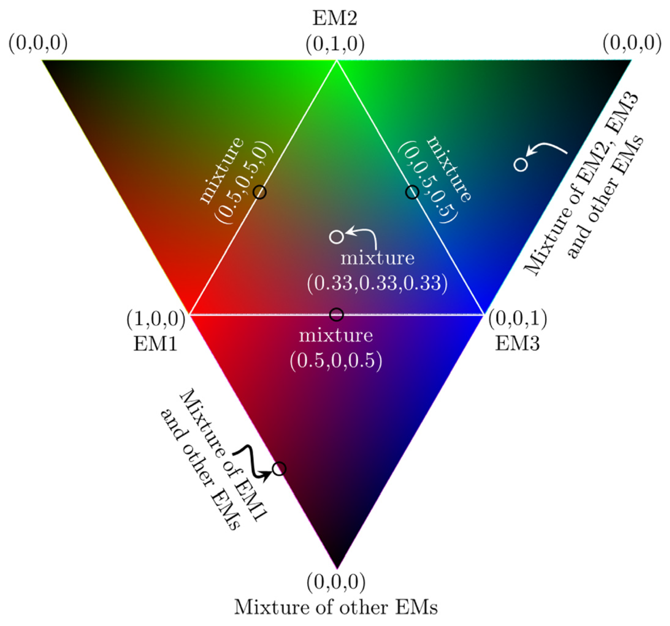
• Automatically extract EMs from the spectral image.
• Estimate the fraction map for each EM using the unmixing process.
• Using the IPs, train the SFANN to model the relationship between the calibrated RGB values, the RISFLs, and the fractions of each EM.
• Apply the trained SFANN to all pixels in the visible image and their RISFLs to create fraction maps with HSR.
• Apply the abundance non-negativity and sum-to-one constraints to provide fully constrained fractions. For this part, we project the output fractions onto the canonical simplex [56], as presented in [38] and [57].

Here we use the vertex component analysis (VCA) [58] method to extract EMs and the sparse unmixing by variable splitting and augmented Lagrangian (SUnSAL) [59] method to estimate the fraction, though any other combination of different methods may be efficiently implemented within the proposed framework as well. In addition to its significantly fast performance, VCA can estimate EMs also in the absence of pure pixels in the scene and so is preferable for cases of LSR in which the presence of pure pixels is not highly probable. SUnSAL is computationally light and has the advantage of yielding a sparse solution. Figure 5b presents the framework of the proposed methodology.

2.7. Data and Experimental Evaluation

To evaluate the proposed methodology, we use seven data sets:

• A spectral image with seven bands and an SR of 30 m (Figure 6a), provided by the Landsat 8’s Operational Land Imager (OLI), and a corresponding spectral image of the same area with SR of 10 m provided by the Sentinel 2 A satellite (Figure 6b).
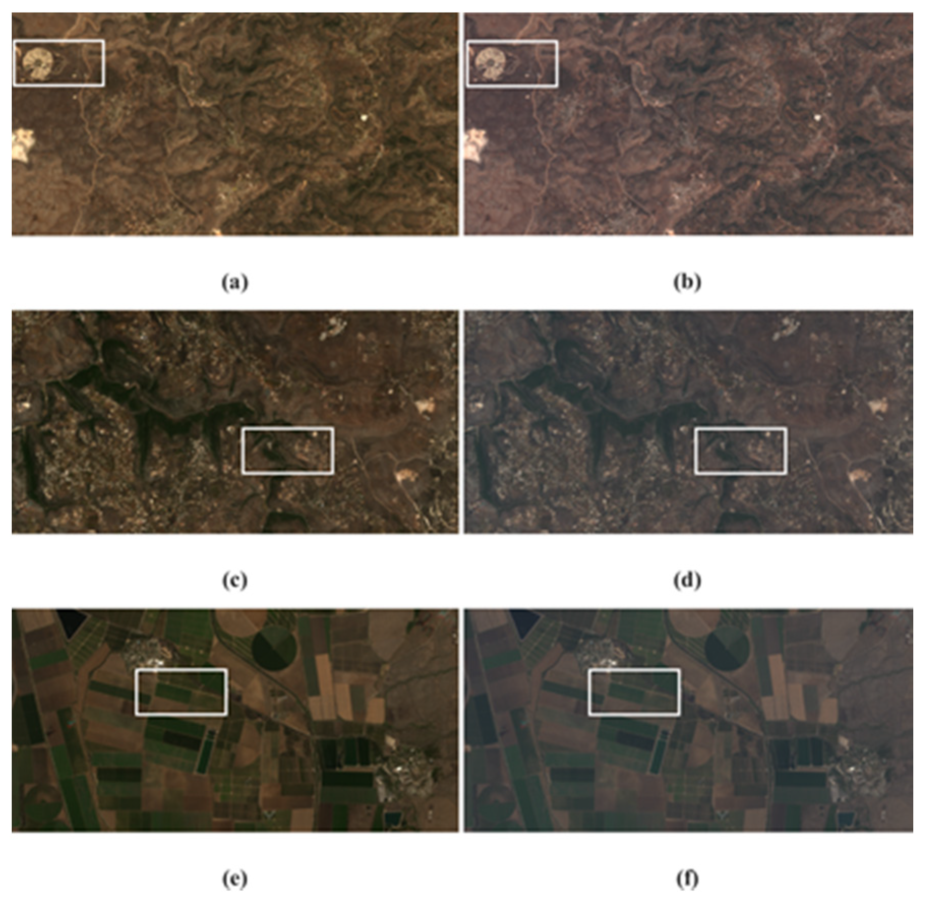
• Venus dataset-a, a spectral image with 12 bands and an SR of 10 m along with its corresponding uncalibrated spectral image with an SR of 5 m, both provided by the Venus satellite (Figure 6c,d).
• Venus dataset-b, similar to data set #2 but for a different area that contains multiple homogeneous regions (Figure 6e,f).
• A spectral image provided by the GeoEye-1 satellite with four bands and SR of 1.84 meters and a corresponding panchromatic image with SR of 0.46 m.
• A spectral image provided by the Ikonos satellite with four bands and SR of 3.28 meters and a corresponding panchromatic image with SR of 0.82 m.
• A spectral image provided by the WorldView-2 satellite with eight bands and SR of 1.84 meters and a corresponding panchromatic image with SR of 0.46 m.
• An RGB image, with an SR of 1 m, available for free, on Google Earth and a corresponding spectral image of the same area with SR of 10 m provided by the Sentinel 2 A satellite.

We divide the seven datasets into three groups according to the availability and type of reference ground truth that we use for the evaluation as following:

• Group-1 includes datasets 1, 2, and 3. In each of these three cases, a real full-reference HSR spectral image is available and used for the evaluation of the obtained HSR fraction maps.

  -

  The Sentinel image has 13 bands: 1–8, 8 A, and 9–12. The central wavelength of bands 1–4, 8 A, 11, and 12 is similar to that of the Landsat bands and so we use these bands in our experiments. The visible bands, 2, 3, and 4, have an SR of 10 m and were used to create a corresponding RGB image. The resolution of bands 1, 8 A, 11, and 12 was artificially resampled from 20 m to 10 m. The Landsat image was acquired on 28 May 2017, whereas the Sentinel image was acquired three days later, on 31 May 2017.

  -

  The second and third datasets combine fully overlapping images that were simultaneously acquired on 17 June 2018 by the Venus satellite. The satellite provides the LSR (10 m) image with reflectance units, while the HSR (5 m) image is available only with uncalibrated DN units.

• Group-2 includes datasets 4, 5, and 6. Since a real full-reference is not available for these images, we adopted the strategy presented in [25] and [26] following Wald’s protocol [60] for generating simulated full-reference. We reduced the SR of the original data by resampling the spectral and panchromatic images in these datasets by a factor of 0.25 to create new spectral images for GeoEye-1, Ikonos, and WorldView-2 with SR of 7.36 m, 13.12, and 7.36 m, respectively. The original MS image is then used as a reference ground truth.
• Group-3 includes data set 7. The RGB image, taken from Google Earth, was acquired on 08/08/2014 and is the most recent available HSR image of the selected area. A corresponding spectral image was derived from the Sentinel-2 A image with SR of 10 m from dataset 1. No reference ground truth is available in this group.

Figure 6. presents an RGB composite of the images from datasets 1, 2, and 3, and Figure 7 shows an RGB composite of the images from datasets 4, 5, and 6. Whereas the images from dataset 7 are presented within the results of Experiment 3.

Comparing to the state-of-the-art

An alternative to the DFuSIAL for enhancing the SR of the unmixing fraction maps, through data fusion of visible HSR and spectral LSR images, is based on the PS technique. Using PS, we first retrieve an HSR spectral image and then apply the unmixing process to obtain HSR fraction maps. To analyze the performance of the DFuSIAL versus the state-of-the-art, we use two of the recent PS methods:

(1)

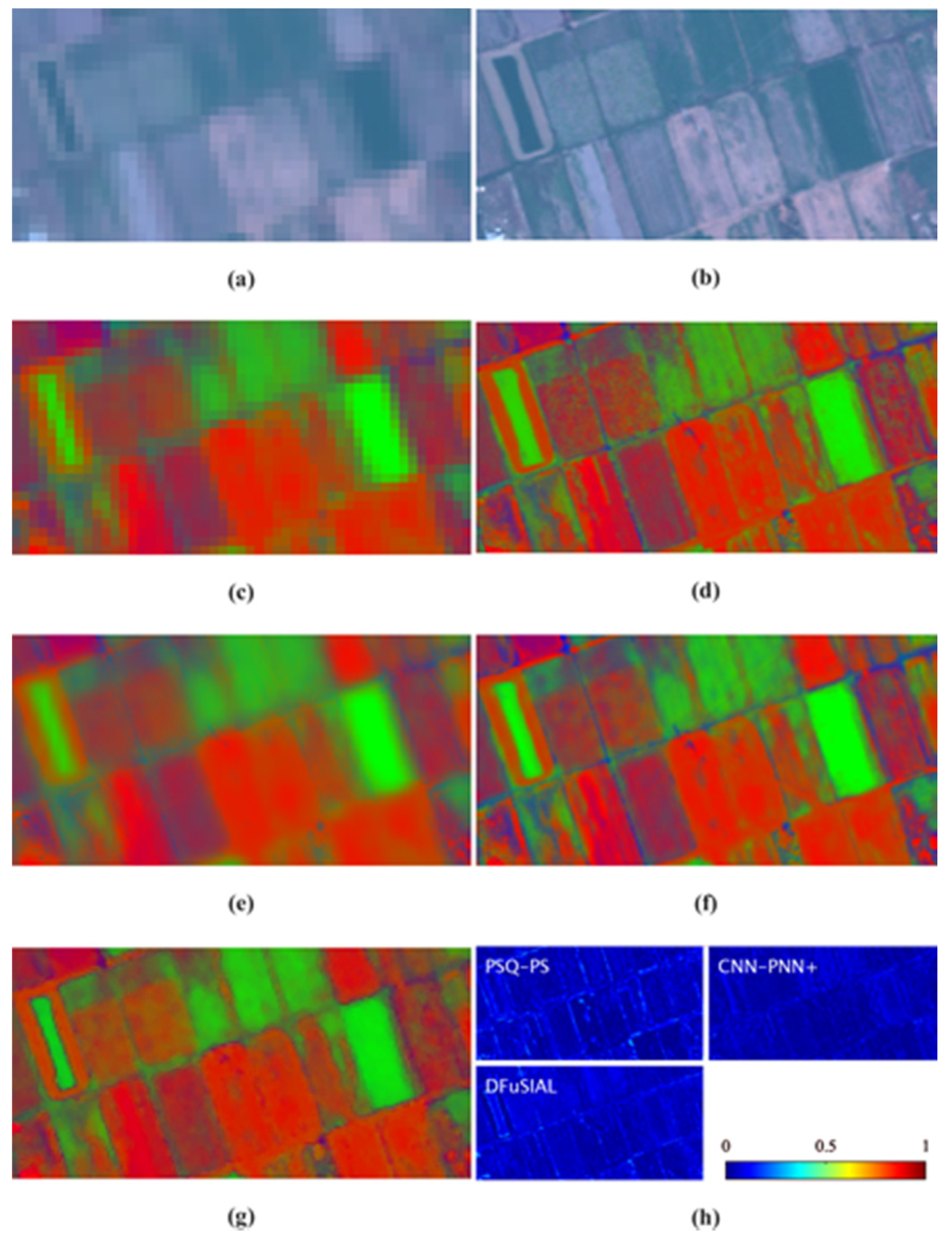
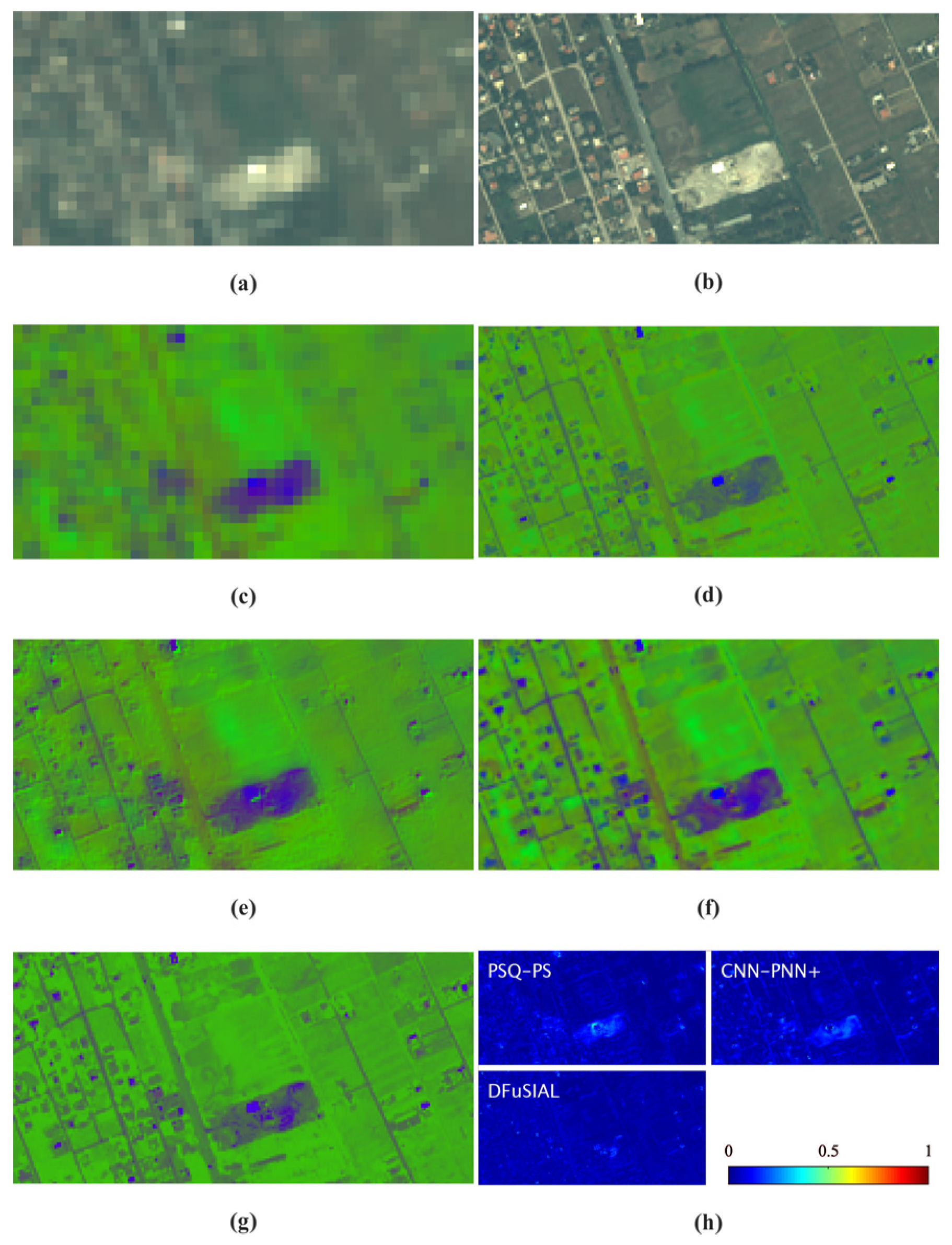
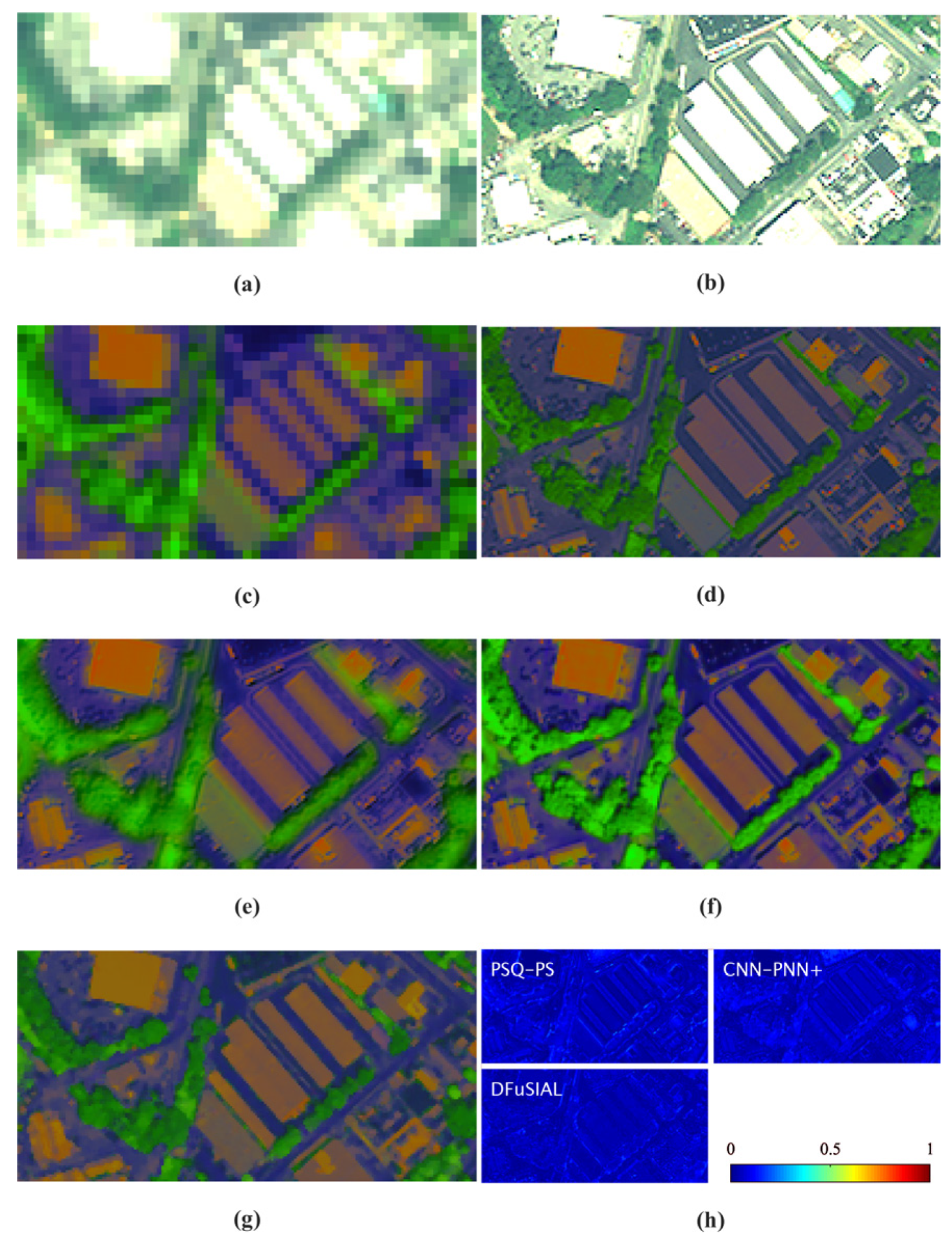
The conventional filter-based approach, presented in [61], is intended for preserving spectral quality (PSQ). For the sake of convenience, we use the term PSQ-PS to refer to this method in the rest of the paper.

(2)

The novel CNN-based approach, presented in [26], utilizes a target-adaptive fine-tuning step to achieve a further improvement of the results with comparison to its baseline and accurate method pansharpening neural network (PNN) [25]. We use the term CNN-PNN+ to refer to this method in the rest of the paper.

Since CNN-PNN+ is designed for particular types of data, it is used for comparison only in experiments that involve dataset from Group-2.

Four different experiments are performed to evaluate the performance of the proposed method and for comparison with the state-of-the-art PSQ-PS and CNN-PNN+. In each experiment, we use three evaluation metrics: the mean absolute error (MAE), the root mean square error (RMSE), and the maximal absolute error (MaxAE). Let $f_{i,j}$ and ${\widehat{f}}_{i,j}$ be, respectively, the reference and the estimated fraction values of the i-th EM in the j-th evaluation point. The absolute error (AE) and the square error (SE) of the estimated fraction ${\widehat{f}}_{i,j}$ are given by

$$\begin{array}{c}{\mathrm{AE}}_{i,j}=\left|f_{i,j}-{\widehat{f}}_{i,j}\right|\\ \mathrm{and}\\ {\mathrm{SE}}_{i,j}={\left(f_{i,j}-{\widehat{f}}_{i,j}\right)}^2.\end{array}$$

(7)

Let $q$ be the number of points to be used for the evaluation. The ${\mathrm{MAE}}_i$, its standard deviation (${\mathrm{STD}}_i$), the ${\mathrm{RMSE}}_i$ and the ${\mathrm{MaxAE}}_i$ for the i-th EM are computed as follows:

$$\begin{array}{c}{\mathrm{MAE}}_i=\raisebox{1ex}{$1$}\!\left/ \!\raisebox{-1ex}{$q$}\right.{\displaystyle \sum _{j=1}^q{\mathrm{AE}}_{i,j}},\\ {\mathrm{STD}}_i=\sqrt{\raisebox{1ex}{$1$}\!\left/ \!\raisebox{-1ex}{$q$}\right.{\displaystyle \sum _{j=1}^q{\left({\widehat{f}}_{i,j}-{\mathrm{MAE}}_i\right)}^2}},\\ {\mathrm{RMSE}}_i=\sqrt{\raisebox{1ex}{$1$}\!\left/ \!\raisebox{-1ex}{$q$}\right.{\displaystyle \sum _{j=1}^q{\mathrm{SE}}_{i,j}}},\\ \mathrm{and}\\ {\mathrm{MaxAE}}_i=\max \left\{{\mathrm{AE}}_{i,j}\right\}, j=1\dots q\end{array}$$

(8)

Then, the average $\mathrm{MAE}$, $\mathrm{STD}$, $\mathrm{RMSE}$, and $\mathrm{MaxAE}$ for the experimented image are given by;

$$\begin{array}{c}\mathrm{MAE}=\raisebox{1ex}{$1$}\!\left/ \!\raisebox{-1ex}{$d$}\right.{\displaystyle \sum _{i=1}^d{\mathrm{MAE}}_i},\\ \mathrm{STD}=\raisebox{1ex}{$1$}\!\left/ \!\raisebox{-1ex}{$d$}\right.{\displaystyle \sum _{i=1}^d{\mathrm{STD}}_i},\\ \mathrm{RMSE}=\raisebox{1ex}{$1$}\!\left/ \!\raisebox{-1ex}{$d$}\right.{\displaystyle \sum _{i=1}^d{\mathrm{RMSE}}_i},\\ \mathrm{and}\\ \mathrm{MaxAE}=\max \left\{{\mathrm{MaxAE}}_i\right\}, i=1\dots d\end{array}$$

(9)

where $d$ is the number of EMs. The following two types of evaluations are applied:

Type 1:

The $\mathrm{MAE}$, its $\mathrm{STD}$, the $\mathrm{RMSE}$, and the $\mathrm{MaxAE}$ values of the fractions obtained by the different methods are computed according to Equations (7)–(9), with respect to HSR ground truth (GT) fraction maps derived by applying SUnSAL on the available HSR spectral image. All pixels in the HSR are used in the evaluation.

Type 2:

The $\mathrm{MAE}$, its $\mathrm{STD}$, the $\mathrm{RMSE}$, and the $\mathrm{MaxAE}$ values are computed with respect to the fractions obtained by SUnSAL for the LSR spectral image. Only IPs are used in this evaluation. More specifically, we use 20% of IPs for the evaluation, and the rest (80%) are used to feed and train the SFANN.

1. Experiment 1: Testing with real full reference ground truth

In this experiment, we use the datasets from Group-1, i.e., sets 1, 2, and 3, to evaluate the performance of the tested methods under cases with images from different sensors, images from the same sensor, and images with missing data pixels. We perform four evaluation tests as follows:

● Test 1—data from different sensors, Landsat and Sentinel

In this test, we use the Landsat image with an LSR of 30 m and the visible bands of the Sentinel image to create a corresponding RGB image with an SR of 10 m. The SIFT method detected 2600 IPs. Figure 8 presents an RGB composite of the images used in this experiment with a plot of the extracted IPs.

● Test 2—data from the same sensor, Venus dataset-a

We use the Venus image from the second dataset with an SR of 10 m as an LSR spectral image and the visible bands of the corresponding image provided by the same satellite as an HSR RGB image with an SR of 5 m (Figure 6). The SIFT method detected 3560 IPs

● Test 3—data from the same sensor, Venus dataset-b

Like in Experiment 2, we apply the same test to the third dataset, which contains multiple homogeneous regions (Figure 6). The SIFT method detected 1790 IPs.

● Test 4—data from different sensors with simulated missing-data pixels.

Here we use the same data set as in Test 1. To simulate a case with missing data, we create vertical missing-data stripes across the LSR image (see Figure 9). We set the width of each stripe to five pixels and the distance between the stripes to 50 pixels. The SIFT method detected 500 IPs. Figure 9 presents an RGB composite of the images used in this experiment with a plot of the extracted IPs. It shows that IPs are detected only within a certain distance from missing data pixels. This property ensures the SFFAN is fed only with reliable data, which is essential for unbiased learning.

We use the available HSR spectral image to create an HSR reference fraction map to serve as the ground truth in each experiment. In Tests 1 and 4, we first spectrally convolve the bands of the Sentinel image to the spectral bands of the Landsat 8 image. We use the obtained results by applying SUnSAL to the HSR image as reference for the 1 ^st type of evaluation, whereas, for the 2 ^nd type, we use the LSR fraction maps as reference. In each of the four experiments, we apply the proposed DFuSIAL to enhance the SR of the obtained fraction maps for the LSR image and generate fraction maps with HSR. The PSQ-PS method is applied for comparison. First, we apply the PS process to retrieve the HSR spectral image. For this purpose, we use the LSR spectral image with a panchromatic image that we derive from the original HSR spectral image. Then, we obtain HSR fraction maps by applying SUnSAL to the retrieved HSR spectral image.

To test the stability of the solution under different SFFAN architectures, we experiment with a different number of hidden layers and neurons. In practice, we examine the performance of the DFuSIAL method using 15 different combinations. We apply different SFANNs with a varying number of hidden layers (3 to 5, i.e., $k=3,4 \mathrm{or} 5$) and a different number of neurons in each layer (by setting $c=10,20,30,40 \mathrm{or} 50$). Empirical tests reveal that all configurations yield quite similar results. Nevertheless, the two SFFANs with ($k=3$, $c=30$) and ($k=5$, $c=10$) were found to be optimal: they performed faster and minimized the MAE for the data sets used in this work. Six EMs which we automatically extracted from the spectral image using the VCA method were used in each of the experimental tests 1–4.

2. Experiment 2: Testing with simulated full reference ground truth and comparing with CNN-based PS method

We use the datasets from Group-1, i.e., sets 4,5, and 6, to perform three experimental tests as follows:

● Test 5—data from GeoEye-1 with simulated reference ground truth

In this test, we use the resampled GeoEye-1 image, from data set 4, with reduced LSR of 7.36 m and the visible bands of the original GeoEye-1 image to create a corresponding RGB image with an SR of 1.84 m. The SIFT method detected 98 IPs.

● Test 6—data from Ikonos with simulated reference ground truth

Like in Test 5, we use the resampled Ikonos image, from dataset 6, with reduced LSR of 13.12 m and the corresponding RGB bands from the original image with HSR of 3.28 m. The SIFT method detected 110 IPs.

● Test 7—data from WorlView-2 with simulated reference ground truth

Similar to Tests 3 and 4, we use the resampled WorldView-2 image, from dataset 6, with reduced LSR of 7.36 m and the corresponding RGB band from the original image with HSR of 1.84 m. The SIFT method detected 140 IPs.

In all of the tests, 5, 6, and 7, the original spectral image is used for generating reference ground truth. Since GeoEye-1 and Ikonos images have only four bands, the number of EMs which we automatically extracted using the VCA method in Tests 4 and 5 is three, whereas in Test 6 we use six EMs. Both PSQ-PS and CNN-PNN+ methods are applied for comparison in this experiment. Moreover, the number of detected IPs in these three tests was relatively low due to the small size of the images. Thus, we set the number of layers and neurons in the SFANN to three and ten, i.e., $k=3$ and $c=10$, respectively.

3. Experiment 3: Hierarchal resolution enhancement

● Test 8—We use the images from the seventh dataset; the Sentinel spectral image, with an SR of 10 m, an RGB image from Google Earth with an SR of 1 m, and an RGB image with an SR of 3 m that was created by resampling the 1 m RGB image. Six EMs extracted from the Sentinel image by VCA are used, and their fractions are estimated using SUnSAL. Then, we use a hierarchal DFuSIAL process to create fraction maps with SRs of 3 m and 1 m, as follows:

Step 1: Training the SFANN to estimate fractions for the RGB image, with an SR of 3 m, using the DFuSIAL algorithm.

Step 2: To further enhance the resolution of fraction maps, we first radiometrically calibrate the Google Earth RGB image of the same area but with an SR of 1 m. Then, we apply the trained SFANN to the calibrated image to obtain fraction maps with an SR of 1 m.

For comparison, we use the PS fusion method to create corresponding fraction maps as follows:

Step 1: The PSQ-PS method is applied to create a new multispectral image with an SR of 3 m by fusing the original Sentinel 10 m image and a panchromatic image created from the RGB 3 m image.

Step 2: Creating a new multispectral image with an SR of 1 m using the PSQ-PS method to fuse the multispectral 3 m image created in Step 1 and a panchromatic image created from the RGB 1 m image.

Step 3: Applying SUnSAL to the two multispectral images created in Steps 1 and 2 to generate fraction maps with SRs of 3 m and 1 m, respectively.

An RGB composite of the images and the corresponding fraction map of three selected EMs are presented in the Section 3.

4. Experiment 4: Testing the influence of rotation and displacement mismatch between data sources.

In this experiment, we test the robustness of the examined methods to probable rotation and displacement mismatch between the spectral and RGB images. For this purpose, we use the images from the seventh dataset, i.e., WorlView-2. A description of the experiment and interpretation of the results are given in the results and discussions, i.e., Section 3.

To minimize the influence of a probable difference in radiometric values, both the HSR and LSR spectral images need to be in reflectance units. For this purpose, robust radiometric empirical line calibration is applied in each experimental test to the HSR image with respect to the LSR spectral image, using the valid IPs.

Table 1. Summarized information about the data sources used in the experimental tests 1 to 8.

		Data Set	HSR Data	LSR Data	Number of Detected IPs	RISFL Parameters
						s	n
Experiment 1	Test 1	1	Sentinel-2 A SR = 10 m 900 × 1800 × 7 *	Landsat-8 SR = 30 m 300 × 600 × 7	1696	5 × 5	6
	Test 2	2	Venus SR = 5 m 800 × 1600 × 12 *	Venus SR = 10 m 400 × 800 × 12	3568	5 × 5	6
	Test 3	3	Venus SR = 5 m 800 × 1600 × 12 *	Venus SR = 10 m 400 × 800 × 12	1791	7 × 7	6
	Test 4	1	Sentinel-2 A SR = 10 m 900 × 1800 × 7 *	Landsat-8 SR = 30 m 300 × 600 × 7 With simulated missing-data pixels	499	5 × 5	6
Experiment 2	Test 5	4	GeoEye-1 SR = 1.84 m 320 × 320 × 4 *	Resampled GeoEye-1 SR = 7.36 m 80 × 80 × 4 *	98	5 × 5	4
	Test 6	5	Ikonos SR = 3.28 m 320 × 320 × 4 *	Resampled Ikonos SR = 13.12 m 80 × 80 × 4 *	110	5 × 5	4
	Test 7	6	WorldView-2 SR = 1.84 m 320 × 320 × 7 *	Resampled WorldView-2 SR = 7.36 m 80 × 80 × 7 *	140	5 × 5	4
Experiment 3	Test 8	7	Google Earth SR = 1 m 1975 × 2269 × 3 *	Sentinel-2 A SR = 10 m 213 × 245 × 7 *	200 **	5 × 5	4

Note: s = neighborhood size; n = number of directional regions; * number of rows x columns x spectral bands in image; ** the IPs are between the MS image and the resampled RGB image with SR = 3.

summarizes information about the data sources used in each experimental test. In all seven tests, we feed the network with 80% of the detected IPs and use the other 20% for evaluation type 2. Figure 10 shows an overview of the applied comparative testing used for the evaluation in experiments 1 and 2.

3. Results and Discussion

3.1. Quantitative Evaluation

To analyze the performance of the proposed method, DFuSIAL, and the other tested state-of-the-art methods, we observe both the quantitative and visual outcomes of the applied experiments.

Table 2. Type-1 evaluation of fraction values, obtained in Experiment 1 (Tests 1–4) by PSQ-PS and the proposed fusion method DFuSIAL, with respect to the obtained fractions, in HSR by SUnSAL.

Type-1 Evaluation
	PSQ-PS				DFuSIAL
	MAE	STD	RMSE	Max	MAE	STD	RMSE	Max
Test 1	0.035	0.046	0.058	0.172	0.033	0.038	0.051	0.148
Test 2	0.028	0.032	0.043	0.124	0.028	0.030	0.044	0.122
Test 3	0.019	0.027	0.031	0.096	0.029	0.042	0.056	0.133
Test 4	0.057	0.072	0.093	0.274	0.034	0.040	0.052	0.152

Notes: Bold font indicates best result for each evaluation metric.

and

Table 3. Type-2 evaluation of fraction values, obtained in Experiment 1 (Tests 1-4) by PSQ-PS and the proposed fusion method DFuSIAL, with respect to the obtained fractions, in LSR by SUnSAL.

Type-2 Evaluation
	PSQ-PS				DFuSIAL
	MAE	STD	RMSE	Max	MAE	STD	RMSE	Max
Test 1	0.024	0.034	0.043	0.126	0.022	0.031	0.043	0.121
Test 2	0.024	0.030	0.038	0.113	0.024	0.031	0.039	0.117
Test 3	0.015	0.021	0.026	0.074	0.020	0.025	0.029	0.080
Test 4	0.060	0.072	0.094	0.272	0.034	0.036	0.051	0.141

present the $\mathrm{MAE}$, $\mathrm{STD}$, $\mathrm{RMSE}$ and overall $\mathrm{MaxAE}$ values of Type 1 and Type 2 evaluations, respectively, for the obtained fractions in Experiment 1. The results show that both PSQ-PS and DFuSIAL provide reliable results, with an average $\mathrm{MAE}$ between 2% and 4%. Indeed, the performance of both methods is highly correlated, with the exception of Test 4. The results obtained by DFuSIAL in Test 1 are more accurate than those obtained by PS. This advantage is mainly due to the absence of full spatial and temporal overlapping between the LSR and HSR data sources. The IP-based aided learning in DFuSIAL minimizes the influence of this lack of overlapping.

On the other hand, the results obtained by the PSQ-PS method in Test 3 are even more accurate. As mentioned before, the images in this experiment mainly include homogeneous regions. Since the detection of IPs within these regions is challenging, the number of IPs detected is almost half the number detected in Test 1 for a dataset of the same size and from the same sensor (see Table 1 for information on Tests 2 and 3). The relative lack of IPs within homogeneous regions reduces the ability of the SFFAN to learn the relationship between the fractions and the RGB data in these areas.

Unlike the results of Tests 1–3, the results of Test 4 clearly show the advantage of DFuSIAL over PSQ-PS with respect to the accuracy of the fractions. The presence of missing-data pixels in the image has a tremendous negative influence on the PSQ-PS process, whereas IP-based learning prevents this influence. In practice, DFuSIAL is only slightly affected by missing-data pixels due to a lower number of detectable IPs (see Figure 9), and accordingly, fewer training data samples. With the exception of Test 3, $\mathrm{STD}$ and $\mathrm{MaxAE}$ values are lower for fractions obtained by DFuSIAL. The increase in $\mathrm{MaxAE}$ for the PSQ-PS method in Test 4 is noticeable, whereas the corresponding value for DFuSIAL is similar to that obtained in Test 1. This is due mainly to the robustness of the proposed method to missing-data pixels. In addition to the previous insights, the results show that $\mathrm{MAE}$, $\mathrm{STD}$, $\mathrm{RMSE}$ and $\mathrm{MaxAE}$ values obtained using evaluation types 1 and 2 are correlated and so type-2 evaluation may be used as an efficient indicator of process accuracy. This fact is beneficial in real cases, where a reference ground truth of the HSR fraction maps is not available for validation purposes.

In the same context,

Table 4. Type-1 evaluation of fraction values, obtained in Experiment 2 (Tests 5–7) by PSQ-PS, CNN-PNN+, and the proposed fusion method DFuSIAL, with respect to the obtained fractions, in HSR by SUnSAL.

Type-1 Evaluation
	PSQ-PS				CNN-PNN+				DFuSIAL
	MAE	STD	RMSE	Max	MAE	STD	RMSE	Max	MAE	STD	RMSE	Max
Test 5	0.051	0.055	0.075	0.215	0.038	0.037	0.053	0.150	0.055	0.050	0.075	0.209
Test 6	0.040	0.041	0.058	0.164	0.041	0.039	0.056	0.157	0.034	0.027	0.044	0.116
Test 7	0.063	0.069	0.095	0.270	0.059	0.065	0.090	0.254	0.050	0.040	0.064	0.170

Notes: Bold font indicates best result for each evaluation metric.

presents the $\mathrm{MAE}$, $\mathrm{STD}$, $\mathrm{RMSE}$, and overall $\mathrm{MaxAE}$ values of Type 1 and Type 2 evaluations, respectively, for the obtained fractions in Experiment 2, i.e., Tests 5–7. As mentioned before, in this experiment, both the methods PSQ-PS and CNN-PNN+ are used for comparison. The results in Table 4 clearly show the advantage of the proposed DFuSIAL over the two other methods in Tests 6 and 7, with respect to all the metrics used for the evaluation. On the other hand, the obtained results by CNN-PNN+ in Test 5 are the most accurate among the three tested methods. Besides, PSQ-PS slightly outperforms DFuSIAL in this test. In accordance with the results from Test 3 in Experiment 1, the results in Test 5 point out the slight increase of the $\mathrm{MAE}$ of the obtained results by DFuSIAL for images with a high presence of homogenous regions.

In Experiment 3 (Test 8), since HSR reference fraction maps are not available, we apply only the 2^nd type of evaluation (see

Table 5. Average values obtained by evaluation type 2 of HRS fraction values obtained in Experiment 3 (Test 8) by PSQ-PS and the proposed fusion method DFuSIAL, with respect to the LSR fractions obtained by SUnSAL.

Evaluation Type 2
	PSQ-PS				DFuSIAL
	MAE	STD	RMSE	Max	MAE	STD	RMSE	Max
Test 8	0.078	0.101	0.128	0.353	0.043	0.050	0.065	0.172

Notes: Bold font indicates best result for each evaluation metric.

). The enhanced-resolution fractions obtained by DFuSIAL have an average MAE of ~4.5%. The error for all evaluation metrics is slightly increased, compared with previous experiments, mainly due to changes in the land cover types between the two data sources that were acquired more than three years apart. Nonetheless, objects with invariant land cover, e.g., roofs, are assumed to preserve their fraction values, as shown later in the visual presentation of the results. On the other hand, the PSQ-PS method is highly influenced not only by temporal changes but also by the lack of overlap between the images. Thus, the fractions obtained by the PSQ-PS method have an average MAE of ~8% and a significantly increased error for all of the evaluation metrics used.

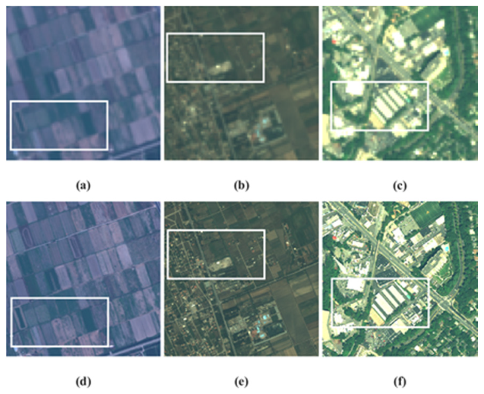
3.2. Visual Evaluation

To facilitate a visual evaluation, we present the fraction maps and MAE maps obtained in each experiment. Specifically, we present a combination of the fraction maps of three of the EMs used in the experiment. For each scenario, we select three dominant EMs, denoted EM1, EM2, and EM3. We then generate a false color composite by using the fraction maps of the three EMs as R, G, and B layers, respectively and use a color pyramid to interpret the obtained false color maps. Vertices (1,0,0), (0,1,0), and (0,0,1) are red, green, and blue, respectively, and represent pure pixels of EM1, EM2, and EM3, respectively. The points on the triangular face created by these three vertices represent pixels with different mixtures of the three selected EMs. Vertex (0,0,0) is black and represents a pixel with a mixture of the other EMs and a fraction value of zero for each of the three selected EMs. Other points located within the pyramid volume and on the triangular faces connected to vertex (0,0,0), represent different mixtures of different combinations of the six EMs. Figure 11 presents the planar unfolding of the color pyramid. Figure 12, Figure 13, Figure 14 and Figure 15 present a zoom-in of selected areas of the fraction maps obtained in Experiment 1, i.e., Tests 1–4, respectively, by applying SUnSAL to the original LSR and HSR spectral images and by using the PSQ-PS method and the proposed DFuSIAL. Similarly, Figure 16, Figure 17 and Figure 18 present the obtained maps by PSQ-PS, CNN-PNN+, and DFuSIAL in Experiment 2, i.e., Tests 5–7. Besides, in Experiment 1, we present the entire error map for each of the tested methods, while in Experiment 2, due to size limitation, we present only a part of the MAE maps that corresponds to the selected area for presentation in each test. We derive the error map by calculating the MAE of the fraction value obtained for each pixel with respect to the GT fractions obtained by applying SUnSAL to the available HSR spectral image. An independent color bar is attached to the MAE maps in each figure to facilitate interpretation of the MAE values.

The visual presentation of the results in Experiment 1 clearly shows the enhancement of fraction map resolution achieved by both methods. Figure 12 shows the advantage of DFuSIAL over the PSQ-PS method, which is in line with our quantitative results. This advantage is especially noticeable in areas in which the fractions undergo rapid spatial changes, e.g., the area containing roofs. Although both methods introduce specific spatial regularization into the estimated fractions, the results obtained by PSQ-PS are oversmoothed, and small spatial features are filtered out of the obtained fraction map. This spatial regularization is controlled in DFuSIAL mainly by changing the parameters used for RISFL extraction. The results presented for Tests 2 and 3 (see Figure 13 and Figure 14, respectively) show a high correlation between the results obtained by the two methods. It is essential to mention that this correlation holds for both the spatial distribution and the intensity of the fractions, which means that the obtained fraction values are highly similar. The MAE maps in Figure 14 emphasize the advantage of the PSQ-PS method over DFuSIAL within homogeneous regions, although DFuSIAL performs better along the boundaries between these regions. The results presented in Figure 15 are essential and show the significant advantage of DFuSIAL in cases that contain missing-data pixels. While the presence of such pixels has a clear negative influence on the results obtained by the PSQ-PS method, the results obtained by DFuSIAL are not affected. As can be observed in Figure 15b, the PSQ-PS method retrieves only a minor amount of information from the missing-data stripes, yet the footprint of these stripes appears clearly in both fraction and MAE maps. On the other hand, the results obtained by DFuSIAL are similar to those obtained in Test 1, without missing-data pixels, indicating high robustness of the proposed fusion method to this kind of influence.

Similar to the insights from Experiment 1, the visual presentation of the results in Experiment 2 emphasizes the achieved enhancement of fraction map by the three examined methods. Moreover, and in accordance with the quantitative results, the visual interpretation of the results shows that except for the case with the high presence of homogeneous areas, DFuSIAL has a significant advantage over the other two examined methods. The maps in Figure 16, Figure 17 and Figure 18 clearly show that while the obtained results by CNN-PNN+ and DFuSIAL preserve the sharpness of the fraction maps, to a high extent, the obtained maps by PSQ-PS are significantly oversmoothed. This probably occurs due to the use of a filter-based approach. Moreover, while the obtained maps by CNN-PNN+ look more similar to the reference fractions, with regards to their spatial distribution, the obtained fractions by DFuSIAL are more accurate with regards to their real value. For example, the results in Figure 18 clearly show that there is an overestimation of the vegetation EM within the obtained fractions by CNN-PNN+.

Regarding experiment 3 (Test 8), the results clearly show the ability of the DFuSIAL method to significantly enhance the SR of the fraction maps also through a hierarchical process. The obtained results, of both 3 m and 1 m resolutions, preserve the sparsity of the fractions. The trained SFANN is very useful for further enhancing the resolution. In this case, the resampled image, with a 3 m resolution, is used as a mediator in the process to enhance the resolution from 10 m to 1 m. In practice, once a SFANN is created and trained according to the DFuSIAL algorithm, the trained network can be applied to different images from the same area but with different resolutions.

On the other hand, due to the lack of full overlap between the multispectral and the RGB images, the geometrical distortion is noticeable in the results obtained by the PSQ-PS method. In this regard, the results presented in Figure 19 emphasize the robustness of DFuSIAL to temporal and geometrical partial-nonoverlapping between the fused data sources. It is important to note that direct enhancement, from a 10 m to a 1 m resolution, yielded quite similar results to those obtained by the described hierarchal process. The hierarchal process is, however, more efficient in terms of computation time and complexity.

In summary, both the quantitative and visual results in Experiments 1–3 show that DFuSIAL is preferable not only for cases with data from different sensors but also for data from the same sensor and when the SR of the RGB image is significantly larger than that of the spectral image used for the fusion. While the effort in other fusion methods is to retrieve the entire HSR MS image, the focus in DFuSIAL is only on enhancing the SR of one product of the spectral data, i.e., the EM fractions. The pattern that DFuSIAL needs to learn is, therefore, more straightforward and relatively less complicated. Thus, it outperforms the other examined methods with regards to the accuracy of the spatially enhanced fraction maps. On the other hand, the performance of DFuSIAL is slightly affected by the presence of homogeneous areas within the fused image, since fewer IPs are detected within these areas.

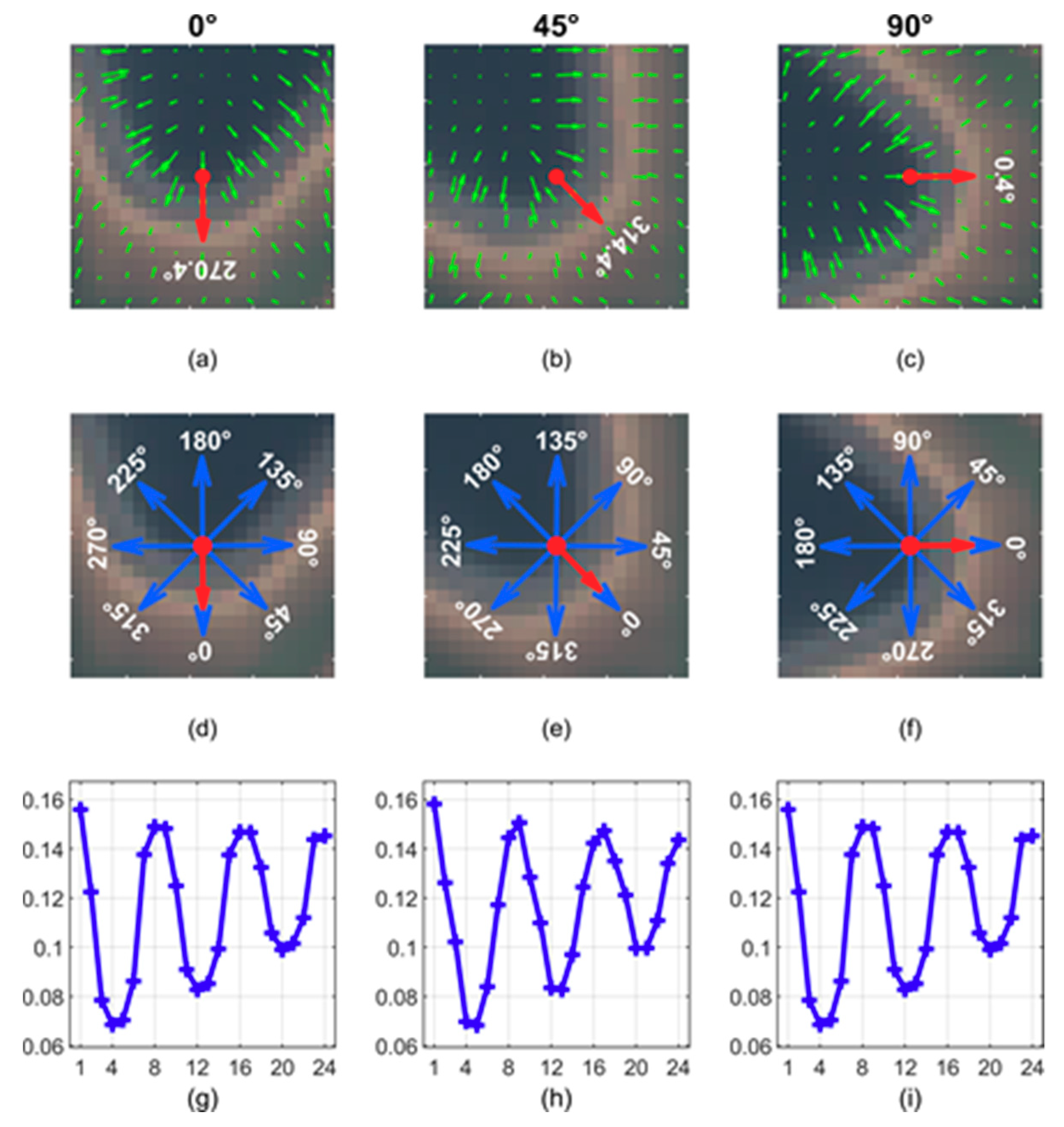
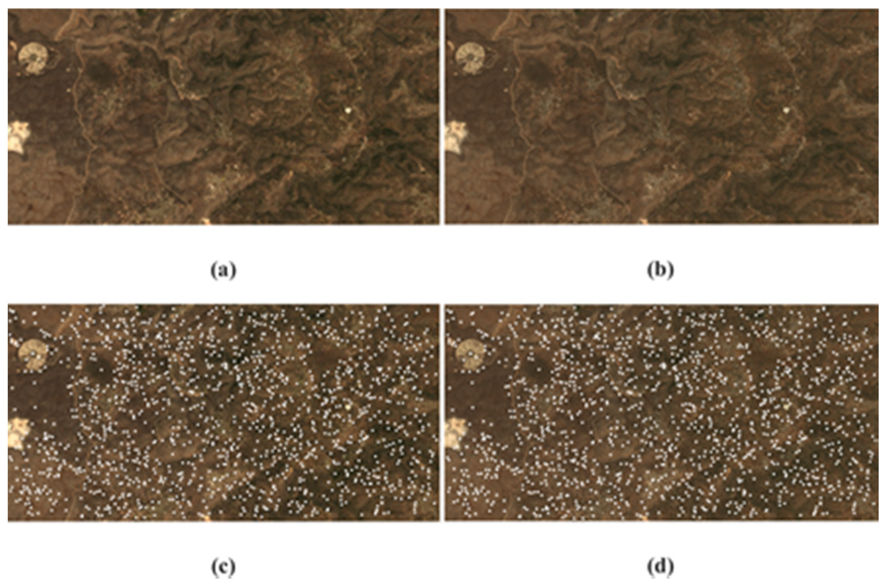
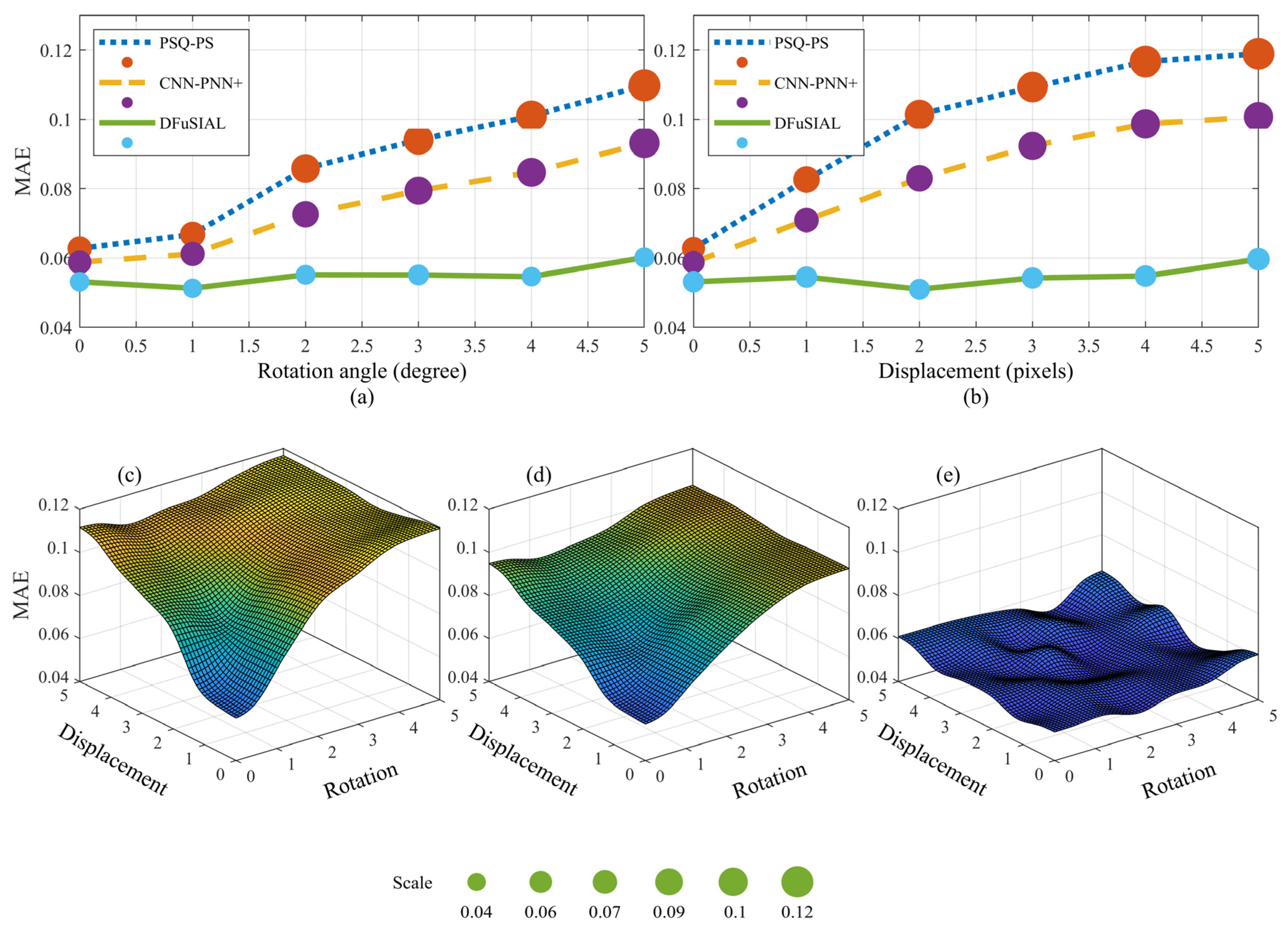
3.3. Evaluation of the Performance under Rotation and Displacement Mismatch between Data Sources (Experiment 4)

The results of Tests 1, 4, and 8 demonstrate the advantage of using DFuSIAL to fuse data from different sources. This advantage is due mainly to the robustness of DFuSIAL to mismatches between the images. Although the mismatch between the Landsat and Sentinel images is relatively minor, it nevertheless affects the PSQ-PS method negatively. In many cases, especially when using modern remote sensing platforms, e.g., unmanned aerial vehicles, this mismatch can reach considerable proportions. Thus, to test the robustness of the PSQ-PS, CNN-PNN+, and DFuSIAL methods under significant mismatch conditions, we repeat Test 7 while creating a gradual mismatch between the data sources, i.e., the original WorldView-2 image and its corresponding resampled image with reduced SR. First, we create pairs of data with different degrees of radial and displacement mismatch by rotating the LSR image at an angle of $0°,1°,2°,3°,4°, \mathrm{and} 5°$ and shifting the HSR image by 0, 1, 2, 3, 4, and 5 pixels. In each of the 36 combinations, we fuse the images using the three methods and observe the MAE value and its standard deviation, as explained previously (see Figure 20).

Figure 20 clearly shows the superiority of the DFuSIAL method over the PSQ-PS and CNN-PNN+ methods with regards to the accuracy of the retrieved HSR fraction maps. DFuSIAL is robust to the two examined types of data source mismatch. In contrast, the MAE and STD values according to the PSQ-PS CNN-PNN+ methods increase rapidly and monotonously with the increase in mismatch. The use of IPs for learning and the incorporation of spatial information through invariant features, i.e., RISFLs, make the proposed method DFuSIAL highly robust to mismatches between the data sources. Thus, it is more suitable for the fusion of data from different instruments.

3.4. Sensitivity Test

The results obtained by DFuSIAL are sensitive mainly to two flexible parameters of the SFANN: (a) number of layers and (b) number of neurons in each layer. To test this sensitivity, we repeat the fusion process with 25 different combinations of these two parameters. We set the number of layers to 1, 2, 3, 4, or 5, and the number of neurons to 10, 15, 20, 25, or 30. In each case, we apply the fusion process and examine the performance of the method by observing the MAE of the results and the run time of the network training. We repeat the test ten times, picking the median values to prevent the influence of unexpected events during the calculations (see Figure 21). MAE values vary from 0.054 to 0.057, with a moderate variance. The MAE surface shows that increasing the number of layers in the network decreases the magnitude of the error more than doubling the number of neurons in each layer. In terms of computation run time, increasing the number of layers or the number of neurons increases the run time quadratically. Besides, the number of extracted IPs limits the allowed number of layers and neurons in the network. Thus, we should test these two parameters carefully when designing a new SFANN.

Table 6. Run time (sec) for PSQ-PS and the proposed fusion method DFuSIAL in Tests 1-4.

	PSQ-PS	DFuSIAL
	Runtime (s)	Runtime (s)
Test 1	65	90
Test 2	70	193
Test 3	74	76
Test 4	65	79

shows the computation run time of the methods in each test in Experiment 1. The overall run time of PSQ-PS for fraction estimation includes two main parts: (a) retrieval of an HSR spectral image, and (b) fraction estimation through unmixing. On average, the first part requires 60% of the computation run time, while the second part requires 40%. In DFuSIAL, the overall process includes four parts: (a) unmixing of the LSR spectral image, (b) extraction of IPs and empirical line calibration, (c) RISFL extraction, and (d) training and application of the SFANN. On average, the respective percentages of the total computation run-time are ~5%, 15%, 20%, and 60%.

4. Conclusions

Traditional methods for spectral unmixing rely only on spectral images. On the other hand, image fusion methods usually require datasets form the same sensor and that overlap both geometrically and temporally. Addressing these two limitations, we developed a new methodology for enhancing the SR of the fraction maps through data fusion of HSR visible images and LSR spectral images. Using automatically extracted IPs for learning, the proposed DFuSIAL is highly robust to the geometrical and acquisition conditions and to changes due to different acquisition dates. It is, therefore, beneficial for the fusion of data from different remote sensing instruments. Furthermore, we present a useful way for the incorporation of spatial information within NN-based learning, through RISFLs, without the need for CNNs. The results of real data experiments suggest that DFuSIAL gives both reliable and accurate results with respect to the HSR GT fraction maps. Comprehensive testing was applied using real data sets. A quantitative and visual evaluation of the results, with respect to two of the state-of-the-art conventional and CNN-based PS methods, shows that the proposed fusion method DFuSIAL is advantageous concerning the accuracy of the obtained HSR fraction maps. Furthermore, the proposed method was shown to be highly robust to an extreme mismatch between the fused data sources. It also yields a tenfold resolution enhancement by applying the hierarchal process. It would be interesting in future work to examine longer chains of the hierarchal process for further improvement as well as the use of additional metrics of the spatial features. Finally, the proposed framework is based on supervised learning through reliable IPs. In practice, once the input and output data samples are defined, other multivariate regression procedures, e.g., support vector machine [62] and random forest [63] (for regression), can be easily applied for the learning part of DFuSIAL and would also be considered in future work. Meanwhile, we prefer to use an FFNN for this purpose as it requires only a minimal number of assumptions and heuristic parameters.

References

1. Boreman, G.D. Classification of imaging spectrometers for remote sensing applications. Opt. Eng. 2005, 44, 013602. [Google Scholar] [CrossRef] [Green Version]
2. Garini, Y.; Young, I.T.; McNamara, G. Spectral imaging: Principles and applications. Cytom. Part. A 2006, 69, 735–747. [Google Scholar] [CrossRef]
3. Goetz, A.F.; Vane, G.; Solomon, J.E.; Rock, B.N. Imaging spectrometry for Earth remote sensing. Science 1985, 228, 1147–1153. [Google Scholar] [CrossRef] [PubMed]
4. Gat, N.; Subramanian, S.; Barhen, J.; Toomarian, N. Spectral imaging applications: Remote sensing, environmental monitoring, medicine, military operations, factory automation, and manufacturing. In Proceedings of the 25th Annual AIPR Workshop on Emerging Applications of Computer Vision, Washington, DC, USA, 26 February 1997; Volume 2962, pp. 63–77. [Google Scholar]
5. Manolakis, D.; Shaw, G. Detection algorithms for hyperspectral imaging applications. IEEE Signal. Process. Mag. 2002, 19, 29–43. [Google Scholar] [CrossRef]
6. Shaw, G.A.; Burke, H.K. Spectral imaging for remote sensing. Linc. Lab. J. 2003, 14, 3–28. [Google Scholar]
7. Klein, M.; Aalderink, B.; Padoan, R.; De Bruin, G.; Steemers, T. Quantitative hyperspectral reflectance imaging. Sensors 2008, 8, 5576–5618. [Google Scholar] [CrossRef] [Green Version]
8. Bioucas-Dias, J.M.; Plaza, A.; Dobigeon, N.; Parente, M.; Du, Q.; Gader, P.; Chanussot, J. Hyperspectral unmixing overview: Geometrical, statistical, and sparse regression-based approaches. IEEE J. Sel. Top. Appl. Earth Obs. Remote Sens. 2012, 5, 354–379. [Google Scholar] [CrossRef] [Green Version]
9. Li, W. Mapping urban impervious surfaces by using spectral mixture analysis and spectral indices. Remote Sens. 2020, 12, 94. [Google Scholar] [CrossRef] [Green Version]
10. Loncan, L.; De Almeida, L.B.; Bioucas-Dias, J.M.; Briottet, X.; Chanussot, J.; Dobigeon, N.; Fabre, S.; Liao, W.; Licciardi, G.A.; Simões, M.; et al. Hyperspectral pansharpening: A review. IEEE Geosci. Remote Sens. Mag. 2015, 3, 27–46. [Google Scholar] [CrossRef] [Green Version]
11. Meng, X.; Shen, H.; Li, H.; Zhang, L.; Fu, R. Review of the pansharpening methods for remote sensing images based on the idea of meta-analysis: Practical discussion and challenges. Inf. Fusion 2019, 46, 102–113. [Google Scholar] [CrossRef]
12. Yuan, Q.; Wei, Y.; Meng, X.; Shen, H.; Zhang, L. A multiscale and multidepth convolutional neural network for remote sensing imagery pan-sharpening. IEEE J. Sel. Top. Appl. Earth Obs. Remote Sens. 2018, 11, 978–989. [Google Scholar] [CrossRef] [Green Version]
13. Choi, J.; Yu, K.; Kim, Y. A new adaptive component-substitution-based satellite image fusion by using partial replacement. IEEE Trans. Geosci. Remote Sens. 2011, 49, 295–309. [Google Scholar] [CrossRef]
14. Nunez, J.; Otazu, X.; Fors, O.; Prades, A.; Pala, V.; Arbiol, R. Multiresolution-based image fusion with additive wavelet decomposition. IEEE Trans. Geosci. Remote Sens. 1999, 37, 1204–1211. [Google Scholar] [CrossRef] [Green Version]
15. Amolins, K.; Zhang, Y.; Dare, P. Wavelet based image fusion techniques—An introduction, review and comparison. ISPRS J. Photogramm. Remote Sens. 2007, 62, 249–263. [Google Scholar] [CrossRef]
16. Palsson, F.; Sveinsson, J.R.; Ulfarsson, M.O. A new pansharpening algorithm based on total variation. IEEE Geosci. Remote Sens. Lett. 2014, 11, 318–322. [Google Scholar] [CrossRef]
17. Yadaiah, N.; Singh, L.; Bapi, R.S.; Rao, V.S.; Deekshatulu, B.L.; Negi, A. Multisensor data fusion using neural networks. In Proceedings of the 2006 IEEE International Joint Conference on Neural Network Proceedings, Vancouver, BC, Canada, 16–21 July 2006. [Google Scholar]
18. Huang, W.; Xiao, L.; Wei, Z.; Liu, H.; Tang, S. A new pan-sharpening method with deep neural networks. IEEE Geosci. Remote Sens. Lett. 2015, 12, 1037–1041. [Google Scholar] [CrossRef]
19. Yang, J.; Fu, X.; Hu, Y.; Huang, Y.; Ding, X.; Paisley, J. PanNet: A deep network architecture for pan-sharpening. In Proceedings of the 2017 IEEE International Conference on Computer Vision (ICCV), Washington, DC, USA, 14–19 June 2017; pp. 1753–1761. [Google Scholar]
20. Palsson, F.; Sveinsson, J.R.; Ulfarsson, M.O. Multispectral and hyperspectral image fusion using a 3-D-convolutional neural network. IEEE Geosci. Remote Sens. Lett. 2017, 14, 639–643. [Google Scholar] [CrossRef]
21. Xing, Y.; Wang, M.; Yang, S.; Jiao, L. Pan-sharpening via deep metric learning. ISPRS J. Photogramm. Remote Sens. 2018, 145, 165–183. [Google Scholar] [CrossRef]
22. Ye, F.; Guo, Y.; Zhuang, P. Pan-sharpening via a gradient-based deep network prior. Signal. Process. Image Commun. 2019, 74, 322–331. [Google Scholar] [CrossRef]
23. Guo, P.; Zhuang, P.; Guo, Y. Bayesian Pan-Sharpening With Multiorder Gradient-Based Deep Network Constraints. IEEE J. Sel. Top. Appl. Earth Obs. Remote Sens. 2020, 13, 950–962. [Google Scholar] [CrossRef]
24. He, L.; Rao, Y.; Li, J.; Chanussot, J.; Plaza, A.; Zhu, J.; Li, B. Pansharpening via detail injection based convolutional neural networks. IEEE J. Sel. Top. Appl. Earth Obs. Remote Sens. 2019, 12, 1188–1204. [Google Scholar] [CrossRef] [Green Version]
25. Masi, G.; Cozzolino, D.; Verdoliva, L.; Scarpa, G. Pansharpening by convolutional neural networks. Remote Sens. 2016, 8, 594. [Google Scholar] [CrossRef] [Green Version]
26. Scarpa, G.; Vitale, S.; Cozzolino, D. Target-adaptive CNN-based pansharpening. IEEE Trans. Geosci. Remote Sens. 2018, 56, 5443–5457. [Google Scholar] [CrossRef] [Green Version]
27. Li, Z.; Cheng, C. A CNN-based pan-sharpening method for integrating panchromatic and multispectral images using landsat 8. Remote Sens. 2019, 11, 2606. [Google Scholar] [CrossRef] [Green Version]
28. Vitale, S.; Scarpa, G. A detail-preserving cross-scale learning strategy for CNN-based pansharpening. Remote Sens. 2020, 12, 348. [Google Scholar] [CrossRef] [Green Version]
29. Yang, Y.; Tu, W.; Huang, S.; Lu, H. PCDRN: Progressive cascade deep residual network for pansharpening. Remote Sens. 2020, 12, 676. [Google Scholar] [CrossRef] [Green Version]
30. Hinton, G.E.; Osindero, S.; Teh, Y.-W. A fast learning algorithm for deep belief nets. Neural Comput. 2006, 18, 1527–1554. [Google Scholar] [CrossRef]
31. Goh, G.B.; Hodas, N.O.; Vishnu, A. Deep learning for computational chemistry. J. Comput. Chem. 2017, 38, 1291–1307. [Google Scholar] [CrossRef] [Green Version]
32. Wang, D.; Li, Y.; Ma, L.; Bai, Z.; Chan, J. Going deeper with densely connected convolutional neural networks for multispectral pansharpening. Remote Sens. 2019, 11, 2608. [Google Scholar] [CrossRef] [Green Version]
33. Aiazzi, B.; Alparone, L.; Baronti, S.; Carla, R.; Garzelli, A.; Santurri, L. Sensitivity of pansharpening methods to temporal and instrumental changes between multispectral and panchromatic data sets. IEEE Trans. Geosci. Remote Sens. 2017, 55, 308–319. [Google Scholar] [CrossRef]
34. Mazzia, V.; Khaliq, A.; Chiaberge, M. Improvement in land cover and crop classification based on temporal features learning from sentinel-2 data using recurrent-convolutional neural network (R.-CNN). Appl. Sci. 2019, 10, 238. [Google Scholar] [CrossRef] [Green Version]
35. Lowe, D.G. Distinctive image features from scale-invariant keypoints. Int. J. Comput. Vis. 2004, 60, 91–110. [Google Scholar] [CrossRef]
36. Markham, B.L.; Storey, J.C.; Williams, D.L.; Irons, J.R. Landsat sensor performance: History and current status. IEEE Trans. Geosci. Remote Sens. 2004, 42, 2691–2694. [Google Scholar] [CrossRef]
37. Chang, C.I. Constrained subpixel target detection for remotely sensed imagery. IEEE Trans. Geosci. Remote Sens. 2000, 38, 1144–1159. [Google Scholar] [CrossRef] [Green Version]
38. Kizel, F.; Shoshany, M.; Netanyahu, N.S.; Even-Tzur, G.; Benediktsson, J.A. A stepwise analytical projected gradient descent search for hyperspectral unmixing and its code vectorization. IEEE Trans. Geosci. Remote Sens. 2017, 55, 4925–4943. [Google Scholar] [CrossRef]
39. Netanyahu, N.S.; Goldshlager, N.; Jarmer, T.; Even-Tzur, G.; Shoshany, M.; Kizel, F. An iterative search in end-member fraction space for spectral unmixing. IEEE Geosci. Remote Sens. Lett. 2011, 8, 706–709. [Google Scholar]
40. Iordache, M.-D.; Bioucas-Dias, J.M.; Plaza, A. Sparse unmixing of hyperspectral data. IEEE Trans. Geosci. Remote Sens. 2011, 49, 2014–2039. [Google Scholar] [CrossRef] [Green Version]
41. Shi, C.; Wang, L. Incorporating spatial information in spectral unmixing: A review. Remote Sens. Environ. 2014, 149, 70–87. [Google Scholar] [CrossRef]
42. Plaza, A.; Martinez, P.; Perez, R.; Plaza, J. A quantitative and comparative analysis of endmember extraction algorithms from hyperspectral data. IEEE Trans. Geosci. Remote Sens. 2004, 42, 650–663. [Google Scholar] [CrossRef]
43. Gao, G.; Gu, Y. Multitemporal landsat missing data recovery based on tempo-spectral angle model. IEEE Trans. Geosci. Remote Sens. 2017, 55, 3656–3668. [Google Scholar] [CrossRef]
44. Zhang, Q.; Yuan, Q.; Zeng, C.; Li, X.; Wei, Y. Missing data reconstruction in remote sensing image with a unified spatial–temporal–spectral deep convolutional neural network. IEEE Trans. Geosci. Remote Sens. 2018, 56, 4274–4288. [Google Scholar] [CrossRef] [Green Version]
45. Fischler, M.A.; Bolles, R.C. Random sample consensus. Commun. ACM 1981, 24, 381–395. [Google Scholar] [CrossRef]
46. Kizel, F.; Benediktsson, J.A. Data fusion of spectral and visible images for resolution enhancement of fraction maps through neural network and spatial statistical features. In Proceedings of the 9th Workshop on Hyperspectral Image and Signal Processing: Evolution in Remote Sensing (WHISPERS), Amsterdam, The Netherlands, 23–26 September 2018. [Google Scholar]
47. Bay, H.; Tuytelaars, T.; Van Gool, L. SURF: Speeded Up Robust Features; Springer: Berlin/Heidelberg, Germany, 2006; pp. 404–417. [Google Scholar]
48. Leutenegger, S.; Chli, M.; Siegwart, R.Y. BRISK: Binary Robust invariant scalable keypoints. In Proceedings of the IEEE International Conference on Computer Vision, Barcelona, Spain, 6–13 November 2011. [Google Scholar]
49. Kizel, F.; Shoshany, M. Spatially adaptive hyperspectral unmixing through endmembers analytical localization based on sums of anisotropic 2 D. Gaussians. Isprs J. Photogramm. Remote Sens. 2018, 141, 185–207. [Google Scholar] [CrossRef]
50. Smith, G.M.; Milton, E.J. The use of the empirical line method to calibrate remotely sensed data to reflectance. Int. J. Remote Sens. 1999, 20, 2653–2662. [Google Scholar] [CrossRef]
51. Kizel, F.; Benediktsson, J.A.; Bruzzone, L.; Pedersen, G.B.M.; Vilmundardottir, O.K.; Falco, N. Simultaneous and constrained calibration of multiple hyperspectral images through a new generalized empirical line model. IEEE J. Sel. Top. Appl. Earth Obs. Remote Sens. 2018, 11, 2047–2058. [Google Scholar] [CrossRef]
52. Svozil, D.; Kvasnicka, V.; Pospichal, J. Introduction to multi-layer feed-forward neural networks. Chemom. Intell. Lab. Syst. 1997, 39, 43–62. [Google Scholar] [CrossRef]
53. Hagan, M.T.; Menhaj, M.B. Training feedforward networks with the Marquardt algorithm. IEEE Trans. Neural Netw. 1994, 5, 989–993. [Google Scholar] [CrossRef]
54. Zhao, G.; Ahonen, T.; Matas, J.; Pietikainen, M. Rotation-invariant image and video description with local binary pattern features. IEEE Trans. Image Process. 2012, 21, 1465–1477. [Google Scholar] [CrossRef]
55. Dalal, N.; Triggs, B. Histograms of oriented gradients for human detection. In Proceedings of the 2005 IEEE Computer Society Conference on Computer Vision and Pattern Recognition (CVPR’05), San Diego, CA, USA, 20–25 June 2005; Volume 1, pp. 886–893. [Google Scholar]
56. Chen, Y.; Ye, X. Projection onto a simplex. arXiv 2011, arXiv:1101.6081. [Google Scholar]
57. Khoshsokhan, S.; Rajabi, R.; Zayyani, H. Sparsity-constrained distributed unmixing of hyperspectral data. IEEE J. Sel. Top. Appl. Earth Obs. Remote Sens. 2019, 12, 1279–1288. [Google Scholar] [CrossRef] [Green Version]
58. Nascimento, J.M.P.; Dias, J.M.B. Vertex component analysis: A fast algorithm to unmix hyperspectral data. IEEE Trans. Geosci. Remote Sens. 2005, 43, 898–910. [Google Scholar] [CrossRef] [Green Version]
59. Bioucas-Dias, J.M.; Figueiredo, M.A.T. Alternating direction algorithms for constrained sparse regression: Application to hyperspectral unmixing. In Proceedings of the 2nd Workshop on Hyperspectral Image and Signal Processing: Evolution in Remote Sensing, Reykjavik, Iceland, 4–16 June 2010. [Google Scholar]
60. Wald, L.; Ranchin, T.; Mangolini, M. Fusion of satellite images of different spatial resolutions: Assessing the quality of resulting images. Photogramm. Eng. Remote Sens. 1997, 63, 691–699. [Google Scholar]
61. Shahdoosti, H.R.; Ghassemian, H. Fusion of MS and PAN images preserving spectral quality. IEEE Geosci. Remote Sens. Lett. 2015, 12, 611–615. [Google Scholar] [CrossRef]
62. Peng, X. TSVR: An efficient twin support vector machine for regression. Neural Netw. 2010, 23, 365–372. [Google Scholar] [CrossRef] [PubMed]
63. Svetnik, V.; Liaw, A.; Tong, C.; Christopher, J.; Culberson, C.R.P.; Sheridan, R.P.; Feuston, B.P. Random forest: A classification and regression tool for compound classification and QSAR modeling. J. Chem. Inf. Comput. Sci. 2003, 43, 1947–1958. [Google Scholar] [CrossRef] [PubMed]
Figure 1. Conceptual illustration of the mismatch between data sources due to the acquisition from different instruments. An IP is robust to the probable mismatches and has the same landcover type in both images.
Remotesensing 12 01255 g001
Figure 2. A conceptual illustration of the calculation of rotation-invariant spatial features for learning (RISFL) for a case of N with a size of 5 × 5 and eight directional regions, i.e., n = 8. The red arrow shows the direction of the local gradient, which we use for rotating the local coordinate system. The use of local gradients for this purpose helps in achieving rotation-invariant features.
Remotesensing 12 01255 g002
Figure 3. Computation steps for RISFL extraction for a pixel in a heterogeneous area across an edge, with 0°, 45°, and 90° rotation. (ac) Local gradients (green arrows) and magnification of gradient at center pixel (red arrow), (df) azimuths in a rotated local system, and (gi) RISFLs obtained for the center pixel of a 5 × 5 N with n = 8.
Remotesensing 12 01255 g003
Figure 4. Computation steps for RISFL extraction for a pixel in a homogenous area with 0°, 45°, and 90° rotation. (ac) Local gradients (green arrows) and magnification of gradient at center pixel (red arrow), (df) azimuths in a rotated local system, and (gi) RISFLs obtained for the center pixel of a 5 × 5 N with n = 8.
Remotesensing 12 01255 g004
Figure 5. (a) Architecture of the spatial features-aided neural network (SFANN) designed for fraction estimation based on RGB values and RISFLs, with h hidden layers, (b) Conceptual framework of the proposed methodology.
Remotesensing 12 01255 g005
Figure 6. RGB composite of datasets in Group-1 used for the experimental evaluation. (a,b) Landsat images with low SR (LSR) of 30 m and corresponding sentinel image with HSR of 10 m, respectively. (c,d), Venus image with LSR of 10 m and corresponding Venus image with HSR of 5 m, respectively. (e,f), Venus image, over homogeneous regions, with LSR of 10 m and corresponding Venus image with HSR of 5 m, respectively. White rectangles denote areas used for visual analysis.
Remotesensing 12 01255 g006
Figure 7. RGB composite of datasets in Group-2 used for the experimental evaluation. (ac) GeoEye-1, Ikonos, and WorldView resampled images with LSR of 7.36 m, 13.12 m, and 7.36 m, respectively. (df) are the corresponding original images with HSR of 1.84 m, 3.28 m, and 7.36 m, respectively. White rectangles denote areas used for visual analysis.
Remotesensing 12 01255 g007
Figure 8. RGB composition of the spectral images used in Experiment 2: (a) Landsat 8 and (b) Sentinel-2 A. The white dots in (c,d) represent the detected invariant points (IPs) in this pair of images, respectively.
Remotesensing 12 01255 g008
Figure 9. RGB composition of the spectral images used in Experiment 4: (a) Landsat8, with simulated missing-data stripes and (b) Sentinel 2 A. The white dots in (c,d) represent the IPs detected in this pair of images, respectively.
Remotesensing 12 01255 g009
Figure 10. Overview of comparative experimental testing.
Remotesensing 12 01255 g010
Figure 11. Planar unfolding of color pyramid for simultaneous representation of fraction maps of three EMs.
Remotesensing 12 01255 g011
Figure 12. Zoom-in on the abundance fraction maps for three dominant EMs in the selected area for Test 1. (a,b) present RGB composites of the Landsat and Sentinel images, respectively. (c,d) present corresponding fraction maps, as obtained using the original spectral images with LSR 30 m and HSR 10 m (used as GT), respectively. (e,f) present corresponding fraction maps with HSR 10 m, as obtained using the image retrieved by the PSQ-PS method and as obtained by the proposed fusion method DFuSIAL, respectively. (g,h) present full mean absolute error (MAE) maps of the fractions obtained by the PS and DFuSIAL methods, respectively. The white rectangle in (g,h) marks the selected zoom-in area.
Remotesensing 12 01255 g012
Figure 13. Zoom-in on the abundance fraction maps for three dominant EMs in the selected area for Test 2. (a,b) present RGB composites of the Venus 10 m and Venus 5 m images, respectively. (c,d) present corresponding fraction maps as obtained using the original spectral images with LSR 10 m and HSR 5 m (used as GT), respectively. (e,f) present corresponding fraction maps with HSR 5 m, as obtained using the image retrieved by the PSQ-PS method, and as obtained by the proposed fusion method DFuSIAL, respectively. (g,h) present full MAE maps of the fractions obtained by the PS and DFuSIAL methods, respectively. The white rectangle in (g,h) marks the selected zoom-in area.
Remotesensing 12 01255 g013
Figure 14. Zoon-in on the abundance fraction maps for three dominant EMs in the selected area for Test 3. (a,b) present RGB composites of the Venus 10 m and Venus 5 m images, respectively. (c,d) present corresponding fraction maps as obtained using the original spectral images with LSR 10 m and HSR 5 m (used as GT), respectively. (e,f) present corresponding fraction maps with HSR 5 m, as obtained using the image retrieved by the PSQ-PS method, and as obtained by the proposed fusion method DFuSIAL, respectively. (g,h) present full MAE maps of the fractions obtained by the PS and DFuSIAL methods, respectively. The white rectangle in (g,h) marks selected zoom-in area.
Remotesensing 12 01255 g014
Figure 15. Zoon-in on the abundance fraction maps for three dominant EMs in the selected area for Test 4. (a,b) present RGB composites of the Landsat (with simulated missing-data stripes) and Sentinel images, respectively. (c,d) present corresponding fraction maps as obtained using the original spectral images with LSR 30 m and HSR 10 m (used as GT), respectively. (e,f) present corresponding fraction maps with HSR 10 m, as obtained using the image retrieved by the PSQ-PS method, and as obtained by the proposed fusion method DFuSIAL, respectively. (g,h) present full MAE maps of the fractions obtained by the PSQ-PS and DFuSIAL methods, respectively. The white rectangle in (g,h) marks selected zoom-in area.
Remotesensing 12 01255 g015
Figure 16. Zoon-in on the abundance fraction maps for three dominant EMs in the selected area for Test 5. (a,b) present RGB composites of the GeoEye-1 in reduced and original SR of 7.36 m and 1.84 m, respectively. (c,d) present corresponding fraction maps as obtained using the spectral images with LSR 7.36 m and HSR 1.84 m (used as GT), respectively. (eg) present corresponding fraction maps with HSR 1.84 m, as obtained using the images retrieved by the PSQ-PS and CNN-PNN+ methods, and as obtained by the proposed fusion method DFuSIAL, respectively. (h) present the corresponding area in the MAE maps of the fractions obtained by the examined methods.
Remotesensing 12 01255 g016
Figure 17. Zoom-in on the abundance fraction maps for three dominant EMs in the selected area for Test 6. (a,b) present RGB composites of the Ikonos in reduced and original SR of 7.36 m and 1.84 m, respectively. (c,d) present corresponding fraction maps as obtained using the spectral images with LSR 13.12 m and HSR 3.28 m (used as GT), respectively. (eg) present corresponding fraction maps with HSR 1.84 m, as obtained using the images retrieved by the PSQ-PS and CNN-PNN+ methods and as obtained by the proposed fusion method DFuSIAL, respectively. (h) present the corresponding area in the MAE maps of the fractions obtained by the examined methods.
Remotesensing 12 01255 g017
Figure 18. Zoom-in on the abundance fraction maps for three dominant EMs in the selected area for Test 5. (a,b) present RGB composites of the WorldView-2 in reduced and original SR of 7.36 m and 1.84 m, respectively. (c,d) present corresponding fraction maps as obtained using the spectral images with LSR 7.36 m and HSR 1.84 m (used as GT), respectively. (eg) present corresponding fraction maps with HSR 1.84 m, as obtained using the images retrieved by the PSQ-PS and CNN-PNN+ methods and as obtained by the proposed fusion method DFuSIAL, respectively. (h) present the corresponding area in the MAE maps of the fractions obtained by the examined methods.
Remotesensing 12 01255 g018
Figure 19. An RGB composite of a selected area from the Sentinel image with a 10 m resolution (a), and Google Earth RGB images with SRs of 3 m (b) and 1 m (c). Corresponding zoom-ins on the area marked by a white rectangle are presented in (df), respectively. (g,j) present zoom-ins on the fraction map of three dominant EMs in the selected area, as obtained by SUnSAL from the Sentinel image with an LSR 10 m. (h,i) present fraction maps as obtained by SUnSAL for the HSR 3 m and 1 m images retrieved by the PSQ-PS method and hierarchal PSQ-PS process, respectively. (k,l) present enhanced HSR 3 m and HSR 1 m fraction maps as obtained by the proposed fusion method DFuSIAL and the hierarchal DFuSIAL process, respectively.
Remotesensing 12 01255 g019
Figure 20. MAE and STD values for the results obtained by PSQ-PS (dotted blue line), CNN-PNN+ (dashed orange line), and DFuSIAL (continuous green line) for different levels of (a) radial (rotation) and (b) displacement mismatches. (ce) present the MAE surface for the results obtained by PSQ-PS, CNN-PNN+, and DFuSIAL, respectively, created through a 2 D interpolation over the observed values in the 36 cases of radial and displacement mismatch. The size of the dots indicates the value of the STD. The green dots and their corresponding numbers at the bottom of the figure provide a scale for estimating the STD values in the graphs.
Remotesensing 12 01255 g020
Figure 21. (a) MAE and (b) computation run time for the training stage of the DFuSIAL method for different combinations of the number of layers and neurons in each hidden layer within the SFANN. The surfaces created by interpolation over the observed values from the 25 combinations in the experiment.
Remotesensing 12 01255 g021