Landslide Prediction Method Based on a Ground-Based Micro-Deformation Monitoring Radar

Abstract

As remote sensing methods have received a lot of attention, ground-based micro- deformation monitoring radars have been widely used in recent years due to their wide range, high accuracy, and all-day monitoring capability. On the one hand, these monitoring radars break through the limitations of traditional point monitoring equipment such as the Global Navigation Satellite System (GNSS) and fissure meters in terms of monitoring scope and ease of installation. On the other hand, the data types of these monitoring radars are more varied. Therefore, it may be difficult for the data-processing method of traditional point monitoring equipment to take all advantages of this type of radar. In this paper, based on time-series monitoring data of ground-based micro-deformation monitoring radars, three parameters—extent of change (EOC), extent of stability (EOS), and extent of mutation (EOM)—are calculated according to deformation value, coherence and deformation pixels size. Then a method for landslide prediction by combining these three parameters with the inverse velocity method is proposed. The effectiveness of this method is verified by the measured data of a landslide in Yunnan Province, China. The experimental results show that the method can correctly discern deformation areas and provide more accurate monitoring results, especially when the deformation trend changes rapidly. In summary, this method can improve the response rate and prediction accuracy in extreme cases, such as rapid deformation.

1. Introduction

Landslides are major geological hazards and are widely distributed throughout the world, and even more widely in China. According to relevant research results, more than 20,000 fatal landslides occurred in China from 1950 to 2019, and in the past three years alone, there have been five major landslides, with more than 1000 people affected each time. Therefore, it is urgent to solve the problem of preventing and controlling such disasters [1,2,3,4,5,6]. Over the years, China has continuously increased its efforts in geological disaster prevention and control. To date, China has formed several technical systems, including investigation and evaluation systems, monitoring and early warning systems, comprehensive management systems, emergency prevention systems, etc. [7,8]. Since 2017, a number of geological disaster experts and scholars from China have jointly proposed and advocated a technical system of “three investigations” for major disasters [9,10]. As these methods get attention, ground-based micro-deformation monitoring radars have been shown to have some attractive characteristics, such as high resolution, multiband, multimode, etc. They can provide us with all-day observation capability, and by extracting, analyzing, and utilizing various types of information contained in phase and amplitude, radars have a unique advantage in detecting slope stability [11,12,13,14,15,16,17].

Although the landslide process is complex and variable, it is not completely random. In general, typical landslides will go through several similar stages before they occur and will return to temporary stabilization before they begin to slide, or the deformation trend will slow down significantly [7,18,19,20]. In other words, when the deformation trend of a landslide reaches its peak, it is already very close to the point of collapse [21]. According to the characteristics of the typical landslide process, scholars, and geological engineers have come up with a variety of ways to predict landslides. The first type of method, which is based on testing and mechanical analysis, mainly concerns the evolution of the slope instability mechanism, and uses these results to make further predictions. However, due to the high nonlinearity and complexity of the interactions caused by various factors, it is difficult to accurately determine the parameters in the equations. The second type of method regarding landslide time prediction is usually based on empirical and statistical models. However, statistical prediction of abrupt failure based on accelerated creep sometimes leads to incorrect prediction results [22,23,24,25]. The other type of method is the inverse velocity method, which is relatively suitable for landslide prediction. By calculating the inverse velocity of the target, the zero point of inverse velocity is found as the time point for predicting the slope collapse [18,26,27]. Compared with other prediction methods, the inverse velocity method has greater flexibility and is suitable for a variety of terrain environments. Many scholars, engineers, and teams from China, Canada, Australia, and other regions have used various methods to realize landslide prediction. The monitoring environment includes open-pit mines, high slopes, hazardous rock masses, etc. The sensors used in the monitoring process also include ground-based micro-deformation monitoring radars [21,28,29,30,31,32,33].

Based on the phase difference when electromagnetic waves arrive, ground-based micro- deformation monitoring radars can retrieve large-area deformation information at one time and present it in the form of a point cloud, which is also a major advantage of radars [21]. At the same time, these monitoring radars not only can obtain the accumulated deformation and deformation velocity, but also can acquire the coherence the size of the landslide area, which have very important reference significance. Coherence is a parameter used to measure the backscattering properties of the target, that is, the similarity in the observation results of the target (phase and amplitude) at two different times. Generally, a threshold is set to determine whether the coherence is good. When the coherence is good, it means that the physical properties of the target have little or no change. The change in the interference phase obtained at this time is mainly due to target deformation, which is also an ideal situation. However, many factors can lead to a decreased coherence, such as rainfall, snowfall, abrupt material loss or gain, a large amount of vegetation cover, etc. At this time, the change in the interference phase is caused not only by deformation, but also by change in the physical properties of the target, and it is difficult to distinguish the two parts. Thus, good coherence is a prerequisite for radars to extract deformation values through the interferometric phase [34,35,36,37,38].

In summary, the introduction of coherence can further enhance the reliability of radar data, and the full combination of monitoring information obtained by radars will allow a deeper understanding of monitoring targets. In summary, based on the time-series monitoring data of ground-based micro-deformation monitoring radars, the parameters extent of change (EOC), extent of stability (EOS), and extent of mutation (EOM) are calculated according to the deformation value, coherence, and deformation pixels size. Then a method for landslide prediction is proposed by combining these three parameters with the inverse velocity method. More reliable data for predicting landslides can be provided through the joint consideration of multiple types of information, especially in extreme cases such as excessive deformation trends.

This paper is organized as follows: Section 2 describes the study area. Section 3 introduces the core theories and methods, including the prediction process, the relationship between coherence and deformation, how to calculate or determine the required parameters, and how to discern deformation recognition. Section 4 presents the prediction results. We verified the effectiveness of the method with the measured data from a landslide in Yunnan Province, China, and compared it with the prediction results, using the inverse velocity method. Section 5 and Section 6 present the discussion and conclusion.

2. Study Area and Monitoring System

2.1. Study Area

In this paper, the proposed method is verified by the measured data of a slope-monitoring project in Yunnan Province, China. This area used to be a mountain on the bank of the Kraal Jiang River, but a magnitude 6.5 earthquake hit a county in Yunnan in August 2014, which induced a landslide on both sides of the riverbank and deposited a large amount of material in the river, eventually forming a dammed lake. The landslide dam is very large: 900 m long and 100 m high. The local government plans to use the huge dam body to build a water conservancy project. The area monitored by radar is located northwest of the dammed lake, and it was also a landslide site on the north bank of the Kraal Jiang River in the past. The monitoring range of radars in this area is set to 50–1000 m. Figure 1 shows an orthographic image of the whole construction area and an optical image of the partial area. The black dotted line represents the monitoring boundary, the pentagram below the area represents the placement of the radar, and the landslide area studied in this paper is also marked. Ultimately, the whole area can be divided into six parts:

• Shotcrete area. This area is about 450 m wide and 100 m high, with its highest point about 500 m from the surface. It has collapsed in the past, leaving exposed rock walls and posing a risk of secondary collapse, so it is the main part of slope monitoring. The slope manager reinforced the wall by spraying concrete on the surface and erecting a protective net to prevent rocks from falling.
• Steep precipice. This is an area that has not collapsed, but it is steep. There is a small amount of vegetation attached to the precipice surface, and there is also a risk of slipping. Besides, as there are several large pieces of drilling equipment directly below the precipice, this will pose a great threat to the safety of the equipment and the workers, considering rocks above the slope.
• Soft layer area. This area is mainly composed of soft clay and some remaining rock blocks. Although its slope is relatively small, about 30°–40°, it is more susceptible to rain due to its soft texture. If giant rocks on the slope come loose and slide along the slope, it can also pose a great threat to the safety of the equipment and personnel below.
• Landslide area. This area belongs to the soft layer area. The whole monitoring region suffered multiple consecutive heavy rains in mid-July 2019, resulting in increased soil moisture content and decreased stability, and eventually inducing landslides. The range of this landslide is about 40 m horizontally and 120 m vertically along the slope. Fortunately, the landslide did not cause casualties or property damage.
• Ground construction area. This area is mainly used for some ground construction. In addition, it is used to house the equipment and materials needed for the slope management project, as well as for the livelihood of the staff.
• Drilling area. This area is close to the soft layer and steep precipice. There are many drilling rigs in this area, and they are building diaphragm wall day and night. This is also the equipment most threatened by the surrounding environment.

In summary, the shotcrete area, the steep precipice, and the soft layer area are the areas we need to monitor, while the ground construction and the drilling areas need our protection. Moreover, the local rainy weather is frequent, so it is easy for geological disasters such as landslides to occur when the rainy season comes [39,40].

2.2. Monitoring System

Figure 2 shows the monitoring radar used on the site, the MPDMR-02-LSA1707 ground-based micro-deformation monitoring radar developed by the Inner Mongolia Mypattern Technology Co., Ltd based in Inner Mongolia, China. It consists of five parts: repeated rail, signal transmitter, distribution box, three-proof laptop and flight case. This type of radar adopts interferometric synthetic aperture measurement technology, so repeated rail is an essential part of the complete aperture synthesis. The signal transmitter includes a signal-transmitting module and two antennas for transmitting and receiving signals. The three-proof laptop is used for controlling data acquisition, and the function of the power distribution cabinet is to perform power distribution and control the electrical equipment, and to provide power failure protection when conditions such as circuit overload occur. The flight case facilitates storage of the equipment and provides protection during transportation.

Table 1. System parameters.

Frequency	Bandwidth	Operating Range	FOV (Field of View)	Repetition Time	Resolution
Ku	500 MHz	10 to 5 km	>60° (azi.) ×30° (ele.)	8 min	0.3 m (slant range direction) ×5.4 mrad (azimuth direction)

shows some parameters of the monitoring system.

As can be seen from Figure 3, the quality of radar images collected by the monitoring system is good, and some terrain features in the study area, such as mountain roads, can be clearly seen in the radar image.

3. Materials and Methods

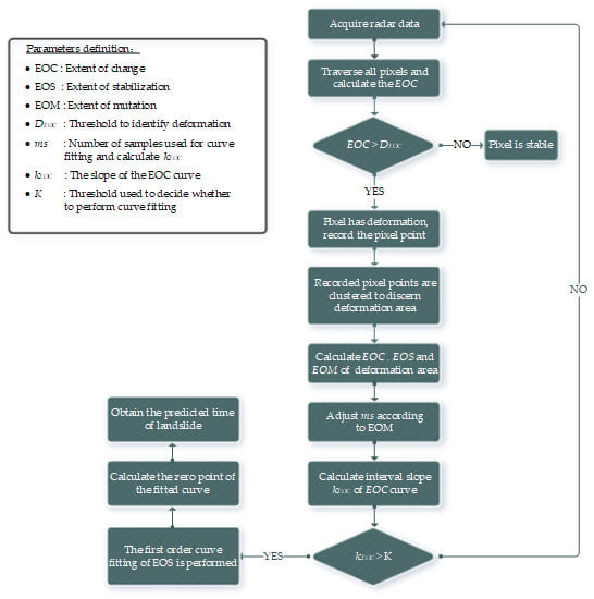
3.1. Data-Processing Flow

The data-processing flow is shown in Figure 4. As mentioned above, the ground-based micro-deformation monitoring radar can obtain large-area deformation information at one time and present it in the form of a point cloud. When obtaining radar data for a time series, all pixels of the data are first traversed, and the EOC (extent of change) is calculated. Then the point set is used as a unit to compare the EOC of each point set with the threshold D_EOC. When the EOC of the point set is greater than D_EOC, it indicates that the corresponding position of the point set is deformed; then the point set is selected. In this way, multiple point sets can be selected, and these point sets need to be classified and selected. Neighboring point sets will be divided into the same area. Eventually, many point sets are divided into several deformation regions. Each deformation region is considered an independent monitoring target.

After determining the monitoring targets, their EOC, EOS (extent of stability), and EOM (extent of mutation) can be calculated, which are also the main parameters for predicting the landslide time. Then, the slope, k_EOC, of the EOC curve can be calculated. If k_EOC is greater than threshold K, first-order curve fitting of the EOS is performed. The landslide time can be predicted based on the current deformation trend, that is, the zero point of the fitted result, which is similar to inverse velocity. At the same time, in order to improve the ability to respond to emergencies, we must always pay attention to the EOM of the target. When the EOM increases rapidly, it means that the slope deformation is accelerated, and a landslide may occur in advance. Therefore, the number of samples, m, for curve fitting needs to be adjusted according to the magnitude of the EOM.

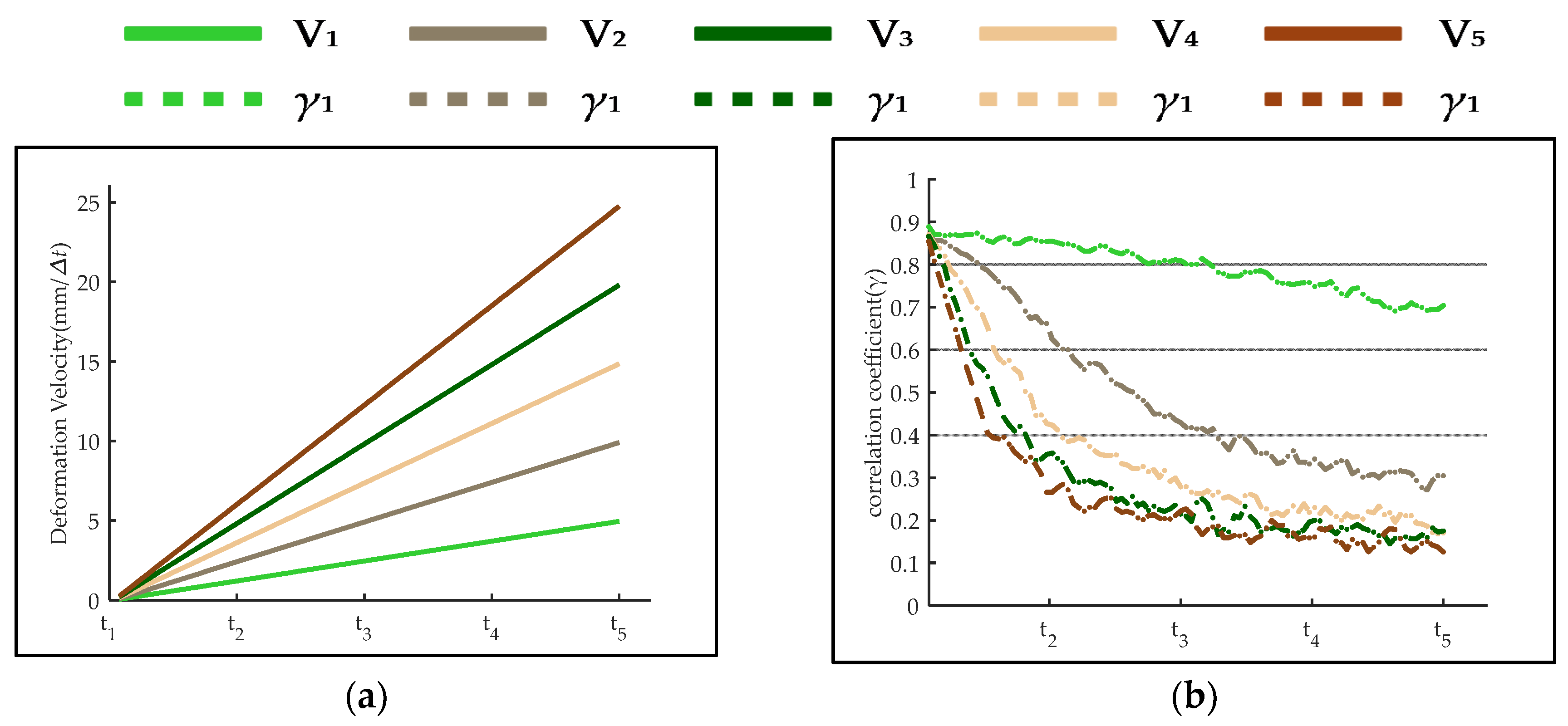
3.2. Deformation Velocity and Coherence Coefficient

The echo phase of the ground-based micro-deformation monitoring radar not only contains the distance information between the sensor and the ground target, but also includes the reflection characteristics of the ground target to the radar signal [34], as shown in Equation (1):

$$C=A\times \exp \left(\mathrm{i}\left[-\frac{4\pi }{\lambda }R+{\varphi }_{\mathrm{obj}}\right]\right)$$

(1)

where C is the radar echo, A is the backscatter coefficient of the target, 4π is the two-way distance phase, R is the slant distance between the radar and the target, λ is the wavelength, and φ_obj is the scattering phase of the target, which is determined by the target’s own properties. For the resolution unit (one pixel) of a radar image, when the target deforms, the slant distance R of the target in the unit will change, and the corresponding scattering characteristics will also change; that is, the radar echo after deformation is as follows:

$$C_1=A\times \exp \left(\mathrm{i}\left[-\frac{4\pi }{\lambda }\left(R+\Delta R\right)+{\varphi }_{\mathrm{obj}}\right]\right)\times A_1\times \exp \left(\mathrm{i}\Delta \beta \right)$$

(2)

where ΔR is the deformation value of target, and A₁•exp(iΔβ) is the radar echo change, which is caused by a change in scattering characteristics and could change the scattering phase (Δβ) and the scattering coefficient (A₁) at the same time. Therefore, Equation (2) can also be expressed as follows:

$$C_1=A\times A_1\times \exp \left(\mathrm{i}\left[-\frac{4\pi }{\lambda }\left(R+\Delta R\right)+\left({\varphi }_{\mathrm{obj}}+\Delta \beta \right)\right]\right)$$

(3)

After multiplying the first radar echo signal by the conjugate of the second echo signal and taking the phase difference, the phase change of the two echoes and the target deformation value can be obtained as follows:

$$\Delta \phi =\mathrm{phase}\left(C\times C_1^{*}\right)=-\frac{4\pi }{\lambda }\Delta R+\Delta \beta$$

(4)

$$\Delta R=-\frac{\lambda }{4\pi }\left(\Delta \phi -\Delta \beta \right)$$

(5)

where * is the complex conjugate. The change of scattering characteristics of the target will affect the result of the inversion deformation value. However, if a different scatterer is randomly distributed, the change of the scattering phase is more random, which can be suppressed by filtering [41]. On the other hand, the effect of deformation inversion is also influenced by the coherence of the target. Only when the coherence is good is it meaningful to extract the interferometric phase for deformation retrieval. In practice, the method of window estimation is often used to calculate the coherence coefficient of the same target at different moments [42]:

$$\gamma =\left|\frac{{\displaystyle \sum _{i=1}^n{C}_i\times C_{1,i}^{\ast }}}{\sqrt{{\displaystyle \sum _{i=1}^n{\left|S_i\right|}^2}\times {\displaystyle \sum _{i=1}^n{\left|S_{1,i}^{\ast }\right|}^2}}}\right|$$

(6)

where n is the number of pixels in the window, and S and S₁ are substituted into the above equation to obtain the coherence coefficient of the target as follows:

$$\gamma =\left|\frac{{\displaystyle \sum _{i=1}^n{A}_i^2{A}_{1,i}\exp \left(i\left[-\frac{4\pi }{\lambda }\Delta R+\Delta \beta \right]\right)}}{\sqrt{{\displaystyle \sum _{i=1}^n{\left|A_i\right|}^2}\times {\displaystyle \sum _{i=1}^n{\left|A_i{A}_{1,i}\right|}^2}}}\right|$$

(7)

If the target has no change in the two echoes, then ΔR and Δβ in the above equation are equal to 0, and A_1,i is equal to 1, then the coherence coefficient of the target is equal to 1, indicating that the target is completely coherent, as a value closer to 1 means that the target is more coherent. If the target moves within the time to receive the two echoes, the coherence coefficient will be between 0 and 1. When the coherence coefficient reaches 0, the target is completely irrelevant. The closer to 0, the weaker the coherence and the greater the deformation.

Theoretically, the calculations of deformation and the coherence coefficient are independent of each other, but at the same time, good coherence is a prerequisite to extracting deformation values. The area studied in this paper was formed by the accumulation of rocks, gravels, and soil after the collapse of the mountain in 2014, and this type of terrain is a relatively unconsolidated structure. Due to the motion of the target, the geometry of the target may be changed, thereby changing the scattering characteristics [43]. Therefore, the surface motion of each scattering center in each resolution unit can cause a change in coherence, which is also called the temporal decorrelation [44]. The time interval between the two images is called the time baseline; generally, there is a nonlinear inverse relationship between the time baseline and the coherence. Zebker and Villasenors performed simulations based on SeaSat parameters in one of their studies. It was concluded that, when the time baseline, wavelength, and incidence angle are constant, there is also a nonlinear inverse relationship between deformation velocity and coherence [43,44].

This paper validates the above conclusions through a simplified simulation. As shown in Figure 5, it is assumed that there is a line target within the radar monitoring range, and the line target is composed of multiple point targets. In order to simulate the change of the surface scattering characteristics caused by motion, a set of random phases satisfying the Gaussian distribution is introduced into the radar echo of the targets after each motion [45]. The standard deviation of the Gaussian distribution function is proportional to the deformation velocity, which is σ = Q * v [46]. Q is the influence factor, which indicates the degree to which the surface scattering characteristics are affected by motion, and it is set as Q = 1 here. Meanwhile, in order to simplify the simulation, the expectation value of the Gaussian distribution function is also 1. The signal released by the radar in the simulation is the frequency modulated continuous wave (FMCW), and some parameters are shown in

Table 2. Radar simulation parameters.

Frequency	Bandwidth	Simulation Range
Ku	500 MHz	10 m to 3 km

. The preset deformation velocity is shown in Figure 6a, and the coherence changes under different deformation velocity are shown in Figure 6b.

In Figure 6a, t₁–t₅ represent the simulation time. The simulation presets five groups of deformation velocity, all of which increase linearly with time, but the acceleration is different. Finally, the coherence change trend at different deformation rates shown in Figure 6b is obtained. It can be seen that if the surface motion affects the surface scattering characteristics, there is indeed a nonlinear inverse relationship between deformation velocity and the coherence. In addition, when the impact factor Q in the simulation is a constant value, the faster the deformation velocity increases, the faster the coherence decreases.

3.3. EOC, EOS, and EOM

According to the previous section, variation of the deformation trend can indirectly affect the variation of the target coherence coefficient, and the deformation velocity of the target is inversely proportional to the coherence coefficient. EOC, used to describe the extent of change of the target in per unit of time, is introduced and proposed in this paper. Compared with the deformation velocity, the EOC introduces the change of target coherence in the calculation, expressed as:

$$EOC={\displaystyle \sum _{t=T-\Delta w}^T\left(D_{lastest}\times p_t\right)}$$

(8)

where T is the current moment; Δw is the width of the time window, and when Δw = 0, the calculated result is the EOC of the target within a single radar monitoring period (two radar echoes); and D_lastest is the deformation value, which varies from case to case. If the coherence coefficient of time, t, is greater than the threshold, then D_lastest is the deformation value of time, t. Conversely, if the coherence coefficient of time (t) is less than the threshold, then D_lastest is the maximum deformation value of the moment earlier t, but the coherence coefficient of the moment is greater than the threshold. According to the prior information of the study area, the deformation information we obtain is relatively credible when the coherence coefficient of the monitoring target is greater than or equal to 0.7. Therefore, the coherence coefficient threshold used in this paper is 0.7. Moreover, p_t is the change coefficient between the deformation velocity and the coherence coefficient. The expression of p_t is as follows:

$$p_t=\frac{1-({\gamma }_t-{\gamma }_{lastest})}{{\gamma }_t}$$

(9)

where γ_t is the coherence coefficient of time, t; and γ_lastest is the coherence coefficient corresponding to D_lastest.

In addition, the EOC can be used to describe the variation of any target, whether it is a pixel or an area. When the target is an area, its EOC is equal to the weighted sum of the EOC of all pixel points in the area, and the weight is the proportion of the area represented by the pixel points in the overall area. The pixels in the radar image are mapped to actual terrain as an annular sector. The size of each annular sector can be determined by the range resolution, azimuth resolution, and footprint of the radar, as follows:

$$S_{single}=\frac{\alpha }{2}\left({\left[nd+R_{\min }\right]}^2-{\left[\left(n-1\right)d+R_{\min }\right]}^2\right)=\alpha n{d}^2+d{R}_{\min }$$

(10)

where α is the azimuth resolution, d is the range resolution, n is the sampling position of the corresponding pixel in the range direction, and R_min is the close range of radar detection. The size of the whole target is the sum of the areas of all the included pixels:

$$S_{total}={\displaystyle \sum _{i=1}^N{S}_{single,i}}=\alpha d^2{\displaystyle \sum _{i=1}^N{n}_i}+Nd{R}_{\min }$$

(11)

where N is the number of pixels contained in the deformation area. S_single,i is the area size of the i^th pixel point, and S_total is the area size of the whole target. According to Equations (8)–(11), EOC can be expressed as follows:

$$EOC={\displaystyle \sum _{t=T-\Delta w}^T{\displaystyle \sum _{i=1}^N\left(D_{lastest,i}\times \left[\frac{1-\left({\gamma }_{ti}-{\gamma }_{lastest,i}\right)}{{\gamma }_{ti}}\right]\times \frac{S_{single,i}}{S_{total}}\right)}}$$

(12)

where D_lastest,i is the D_lastest of the i^th pixel point, and γ_lastest,i is the coherence coefficient corresponding to D_lastest,i.

EOS is used to describe the extent of stability in per unit of time. EOS and EOC are reciprocal to each other in expression. If the corresponding target and time window width of both are the same, then they are also the reciprocal to each other in value:

$$EOS=EO{C}^{-1}={\displaystyle \sum _{t=T-\Delta w}^T{\displaystyle \sum _{i=1}^N\left({\left[D_{lastest,i}\times p_{ti}\right]}^{-1}\times \frac{S_{total}}{S_{single,i}}\right)}}$$

(13)

In contrast, EOM describes the extent of mutation of the target, which represents mutation of the target in one data acquisition cycle, and is given by the following equation:

$$EOM={\displaystyle \sum _{t=T-T_C}^T{\displaystyle \sum _{i=1}^N\left(D_{lastest,i}\times p_{ti}\times \frac{S_{single,i}}{S_{total}}\right)}}$$

(14)

where T_C is the radar data acquisition cycle.

EOC, EOS, and EOM are important parameters in the landslide warning method proposed in this paper. In general, the faster the deformation trend of the target is, the larger the EOC and the smaller the EOS. When the EOS is 0, it means that a landslide is coming. The EOM can help to obtain more accurate prediction results when the deformation trend of the target changes suddenly.

3.4. Discern Deformation Area

In general, people want to clearly identify potential landslide areas in monitoring data. This can be achieved by selecting some parameters for real-time monitoring and setting monitoring thresholds, because the characteristics exhibited by potential landslide areas must be different from those that are stable, such as deformation velocity or cumulative deformation value [47,48,49,50,51]. In this method, the EOC value of the potential landslide area should be larger. Therefore, the EOC can be calculated by traversing all of the pixels in the radar image, and the threshold D_EOC can be set to identify whether the pixels are in the deformation state. As long as the calculated value is greater than the threshold, the pixel will be considered as deformed.

Due to some uncontrollable factors in the monitoring environment, such as human activity, local vibration caused by construction, and the noise of the system itself, there may be numerical fluctuations in the monitoring data. If a single pixel is taken as the discernment unit during traversal, some pixels with numerical fluctuations may be mistaken for deformable pixels. However, if an area is in a deformation state, the deformation trend should be continuous and the region should not be an isolated pixel. Thus, the set of pixel points of a certain size should be taken as the discernment unit, and the EOC of each point set should be calculated during the traversal process. If the calculated value is greater than the threshold value, the region corresponding to the point set will be considered to be undergoing deformation.

As shown in Figure 7, the size of a point set is a × b, and the EOC of the point set is determined by the following:

$$EOC={\displaystyle \sum _{t=T-\Delta w}^T{\displaystyle \sum _{i=1}^{a\times b}\left(D_{lastest,i}\times p_{ti}\times \frac{S_{single,i}}{S_{total}}\right)}}$$

(15)

where a and b should not be too small; otherwise, they will still be affected by data fluctuations, resulting in misjudgment. They also should not be too large; otherwise, the point set may contain too many stable pixels, especially in the edge region of the landslide body, so that the EOC of the point set is pulled down, resulting in missed judgment. The specific value should be determined according to the actual situation in the field, and the width Δw of the time window is also the same. The EOC under different Δw can be calculated separately, to better deal with the actual situation.

In general, many independent point sets can be obtained by this method. On this basis, the point sets should be clustered. If the two point sets are adjacent or close in distance, they should be divided into the same slide body. In the end, all of the point sets will be divided into one or several landslides bodies. For those isolated point sets, they can be regarded as interference and discarded. Specifically, the Euclidean distance, L_E, between each point set is calculated with the pixel point located at (1,1) of each point set as a reference:

$$L_E\left(P_i,P_j\right)={\left[{\left(x_i-x_j\right)}^2+{\left(y_i-y_j\right)}^2\right]}^{\frac{1}{2}}$$

(16)

Meanwhile, the distance threshold D_L is also set; if the Euclidean distance between the two points is less than D_L, they are considered to belong to the same landslide body.

If we choose different deformation thresholds (or different distance thresholds or different time window widths, or subsets with different sizes), the recognition results of the deformed regions will also be different. However, the common part of multiple discernment results should be the deformed area. On this basis, the one with the largest discernment range can be selected as the final discernment result.

3.5. Landslide Prediction

As mentioned above, the more rapidly the target deforms, the smaller the EOS is, and when the EOS equals 0, a landslide may be coming soon. However, it can be seen from Equation (13) that, unless the target pixel completely loses coherence, the EOS will not be equal to 0, and will only approach 0 infinitely. On the other hand, when the EOC curve at some stage shows a rapid trend and the trend is rapid, it can be considered that the target is starting to accelerate, and at this time, the curve fitting of the EOS must be performed, as follows:

$$K<k_{EOC}=\frac{EO{C}_T-EO{C}_{T-T_c\cdot m}}{m}$$

(17)

where K is the preset slope threshold, k_EOC is the slope of the EOC curve, and m is the number of samples used to calculate the slope, as well as the number of samples used to fit the curve. Then the fitting results can be used to predict the time when the EOS reaches zero, and this moment can be taken as the possible moment of the landslide.

The least square is adopted in the curve fitting process [52]. When using this method, the first step is to determine the form of the curve. Since the form of the deformation curve of the target is close to the first-order polynomial in a window with limited width, the form of the fitting curve is F(x) = a₀ + a₁x, and it can be solved by the system of equations Ga = d:

$$\begin{array}{l}a={\left(a_0,a_1\right)}^{{\rm T}}\\ d={\left(d_0,d_1\right)}^{{\rm T}}\\ G=\left(\begin{array}{cc}\left({\varphi }_0,{\varphi }_0\right)& \left({\varphi }_0,{\varphi }_1\right)\\ \left({\varphi }_1,{\varphi }_0\right)& \left({\varphi }_1,{\varphi }_1\right)\end{array}\right)\end{array}$$

(18)

where the matrix, G, and vector, d, can be obtained by the following equations:

$$\begin{array}{l}\left({\varphi }_j,{\varphi }_k\right)={\displaystyle \sum _{i=1}^m\omega \left(x_i\right){\varphi }_j\left(x_i\right)}{\varphi }_k\left(x_i\right),\\ \begin{array}{ccc}\left(f,{\varphi }_k\right)={\displaystyle \sum _{i=1}^m\omega \left(x_i\right)f\left(x_i\right)}{\varphi }_k\left(x_i\right)=d_k,& j=0,1& k=0,1\end{array}\end{array}$$

(19)

Because the form of the fitting curve is a first-order polynomial, φ₀(x) = 1 and φ₁(x) = x. Moreover, ω(x) is a weight function, which represents the proportion of data at different time points in the fitting process. This study does not discuss the weight function, so ω(x) is 1. Finally, by calculating the zero point of the fitted curve, the moment at which a landslide might occur can be obtained:

$$t_{slipe}=\left(x-xn\right)\times T_C+T$$

(20)

where t_slipe is the predicted time of landslide occurrence, x is the zero point of the fitted curve F(x), xn is the sample number corresponding to the current moment, and T is the time corresponding to the current moment.

In this process, there are two parameters that need special attention: the slope k_EOC of the EOC curve and the number of samples m used in curve fitting. The slope determines whether curve fitting can be performed. As the landslide approaches, the EOC will inevitably show a rising and faster trend, so the prediction result will be more accurate if the slope is greater than or equal to threshold K. The value m needs to be adjusted according to the EOM. The adjusted expression is as follows:

$$m=m\mathrm{s}-\left|\lfloor EO{M}_T\times \frac{EO{M}_T}{\mathrm{E}\left(EOM\right)}\rfloor \right|$$

(21)

where ms is the initialized number of samples used in the curve fitting process; E(EOM) is the mean value of the EOM, which corresponds to the samples; the symbol $\lfloor \ast \rfloor$ means round down; and the symbol $\left|*\right|$ means take the absolute value. If the EOM increases significantly, the curve fitting needs to be implemented by appropriately shrinking m according to the mutation value, but the initialized value ms can always be adopted if the EOM trend is steady. The selection of K and m should be combined with the actual situation of the monitoring project, and will also need some human intervention. The prior information of the slope manager could be very useful at the beginning of monitoring.

4. Results

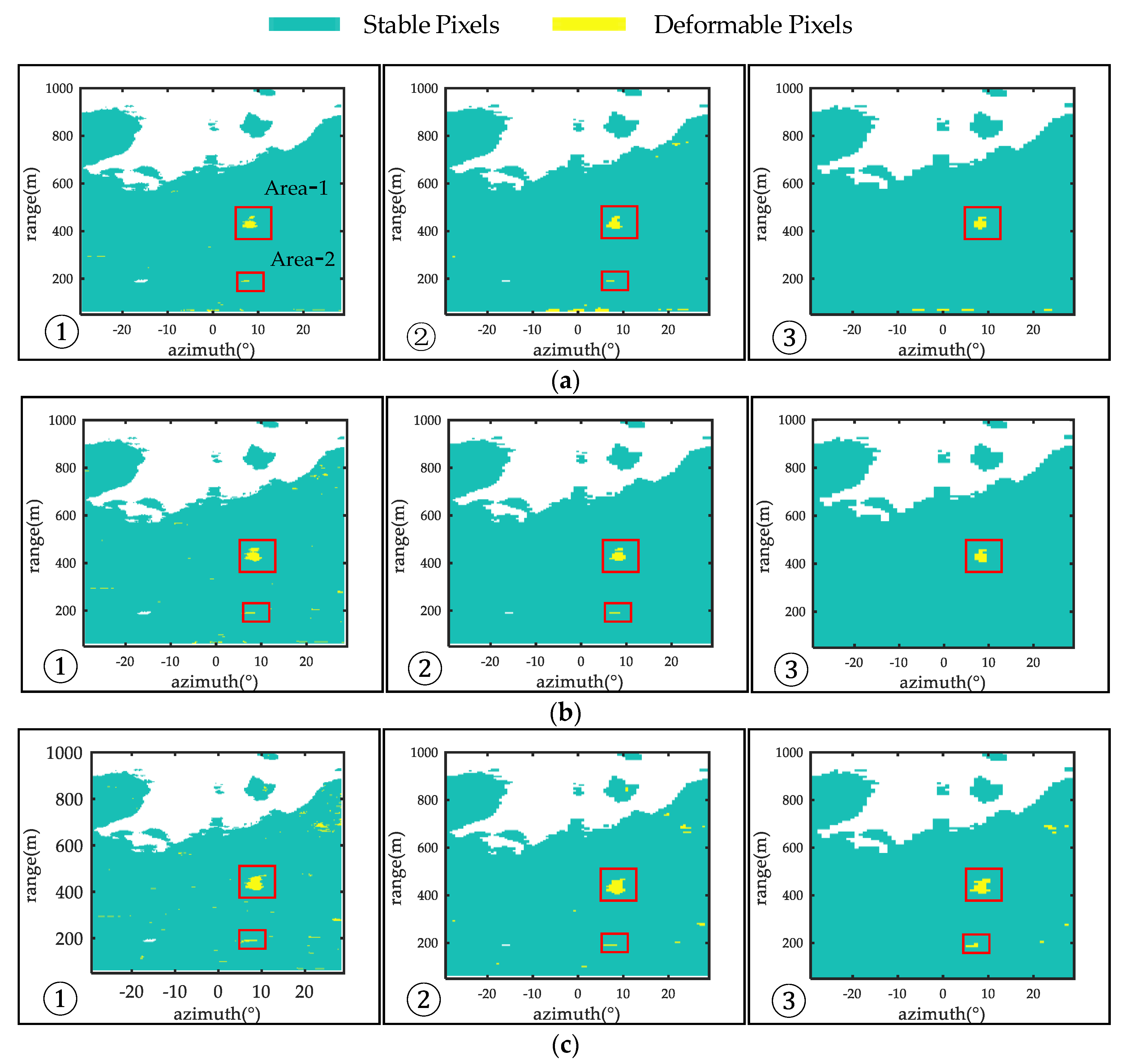
4.1. Area Discernment Result

In this paper, deformation area discernment was carried out under different parameter values. Three kinds of time windows with different widths and three kinds of point sets with different sizes were used in the discernment process, where Δw was 4, 8, and 12 h, and a × b was 10 × 1, 20 × 2, and 30 × 3. However, threshold D_EOC was always 2mm/Δw, and if the Euclidean distance between the two subsets was less than or equal to 10 m, they were considered to be merged, that is, the threshold D_L = 10. Nine discernment results were generated, as shown in Figure 8. Obviously, the Area-1 was always present in the discernment result no matter how the parameters changed, and there were also a few frequently occurring areas (such as Area-2) and some discrete point sets. We randomly selected some point sets from Areas 1 and 2, as well as other discrete point sets, and then generated their EOC curves for comparison.

During the 30 h before the landslide, there was no human activity in the shotcrete area, soft layer area, steep precipice, and drilling area, while the ground construction area was in working condition (each area is marked in Figure 1). As shown in Figure 9, the EOC value of the discrete point sets changes between [+4, −4], and there are no obvious vertices or valley points. Secondly, they also do not have a continuous upward or downward trend in the EOC values like the point sets in Areas 1 and 2. Therefore, it can be considered that the EOC values of the discrete point sets exceeding the threshold were caused by data fluctuations. For the point set in Area-2, by confirming on site that Area-2 belongs to the ground construction area, and there was human activity there from 10 to 50 h before the landslide, the working and non-working times are consistent with the characteristics shown by the curve. Therefore, it could be determined that the unevenness of the intensity of human activities caused the data to rise and fall, and then form vertices. By analogy, comparing different recognition results, only Area-1 has both a continuous deformation trend and a coherent area, and it is not in the scope of human influence. Thus, Area-1 is most likely to be a potential deformation area, which is also consistent with the actual case. The peak of the curve indicates that deformation trend of the position corresponding to the point set reaches a peak at 08:00 on the 20th, and then the deformation trend gradually decreases.

In addition, it can be seen from Figure 8 that when D_EOC and Δw are the same, increasing a × b (or decreasing Δw when D_EOC and a × b are the same) can reduce the influence of noise pixel points on the discernment results, but also lose some edge information of the deformation area. On the contrary, if more edge information is retained, more noise points will inevitably be introduced. For example, Figure 8(c1) uses a larger time window Δw and a smaller point set size a × b. It therefore captured more deformation information, but also received more interference. In contrast, there is only slight interference in Figure 8(a3,b3), but it also sacrifices much useful information. Therefore, the recognition results of this region and its surrounding pixels under different parameter values should be compared, and the one with the largest connected range should be selected as the final discernment result. According to the statistical results in

Table 3. Boundary of discernment area with different time window widths and point set sizes.

Time Window Width Δw (h)	Point Set Size (a × b)	Boundary of Deformation Area-1
		Range (m) (Near/Far)	Azimuth (°) (Left/Right)
4	10 × 1	404.2/457.2	6.7/10.0
4	20 × 2	404.2/458.1	6.7/10.0
4	30 × 3	401.1/455.1	7.3/9.7
8	10 × 1	400.2/454.5	6.1/10.6
8	20 × 2	404.2/458.1	6.7/10.0
8	30 × 3	402.4/463.2	7.0/10.6
12	10 × 1	349.5/469.2	6.1/10.6
12	20 × 2	386.4/464.4	6.4/10.6
12	30 × 3	401.1/464.4	6.4/10.6

, it was finally determined that the range of the deformation zone in radar coordinates was 349.5 to 469.2 m in range, and 6.1° to 10.6° in azimuth.

4.2. Landslide Prediction Results

Figure 10 shows the results of the data comparison between the EOC over 8 min and the velocity over 8 min of landslide area for 30 h before the landslide; 8 min is the data acquisition cycle of the on-site radar, meaning that each point on the curve corresponds to only one scene of radar data. The EOC is obtained by Equation (12).

Figure 10a shows the EOC and velocity curves. Subsequently, four representative moments, t₁ to t₄, were selected, and the velocity, 1/γ, and EOC at the four moments are shown in Figure 10b–e. The velocity used here is the deformation value obtained by processing two radar echoes. Moreover, 1/γ is the reciprocal of where the coherence between the two adjacent radar echoes. Using 1/γ can result in a large value when the coherence is reduced or even decorrelated, thereby reflecting the change of coherence more intuitively. In the time periods ts₁ and ts₂, the deformation velocity of the landslide area is not zero only at some moments, but the value of 1/γ at t₂ and t₄ is large, indicating that the loss of coherence in the landslide area during these periods may be very serious, and the prerequisite for obtaining the deformation value may be lost.

In order to verify the actual situation, the average time-series coherence of the entire landslide area was calculated. At the same time, three reference points, P₁–P₃, were selected in the landslide area, and their time-series coherence was also obtained. The results can be seen in Figure 11. Periods ts₁ and ts₂ did experience a significant decrease in coherence, either in the entire region or a single reference point. It means that the landslide area is changing rapidly, thus changing the original scattering characteristics and reducing the coherence. At the same time, the area may have experienced relatively rapid movement twice before the landslide.

The rapid movement caused a significant reduction in the coherence, making the system lose the prerequisite for obtaining the deformation value and unable to obtain effective deformation data. In contrast, as can be seen from Figure 10, if the change in coherence is added in the calculation, the deformation trend of the landslide area in the two periods can be reproduced. If the coherence is good, the EOC value will be similar to the velocity. Therefore, compared to the velocity, the EOC not only meets the needs of monitoring under normal conditions, but also provides much accurate deformation information in extreme conditions.

The above is to illustrate the effect of introducing the coherence coefficient. In actual landslide prediction, the prediction results with different Δw should be compared, to reduce the impact of data noise on the results, similar to the approach in Section 4.1. In this section, Δw values of 4, 8, and 12 h are used as examples to discuss the prediction results under different Δw.

Figure 12 shows the EOC trends and velocity trends at different Δw. This paper proposes EOC to express the extent of target change. Generally, a larger EOC means faster deformation, and smaller means a stable target. The method proposed in this paper, using EOC to reproduce the deformation trends of the two periods ts1 and ts2, improves the integrity and accuracy of the data. Therefore, the apex of the EOC curve appears earlier than the apex of the velocity curve, and the peak is larger and closer to the actual case.

Figure 13 shows the EOS trends and inverse velocity trends with different Δw. EOS and EOC are the inverse of each other, so the peak meaning of EOS should correspond to the meaning of the bottom of EOC. Thus, the larger the EOS, the more stable the target and the smaller the deformation. For example, EOS over 4 h uses a narrow time window, so it can better reflect changes in short-term data. According to the data, the study area experienced rapid movement twice before the landslide occurred, with a break of several hours between the two movements. During this period, the deformation tendency was relatively mild. Therefore, the value of EOS over 4 h in this period was increased and reaches a peak when the target was relatively stable.

The prediction results with multiple sets of parameter values are given below. In addition, since this is an inversion analysis, the actual landslide time is known (approximately at 13:50 on 20 July), so the prediction result will be presented as the difference between predicted and the actual time.

Since the changes in each stage of this case are obvious, threshold K is easy to determine, and it was set to 0.5. Two initial ms values (10 and 20) were selected as initial values of the number of samples used for curve fitting, and m was changed according to the EOM. If the EOM value increases sharply, the number of samples used for curve fitting will decrease accordingly. At the same time, m cannot be reduced infinitely, and the minimum cannot be less than 1; otherwise, curve fitting cannot be completed.

According to the above, there were two rapid changes in the target within 30 h before the landslide occurred, and the coherence was greatly reduced in these two periods, so that some deformation data were missed. By introducing a change of the coherent coefficient, the EOC has reproduced the changes in these two periods to a certain extent. Therefore, for such special cases, the use of the EOC can respond to deformation earlier and reduce the loss of effective information. It also gives more accurate and reasonable prediction results when the change trend changes suddenly or a landslide is coming. As can be seen from Figure 14 and

Table 4. Prediction error with EOS and inverse velocity at different parameters.

Δw(h)	Landslide Countdown (h)	ms = 10		ms = 20
		Prediction Error of EOS (h)	Prediction Error of Inverse Velocity (h)	Prediction Error of EOS (h)	Prediction Error of Inverse Velocity (h)
4	13	0.78	–	−2.57	−7.18
	5	–	2.03	--	1.39
	1	−0.11	–	−0.11	–
8	13	4.33	−4.21	1.16	−7.35
	5	–	0.59	–	−2.01
	1	−0.11	–	−0.11	–
12	13	2.49	3.37	−0.74	−6.92
	5	–	1.09	–	−1.95
	1	1.30	–	5.59	–

Dash (–) indicates that the data at this moment did not meet the conditions for landslide prediction. Negative error value indicates that prediction time was ahead of the landslide time; otherwise, the positive error value indicates that prediction time was behind the landslide time.

, in this case, when Δw is 4 h or 8 h, the prediction error of the result by the EOS at 1 h before the landslide is only 6.6 min. However, the prediction information cannot be obtained during this period through inverse velocity. At the same time, during the calculation of EOS (EOC) and curve fitting, the choice of the time window width Δw and initialized number of samples ms will affect the results. When Δw and ms are large, the landslide time will be predicted too late. However, if Δw and ms are small, they will be affected by data noise. Therefore, the appropriate value should be selected according to the actual situation.

The deformation process of the landslide area can be clearly seen in Figure 15. At the same time, by combining the results from the radar with digital surface model (DSM) data, we can also accurately locate where the landslide will occur. This can further improve the accuracy of landslide monitoring and will also be of great benefit to landslide prevention and treatment.

5. Discussion

In this paper, based on the time-series monitoring data of ground-based micro-deformation monitoring radars, the three parameters—extent of change (EOC), extent of stability (EOS), and extent of mutation (EOM)—are calculated according to deformation value, coherence, and deformation pixels’ size. Then a method for landslide prediction by combining these three parameters with the inverse velocity method is proposed. The method can provide earlier response actions and more accurate prediction results under extreme conditions, such as rapid deformation. The following points in the experimental processes and results are worth discussing.

As mentioned above, if surface deformation can affect the scattering characteristics of the target, then there is a nonlinear inverse relationship between deformation velocity and coherence. The main feature of the method presented in this paper is that it relies on this relationship in the process of landslide prediction, and provides a remedial measure when the coherence loss is serious, so as to obtain more accurate prediction results. Of course, it is also possible to shorten the radar revisit interval to fundamentally improve coherence, or to save some data by decreasing the coherence threshold. For this study, the revisit interval of the radar is a constant value (8 min), and the effect of decreasing the coherence threshold is not ideal. As shown in the Figure 16a, the coherence of landslide area in period ts₂ was reduced to 0.1, even lower. In this case, the information obtained by decreasing the coherence threshold is still not credible.

This paper made use of the nonlinear inverse ratio relationship between deformation velocity and coherence, and put forward the proportional coefficient p_t (Equation (9)) based on the monitoring experience. According to the description in Section 3.2, the value of γ_lastest will not be changed frequently and will not be less than the coherence threshold. Based on the research background of this paper, we set γ_lastest equal to 0.7, 0.8, and 0.9, respectively, and the relationship between γ_t and p_t is shown in the Figure 16b. As can be seen, the result conforms to the inverse proportional function and is similar to Figure 6b. Thus, it can be regarded as the proportional relationship between the deformation velocity and the coherence, which has universal applicability. However, if the object has good coherence in the deformation process, then it is difficult for the method to reflect its advantage. On the other hand, due to the differences of surface characteristics in different regions, it is difficult for the method in this paper to accurately reproduce all the data that are missing due to loss of coherence. Therefore, it is worth studying the influence of surface motion on the scattering characteristics of the ground. If this relationship can be fully understood, the proportional coefficient p_t in different environments can be targeted to obtain more accurate values. However, the radar echo is affected not only by the fine structure of the irradiated area, but also the climatic factors in the irradiated area, such as rain, snow, sand, and dust. It even varies with the incident angle of the transmitting wave, the receiving wave, and the radar frequency, so the relationship is very complicated. It needs a lot of data accumulation and analysis to realize. On the other hand, in the process of parameter selection, this paper refers to the previous observation experience and adds human intervention. How to further improve the autonomy and adaptability of systems and methods will be the focus of future work.

6. Conclusions

Landslides have become an important factor affecting modern societal and economic development, as well as individual safety [3,53]. In this study, we proposed a landslide prediction method based on a ground-based micro-deformation monitoring radar. This method combines the deformation value, coherence, and the size of the deformation area; proposes the extent of change (EOC), the extent of stability (EOS), and the extent of mutation (EOM); and uses them to predict landslides. Among them, the introduction of coherence allows the method to provide more accurate and reasonable prediction results for slope managers when the target deformation trend is too fast. On the one hand, the introduction of the size of the deformation area can clarify the deformation range, and on the other hand, it can make the deformation values of those farther pixels have a more positive impact on the results of deformation inversion of the entire area. Based on the experimental result of measured data from a landslide in Yunnan Province, China, this method achieves flexible, rapid estimation and can provide a timelier response when conditions such as excessive deformation occur.

The distribution of landslides is very wide, and the characteristics and environment are very complicated. Although it can be determined that the relationship between coherence and deformation is inversely proportional, trying to accurately confirm the proportions is still a huge challenge. The determination of other thresholds also needs to be adapted to local conditions. Although prior information can be used as an important reference, it is not enough. This requires a detailed investigation of the monitoring site. At the same time, the factors that induce landslides are diverse, so they can be a human factor or natural factors. Considering multiple factors together can further improve the efficiency of landslide prediction.

References

1. Lin, Q.; Wang, Y. Spatial and temporal analysis of a fatal landslide inventory in China from 1950 to 2016. Landslides 2018, 15, 2357–2372. [Google Scholar] [CrossRef]
2. Zhang, S.F.; Wang, Y.F.; Jia, B. Spatial-temporal changes and influencing factors of geologic disasters from 2005 to 2016 in China. J. GeoInf. Sci. 2017, 19, 1567–1574. [Google Scholar]
3. Froude, M.J.; Petley, D. Global fatal landslide occurrence from 2004 to 2016. Nat. Hazards Earth Syst. Sci. 2018, 18, 2161–2181. [Google Scholar] [CrossRef] [Green Version]
4. Wang, Y.; Zhang, N.N.; Sun, Z.; Fei, W. The major domestic natural disasters in 2017. Disaster Reduct. China 2018, 5, 38–41. [Google Scholar]
5. Liu, N.J.; Zhang, D.; Wang, Y. Inventory of major domestic natural disasters in 2018. Disaster Reduct. China 2019, 5, 18–23. [Google Scholar]
6. The Ministry of Emergency Management Announce the Ten Major Domestic Natural Disasters in 2019. Available online: https://www.mem.gov.cn/xw/bndt/202001/t20200112_343410.shtml (accessed on 12 January 2020).
7. Xu, Q.; Tang, M.G.; Huang, R.Q. Monitoring, Early Warning and Emergency Disposal of Large Landslides; Science Press: Beijing, China, 2015. [Google Scholar]
8. Zao, C.Y.; Liu, X.J. Research on landslide identification, monitoring and failure model with InSAR technique in Heifangtai, Gansu. Geomat. Inf. Sci. Wuhan Univ. 2019, 44, 996–1007. [Google Scholar]
9. Xu, Q.; Dong, X.J.; Li, W.L. Integrated space-air-ground early detection, monitoring and warning system for potential catastrophic geohazards. Geomat. Inf. Sci. Wuhan Univ. 2019, 44, 957–966. [Google Scholar]
10. Ge, D.Q.; Dai, K.R. Early identification of serious geological hazards with integrated remote sensing technologies: Thoughts and recommendations. Geomat. Inf. Sci. Wuhan Univ. 2019, 44, 949–956. [Google Scholar]
11. Atzeni, C.; Barla, M.; Pieraccini, M. Early warning monitoring of natural and engineered slopes with ground-based synthetic-aperture radar. Rock Mech. Rock Eng. 2015, 48, 235–246. [Google Scholar] [CrossRef] [Green Version]
12. Intrieri, E.; Carlà, T.; Farina, P.; Bardi, F.; Ketizmen, H.; Casagli, N. Satellite interferometry as a tool for early warning and aiding decision making in an open—Pit mine. IEEE J. Sel. Top. Appl. Earth Obs. Remote Sens. 2019, 12, 5248–5258. [Google Scholar] [CrossRef]
13. Zeng, T.; Deng, Y.K. Development state and application examples of ground-based differential interferometric radar. J. Radars 2019, 8, 154–170. [Google Scholar]
14. Carlà, T.; Intrieri, E.; Raspini, F.; Bardi, F.; Farina, P.; Ferretti, A.; Colombo, D.; Novali, F.; Casagli, N. Perspectives on the prediction of catastrophic slope failures from satellite InSAR. Sci. Rep. 2019, 9, 14137. [Google Scholar] [CrossRef] [PubMed] [Green Version]
15. Liu, P.; Li, Z.H.; Hoey, T. Using advanced InSAR time series techniques to monitor landslide movements in Badong of the Three Gorges region, China. Int. J. Appl. Earth Obs. Geoinf. 2013, 21, 253–264. [Google Scholar] [CrossRef]
16. Florentino, A.; Charapaqui, S.; De La Jara, C.; Milla, M. Implementation of a ground-based synthetic aperture radar (GB-SAR) for landslide monitoring: System description and preliminary results. In Proceedings of the IEEE XXIII International Congress on Electronics, Piura, Peru, 2–5 August 2016. [Google Scholar]
17. Shi, X.G.; Zhang, L. Detection and characterization of active slope deformations with Sentinel-1 InSAR analyses in the southwest area of Shanxi, China. Remote Sens. 2020, 12, 392. [Google Scholar] [CrossRef] [Green Version]
18. Li, W.L.; Xu, Q. Historical retrospection of deformation of large rocky landslides and its enlightenment. Geomat. Inf. Sci. Wuhan Univ. 2019, 44, 1043–1053. [Google Scholar]
19. Peng, L.; Xu, S.N.; Peng, J.H. Research on development characteristics and size of landslides in the Three Gorges area. Geoscience 2014, 28, 1077–1086. [Google Scholar]
20. Luo, W.Q.; Lu, F.A. Evolution stage division of landslide based on analysis of multivariate time series. Earth Sci. 2016, 41, 711–717. [Google Scholar]
21. Graham, J.D.; Erik, E. Development of an early-warning time-of-failure analysis methodology for open-pit mine slopes utilizing ground-based slope stability radar monitoring data. Can. Geotech. J. 2015, 52, 515–529. [Google Scholar]
22. Qin, S.Q.; Wang, Y.Y.; Ma, P. Exponential laws of critical displacement evolution for landslides and avalanches. Chin. J. Rock Mech. Eng. 2010, 29, 873–880. [Google Scholar]
23. Zao, C.Y.; Liu, X.J. Characteristics of landslide displacement-time curve by physical simulation experiment. J. Eng. Geol. 2015, 3, 401–407. [Google Scholar]
24. Chen, X.P.; Zhang, Q.Y.; Liu, D.W. Deformation statistical regression analysis model of slope and its application. Chin. J. Rock Mech. Eng. 2008, 27, 3673–3679. [Google Scholar]
25. Voight, B.A. Method for prediction of volcanic eruptions. Nature 1988, 332, 125–130. [Google Scholar] [CrossRef]
26. Fukuzono, T. A new method for predicting the failure time of a slope. In Proceedings of the Fourth International Conference and Field Workshop on Landslides, Japan Landslide Society, Tokyo, Japan, 23–31 August 1985; pp. 145–150. [Google Scholar]
27. Carlà, T.; Intrieri, E.; Di Traglia, F.; Nolesini, T.; Giovanni Gigli, G.; Casagli, N. Guidelines on the use of inverse velocity method as a tool for setting alarm thresholds and forecasting landslides and structure collapses. Landslides 2017, 14, 517–534. [Google Scholar] [CrossRef] [Green Version]
28. Xu, Q.; Li, W.L.; Dong, X.J. The Xinmocun landslide on 24 June 2017 in Maoxian, Sichuan: Characteristics and failure mechanism. Chin. J. Rock Mech. Eng. 2017, 36, 2612–2628. [Google Scholar]
29. Pieraccini, M.; Miccinesi, L. Ground-Based Radar Interferometry: A Bibliographic Review. Remote Sens. 2019, 11, 1029. [Google Scholar] [CrossRef] [Green Version]
30. Bardi, F.; Raspini, F.; Frodella, W.; Lombardi, L.; Nocentini, M.; Gigli, G.; Morelli, S.; Corsini, A.; Casagli, N. Monitoring the rapid-moving reactivation of earth flows by means of GB-InSAR: The April 2013 Capriglio landslide (northern Appennines, Italy). Remote Sens. 2017, 9, 165. [Google Scholar] [CrossRef] [Green Version]
31. Tarchi, D.; Casagli, N.; Fanti, R. Landslide monitoring by using ground-based SAR interferometry: An example of application to the Tessina landslide in Italy. Eng. Geol. 2003, 68, 15–30. [Google Scholar] [CrossRef]
32. Macedo, K.A.; Ramos, F.L.; Gaboardi, C. A compact ground-based interferometric radar for landslide monitoring: The Xerém experiment. IEEE J. Sel. Top. Appl. Earth Obs. Remote Sens. 2017, 99, 1–12. [Google Scholar] [CrossRef]
33. Traglia, F.; Intrieri, E.; Nolesini, T.; Bardi, F.; Del Ventisette, C.; Ferrigno, F.; Frangioni, S.; Frodella, W.; Gigli, G.; Lotti, A.; et al. The ground-based InSAR monitoring system at Stromboli volcano: Linking changes in displacement rate and intensity of persistent volcanic activity. Bull. Volcanol. 2014, 76, 1–18. [Google Scholar] [CrossRef]
34. Zhang, H.; Wang, C. Research on DInSAR Method Based on Coherent Target; Science Press: Beijing, China, 2009; pp. 12–28. [Google Scholar]
35. Tofani, V.; Raspini, F.; Catani, F.; Casagli, N. Persistent scatterer interferometry (PSI) technique for landslide characterization and monitoring. Remote Sens. 2013, 5, 1045–1065. [Google Scholar] [CrossRef] [Green Version]
36. Tian, X.; Liao, M.S. The analysis of conditions for InSAR in the field of deformation monitoring. Chin. J. Geophys. 2013, 56, 812–823. [Google Scholar]
37. Huang, Z.S.; Sun, J.P.; Li, Q.; Tan, W.X. Time- and space-varying atmospheric phase correction in discontinuous ground-based synthetic aperture radar deformation monitoring. Sensors 2018, 18, 3883. [Google Scholar] [CrossRef] [PubMed] [Green Version]
38. Zheng, X.; Yang, X.; Ma, H.; Ren, G.; Zhang, K.; Yang, F.; Li, C. Integrated Ground-Based SAR Interferometry, Terrestrial Laser Scanner, and Corner Reflector Deformation Experiments. Sensors 2018, 18, 4401. [Google Scholar] [CrossRef] [PubMed] [Green Version]
39. Ma, J.H.; Sun, J.Q.; Wang, J. Real-time prediction for 2018 JJA extreme precipitation and landslides. Trans. Atmos. Sci. 2019, 42, 93–99. [Google Scholar]
40. Luo, Y.; He, S.M.; He, J.C. Effect of rainfall patterns on stability of shallow landslide. Earth Sci. 2014, 39, 1357–1363. [Google Scholar]
41. Oliver, C.; Shaun, Q.G. Understanding Synthetic Aperture Radar Images; Artech House: Boston, MA, USA, 1998; pp. 75–119. [Google Scholar]
42. Touzi, R.; Lopes, A. Coherence estimation for SAR imagery. IEEE Trans. Geosci. Remote Sens. 1999, 37, 135–149. [Google Scholar] [CrossRef] [Green Version]
43. Guo, L.P.; Yue, J.P. Analysis coherence effected by baseline and time interval. Bull. Surv. Mapp. 2018, 7, 9–12. [Google Scholar]
44. Zebker, H.A.; Villasenor, J. Decorrelation in interferometric radar echoes. IEEE Trans. Geosci. Remote Sens. 1992, 30, 950–959. [Google Scholar] [CrossRef] [Green Version]
45. Kuga, Y.; Phu, P. Experimental research of millimeter wave scattering in discrete random media and from rough surfaces. Prog. Electromagn. Res. 1996, 14, 37–88. [Google Scholar]
46. Wang, Y.H.; Yu, Y.; Zang, Y.M. Investigation on synthetic aperture radar imaging simulation of oceanic wind waves. Trans. Oceanol. Limnol. 2019, 6, 41–47. [Google Scholar]
47. Guo, R.; Li, S.M.; Chen, Y.N. A method based on SBAS-InSAR for comprehensive identification of potential goaf landslide. J. GeoInf. Sci. 2019, 21, 1109–1120. [Google Scholar]
48. Tripolitsiotis, A.; Steiakakis, C.; Papadaki, E. Complementing geotechnical slope stability and land movement analysis using satellite DInSAR. Cent. Eur. J. Geosci. 2014, 6, 56–66. [Google Scholar] [CrossRef] [Green Version]
49. Zhang, L.; Liao, M.S.; Dong, J. Early detection of landslide hazards in mountainous areas of west China using time series SAR Interferometry-a case study of Danba, Sichuan. Geomat. Inf. Sci. Wuhan Univ. 2018, 43, 2039–2049. [Google Scholar]
50. Jaedicke, C.; Eeckhaut, M.V.; Nadim, F. Identification of landslide hazard and risk ‘hotspots’ in Europe. Bull. Eng. Geol. Environ. 2014, 73, 325–339. [Google Scholar] [CrossRef] [Green Version]
51. Sun, J.L.; Ma, J.H.; Dong, G.F. Analysis of surface deformation characteristics and identification of potential landslides in Gaojiawan area. Geomat. Spat. Inf. Technol. 2019, 42, 99–103. [Google Scholar]
52. Li, Q.Y.; Wang, N.C. Numerical Analysis; Tsinghua University Press: Beijing, China, 2008; pp. 73–78. [Google Scholar]
53. Li, Z.H.; Song, C.; Yu, C. Application of satellite radar remote sensing to landslide detection and monitoring: Challenges and solutions. Geomat. Inf. Sci. Wuhan Univ. 2019, 44, 967–979. [Google Scholar]
Figure 1. Schematic diagram of area division. The coordinate system in diagram is a local coordinate system for terrain sampling, and coordinate unit is m.
Remotesensing 12 01230 g001
Figure 2. Schematic diagram of monitoring system.
Remotesensing 12 01230 g002
Figure 3. Comparison of radar image and a drone image.
Remotesensing 12 01230 g003
Figure 4. Flowchart of landslide-prediction method.
Remotesensing 12 01230 g004
Figure 5. Schematic diagram of simulation targets.
Remotesensing 12 01230 g005
Figure 6. (a) Simulation deformation velocity of the targets; (b) variation trend of the simulation targets coherence coefficient with deformation velocity.
Remotesensing 12 01230 g006
Figure 7. Schematic diagram of deformation area discernment.
Remotesensing 12 01230 g007
Figure 8. (a) Discernment results when Δw = 4 h and a × b is 10 × 1, 20 × 2, and 30 × 3; (b) discernment results when Δw = 8 h and a × b is 10 × 1, 20 × 2, and 30 × 3; (c) discernment results when Δw = 12 h and a × b is 10 × 1, 20 × 2, and 30 × 3.
Remotesensing 12 01230 g008
Figure 9. Extent of change (EOC) curves of different point sets at where Δw = 4 h and a × b is 10 × 1.
Remotesensing 12 01230 g009
Figure 10. (a) Velocity and EOC curves in the 30 h before the landslide; (b) velocity, 1/γ, and EOC at moment t1; (c) velocity, 1/γ, and EOC at moment t2; (d) velocity, 1/γ, and EOC at moment t3; (e) velocity, 1/γ, and EOC at moment t4.
Remotesensing 12 01230 g010aRemotesensing 12 01230 g010b
Figure 11. (a) Reference points location diagram; (b) time-series region average coherence of the landslide area and time-series coherence of the reference points.
Remotesensing 12 01230 g011
Figure 12. EOC and velocity trends over 4, 8, and 12 h.
Remotesensing 12 01230 g012
Figure 13. Extent of stability (EOS) and inverse velocity trends over 4, 8, and 12 h.
Remotesensing 12 01230 g013
Figure 14. Prediction errors of EOS and inverse velocity when (a) Δw = 4 h and ms is 10 and 20; (b) Δw = 8 h and ms is 10 and 20; and (c) Δw = 12 h and ms is 10 and 20.
Remotesensing 12 01230 g014aRemotesensing 12 01230 g014b
Figure 15. The fusion result of accumulated EOC data and terrain data.
Remotesensing 12 01230 g015
Figure 16. (a) Coherence map of landslide area in period ts2, Δt = 8 min; (b) the ptt curves at different γlastest.
Remotesensing 12 01230 g016