Global and Regional High-Resolution VTEC Modelling Using a Two-Step B-Spline Approach

Abstract

The ionosphere is one of the largest error sources in GNSS (Global Navigation Satellite Systems) applications and can cause up to several meters of error in positioning. Especially for single-frequency users, who cannot correct the ionospheric delay, the information about the state of the ionosphere is mandatory. Dual- and multi-frequency GNSS users, on the other hand, can correct the ionospheric effect on their observations by linear combination. However, real-time applications such as autonomous driving or precision farming, require external high accuracy corrections for fast convergence. Mostly, this external information is given in terms of grids or coefficients of the vertical total electron content (VTEC). Globally distributed GNSS stations of different networks, such as the network of the International GNSS Services (IGS), provide a large number of multi-frequency observations which can be used to determine the state of the ionosphere. These data are used to generate Global Ionosphere Maps (GIM). Due to the inhomogeneous global distribution of GNSS real-time stations and especially due to the large data gaps over oceanic areas, the global VTEC models are usually limited in their spatial and spectral resolution. Most of the GIMs are mathematically based on globally defined radial basis functions, i.e., spherical harmonics (SH), with a maximum degree of 15 and provided with a spatial resolution of ${2.5}^{°}\times 5^{°}$ in latitude and longitude, respectively. Regional GNSS networks, however, offer dense clusters of observations, which can be used to generate regional VTEC solutions with a higher spectral resolution. In this study, we introduce a two-step model (TSM) comprising a global model as the first step and a regional model as the second step. We apply polynomial and trigonometric B-spline functions to represent the global VTEC. Polynomial B-splines are used for modelling the finer structures of VTEC within selected regions, i.e., the densification areas. The TSM provides both, a global and a regional VTEC map at the same time. In order to study the performance, we apply the developed approach to hourly data of the global IGS network as well as the EUREF network of the European region for St. Patrick storm in March 2015. For the assessment of the generated maps, we use the dSTEC analysis and compare both maps with different global and regional products from the IGS Ionosphere Associated Analysis Centers, e.g., the global product from CODE (Berne, Switzerland) and from UPC (Barcelona, Spain), as well as the regional maps from ROB (Brussels, Belgium). The assessment shows a significant improvement of the regional VTEC representation in the form of the generated TSM maps. Among all other products used for comparison, the developed regional one is of the highest accuracy within the selected time span. Since the numerical tests are performed using hourly data with a latency of one to two hours, the presented procedure is seen as an intermediate step for the generation of high precision regional real-time corrections for modern applications.

1. Introduction

In the last decades, the use of GNSS for a broad range of commercial and scientific fields has significantly increased. Especially GNSS applications which rely on high precision positioning and navigation became more and more popular. With higher demands on accuracy, the requirements for detecting and correcting errors in the measurements increase. The main error sources in precise GNSS are the effects caused by the atmosphere. Whilst the tropospheric effects can yield approximately 1m error in positioning (in along range, i.e., the height), the ionosphere effects can vary between 1 m and even 100 m. The ionosphere is defined as the part of the upper atmosphere where the number of charged particles (electrons and ions) is high enough to induce significant changes in the propagation of radio waves. The effect mainly depends on the signal frequency; signals with frequencies lower then 30 MHz can be blocked and reflected, signals with a shorter wavelength, however, are affected in their travel times (delay) and their signal paths (bending). The delay of the signal between the satellite S and the receiver R defined as

$$d_{ion}=\pm \frac{40.3}{f^2}{\int }_S^R{N}_{e}ds$$

(1)

is only an approximation as higher-order effects are neglected. The sign on the right-hand side changes whether it is applied for carrier phase observations (‘-’) or for pseudorange measurements (‘+’) [1]. In geodesy the delay can be interpreted in two ways, namely as a

• disturbing quantity which has to be corrected for precise applications or as a
• target quantity.

In the latter case, $d_{ion}$ can be used as observation to determine the electron density $N_e$ as the ionospheric key parameter. Among many others, e.g., ionosondes and radio occultations, GNSS is the most prominent observation technique used to gain information about $N_e$. However, GNSS is not sensitive to the electron density directly, but on the integrated effect along the ray path. It is denoted as Slant Total Electron Content (STEC) and defined as

$$STEC({\mathit{x}}^S,{\mathit{x}}_R,t)={\int }_S^R{N}_e(\mathit{x},t)ds.$$

(2)

STEC depends on the electron density $N_e(\mathit{x},t)$ along the ray path between the position ${\mathit{x}}^S$ of the satellite S and the position ${\mathit{x}}_R$ of the receiver R for time t. The position vector $\mathit{x}$ reads

$$\mathit{x}=r{\left[cos\phi cos\lambda ,cos\phi sin\lambda ,sin\phi \right]}^T,$$

(3)

where $\phi$ and $\lambda$ are latitude and longitude, r is the radial distance within a geocentric coordinate system ${\mathsf{\Sigma }}_E$.Many ionosphere models rely on the assumption that all electrons in the ionosphere are concentrated on a spherical shell ${\mathsf{\Omega }}_H$ of infinitesimal thickness with fixed height $H=r-R_e$ above the spherical Earth of radius $R_e$. It is denoted as single-layer model (SLM) and allows for the transformation of STEC into the vertical direction as

$$VTEC({\mathit{x}}_{IPP},t)=\frac{STEC({\mathit{x}}^S,{\mathit{x}}_R,t)}{M\left(z\right)}$$

(4)

by applying a mapping function $M\left(z\right)$ depending on the zenith angle z [2]. It yields vertical total electron content (VTEC) referred to the Ionospheric Pierce Point (IPP), the intersection point of the ray-path with the shell ${\mathsf{\Omega }}_H$ at the position ${\mathit{x}}_{IPP}$. Several approaches exist for the realization of the mapping function; recently UPC developed the Barcelona Ionospheric Mapping Function (BIMF) [3]. Besides the electron density VTEC means another ionospheric key parameter which can be represented as the integration,

$$VTEC(\phi ,\lambda ,t)={\int }_{h_l}^{h_u}{N}_e(\phi ,\lambda ,h,t)dh,$$

(5)

of the electron density along the height between the lower boundary $h_l$ and the upper boundary $h_u$ of the ionosphere.

There are several approaches for representing VTEC globally by using input data from GNSS. The Ionospheric Associated Analysis Centers (IAAC) of the International GNSS Service (IGS), namely (1) the Jet Propulsion Laboratory (JPL), (2) the Center for Orbit Determination in Europe (CODE), (3) the European Space Operations Center of the European Space Agency (ESOC), (4) the Universitat Politècnica de Catalunya (UPC), (5) the Canadian Geodetic Survey of Natural Resources Canada (NRCan), (6) the Wuhan University (WHU) and (7) the Chinese Academy of Sciences (CAS) routinely provide Global Ionosphere Maps (GIM) representing VTEC based on different mathematical approaches, namely the series expansion or the discretization technique. Whereas in the latter case, usually pixels or voxels are chosen [4], in the case of a series expansion spherical harmonics (SH) are mostly used. The GIM products of the IAACs are also used to generate an IGS GIM as a combined solution [5].

As a matter of fact, the representation of VTEC on a global scale suffers from the inhomogeneous distribution of the input data which does not allow a high-resolution representation on a global scale [6]. Capturing this inhomogeneity, the maximum degree of SHs is generally set to $n=15$. The GIMs are usually provided in IONosphere Map EXchange (IONEX) format with a temporal resolution of 2 h and a spatial sampling of ${2.5}^{°}\times 5^{°}$ with respect to latitude and longitude and with a latency of more than one week [7,8].

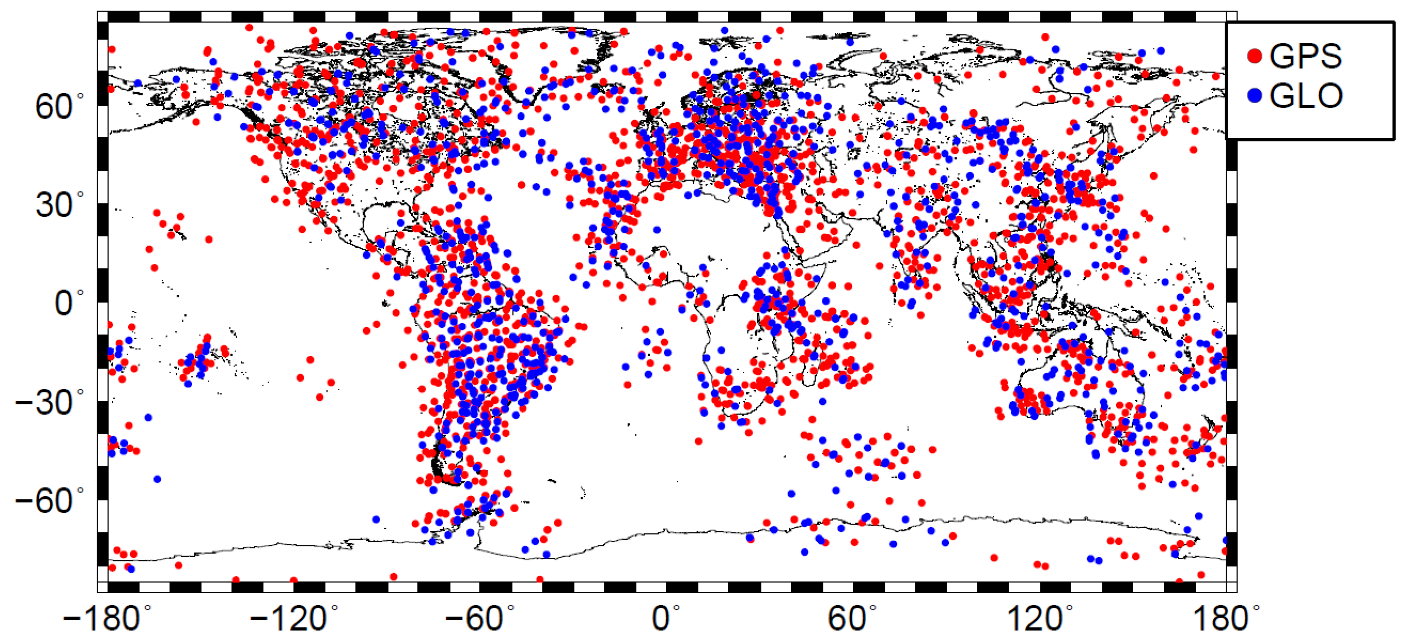
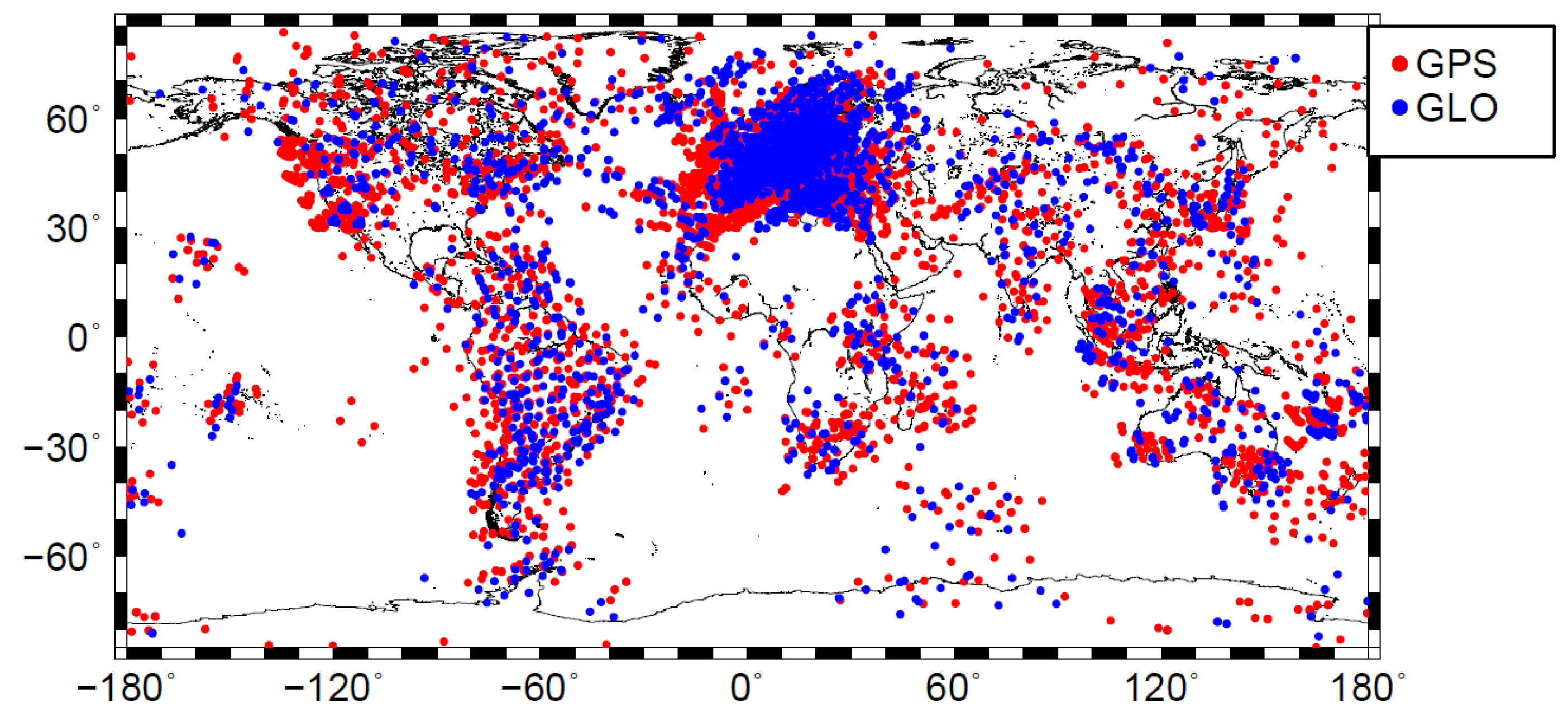
Goss et al. [9] developed an approach based on B-spline basis functions and a Multi-Scale Representation (MSR) which allows to model VTEC globally with a higher spectral resolution. B-splines have already proven to be suitable basis function for representing global VTEC [10,11,12]. However, as a matter of fact, finer ionospheric structures can only be monitored and modeled where high-resolution input data are available, i.e., in continental regions such as Europe and North America, where a large number of stations of the global network of the IGS are located. Some of the continental regions are also covered with additional stations from regional networks, e.g., EUREF for Europe, AFREF for South Africa, ARGN and SPRGN for the Australian and Pacific region. Figure 1 shows all IPPs collected at 12:00 UT from the receiver stations of IGS and EUREF. Due to the coverage of observation stations over Europe, a dense cluster of observations is available.

The Royal Observatory of Belgium (ROB) [13], for instance, provides Regional Ionospheric Maps (RIM) for the European region. Besides this, there are several approaches for the regional representation of VTEC, e.g., regional B-spline expansions [10,14,15,16], the thin plate spline (TPS) interpolation [17], the Taylor series [18] and the SH expansion using a spherical cap coordinate system [19].

In this paper, we describe a procedure to represent VTEC for regions with dense data coverage with high spatial and spectral resolution based on a two-step strategy using B-spline basis functions. In the first step, we apply a global B-spline model with polynomial B-splines for latitude and trigonometric B-splines for longitude in order to represent the long-period VTEC part globally. In the second step, we perform a densification into regions with dense data coverage by using the global model as background and estimating B-spline coefficients of tensor products of polynomial B-splines representing the finer structures of VTEC. In combination, the model allows for a high-resolution VTEC representation within the densification regions. The developed approach is denoted as two-step model (TSM).

The paper is outlined as follows: in Section 2 a general description of the modelling of VTEC is given. Additionally in Section 2.1, the two-step model, based on B-spline basis functions and the connection between the two modelling steps is derived. Section 2.2 comprises a detailed description of the estimation of the unknown model parameters using a Kalman filter. Furthermore, in Section 2.3 the products of the TSM are defined. In Section 3 the TSM is applied to the European region during the St. Patrick storm days in March 2015 with a detailed validation in Section 4.

2. Modelling Strategies for the Regional VTEC Representation

A 3-D function $VTEC(\phi ,\lambda ,t)=f(\mathit{x},t)$, as introduced in Equation (5), can be represented by means of a series expansion as

$$f(\mathit{x},t)={\displaystyle \sum _{k=0}^{\infty }}{c}_k\left(t\right){\varphi }_k\left(\mathit{x}\right),$$

(6)

wherein ${\varphi }_k\left(\mathit{x}\right)$ are given space-dependent basis functions and $c_k\left(t\right)$ are the corresponding time-dependent series coefficients. Assuming that $I_s$ observations $y({\mathit{x}}_{i_s},t_s)$ of VTEC are given at IPP positions $P_{i_s}\in {\mathsf{\Omega }}_H$ with $i_s=1,2,\dots ,I_s$ and discrete time moments $t_s=t_0+s·\mathsf{\Delta }t$ with $s\in {\mathbb{N}}_0$ and $\mathsf{\Delta }t$ being a given temporal sampling interval, the observation equation can be written as

$$y({\mathit{x}}_{i_s},t_s)+e({\mathit{x}}_{i_s},t_s)=f_N({\mathit{x}}_{i_s},t_s)={\displaystyle \sum _{k=0}^N}{c}_k\left(t_s\right){\varphi }_k\left(x_{i_s}\right),$$

(7)

with $e({\mathit{x}}_{i_s},t_s)$ being the measurement errors of the observations. Note, in the sequel of this paper, if not stated otherwise, we omit additional unknown parameters such as the satellite and receiver biases, i.e., Differential Code Biases (DCB) for the geometry free observations as on the right-hand side of Equation (7).

2.1. Two-Step B-Spline Expansion

At DGFI-TUM we rely on a two-step VTEC model (TSM) in terms of B-splines. The basic equation

$$VTE{C}_{\mathrm{reg}}(\phi ,\lambda ,t)=VTE{C}_{\mathrm{glob}}(\phi ,\lambda ,t)+\mathsf{\Delta }VTE{C}_{\mathrm{reg}}(\phi ,\lambda ,t)$$

(8)

yields VTEC within the region of interest as the sum of the global model part $VTE{C}_{\mathrm{glob}}$(first step) and the regional model part $\mathsf{\Delta }VTE{C}_{\mathrm{reg}}$ (second step).

2.1.1. Global B-Spline Model

For global VTEC modelling we rewrite Equation (7) as

$$y({\mathit{x}}_{i_s},t_s)+e({\mathit{x}}_{i_s},t_s)=VTE{C}_{\mathrm{glob}}({\mathit{x}}_{i_s},t_s)={\displaystyle \sum _{k_1=0}^{K_{J_1}-1}\sum _{k_2=0}^{K_{J_2}-1}}{d}_{k_1,k_2}^{J_1,J_2}\left(t_s\right){\varphi }_{k_1,J_1}\left({\phi }_{i_s}\right){\tilde{\varphi }}_{k_2,J_2}\left({\lambda }_{i_s}\right),$$

(9)

with $K_{J_1}·K_{J_2}$ initially unknown time-dependent series coefficients $d_{k_1,k_2}^{J_1,J_2}\left(t_s\right)$ and the tensor products

$${\varphi }_{k_1,J_1}\left({\phi }_{i_s}\right){\tilde{\varphi }}_{k_2,J_2}\left({\lambda }_{i_s}\right)$$

of polynomial B-spline functions ${\varphi }_{k_1,J_1}\left(\phi \right)$ and trigonometric B-spline functions ${\tilde{\varphi }}_{k_2,J_2}\left(\lambda \right)$ representing VTEC w.r.t. latitude $\phi$ and longitude $\lambda$; for more information see [9,20,21,22,23]. The shift parameters $k_1\in \{0,1,\dots ,K_{J_1}-1\}$ and $k_2\in \{0,1,\dots ,K_{J_2}-1\}$ for polynomial and trigonometric B-splines, define the position of the B-spline functions on the sphere ${\mathsf{\Omega }}_H$. The total numbers $K_{J_1}=2^{J_1}+2$ and $K_{J_2}=3·2^{J_2}$ of B-spline functions depend on the B-spline levels $J_1$ and $J_2$. In order to select appropriate numerical values for $J_1$ and $J_2$, the two inequality chains

$$\begin{array}{cc}\hfill J_1& \le {log}_2\left(\frac{{180}^{°}}{\mathsf{\Delta }\phi }-1\right)\le {log}_2\left(n_{max}-1\right)\mathrm{and}\hfill \\ \hfill J_2& \le {log}_2\left(\frac{{120}^{°}}{\mathsf{\Delta }\lambda }\right)\le {log}_2\left(\frac{2·n_{max}}{3}\right),\hfill \end{array}$$

(10)

have been considered by Goss et al. [9] and relate $J_1$ and $J_2$ to the average global sampling intervals $\mathsf{\Delta }\phi$ and $\mathsf{\Delta }\lambda$ of the input data, i.e., the GNSS measurements, and the maximum degree $n_{max}$ of a SH expansion, which means the measure for the spectral content of a signal given on a sphere.

For the numerical values 1 to 6 for the B-spline levels $J_1$ and $J_2$,

Table 1. Values for the B-spline levels $J_1$ and $J_2$, the maximum spherical harmonics (SH) degree $n_{max}$, the input data sampling intervals $\mathsf{\Delta }\phi$ and $\mathsf{\Delta }\lambda$, as well as the minimum wavelengths $L_{\phi }$ and $L_{\lambda }$; the left part presents the values along the meridian (upper inequalities in Equation (10)), the right part the corresponding values along the equator and its parallels (lower inequalities in Equation (10)).

	Latitude							Longitude
$J_1$	1	2	3	4	5	6	$J_2$	1	2	3	4	5	6
$n_{max}$	3	5	9	17	33	63	$n_{max}$	3	6	12	24	48	96
$\mathsf{\Delta }\phi$	${60}^{°}$	${36}^{°}$	${20}^{°}$	${10.5}^{°}$	${5.45}^{°}$	${2.85}^{°}$	$\mathsf{\Delta }\lambda$	${60}^{°}$	${30}^{°}$	${15}^{°}$	${7.5}^{°}$	${3.75}^{°}$	${1.875}^{°}$
$L_{\phi }$	${120}^{°}$	${72}^{°}$	${40}^{°}$	${21}^{°}$	${10.9}^{°}$	${5.7}^{°}$	$L_{\lambda }$	${120}^{°}$	${60}^{°}$	${30}^{°}$	${15}^{°}$	${7.5}^{°}$	${3.75}^{°}$

presents the corresponding largest numerical values for $n_{max}$ as well as the corresponding sampling intervals $\mathsf{\Delta }\phi$ and $\mathsf{\Delta }\lambda$ as already published in [9]. Additionally, the minimum wavelength $L_{\phi }=2·\mathsf{\Delta }\phi$ and $L_{\lambda }=2·\mathsf{\Delta }\lambda$ are given.

According to [9], the inequality chains (10) comprise two scenarios for determining $J_1$ and $J_2$, depending on 1) the given sampling intervals $\mathsf{\Delta }\phi$ and $\mathsf{\Delta }\lambda$ and 2) a given maximum degree $n_{max}$ of the spectral content. As mentioned before, most of the GIMs of the IAACs are based on a SH expansion up to degree $n_{max}=15$. Consequently, the level values $J_1=4$ and $J_2=3$ can be derived from Equation (10) [9]. Based on these values, average sampling intervals of approximately $\mathsf{\Delta }\phi ={10}^{°}$ and $\mathsf{\Delta }\lambda ={15}^{°}$ are required.

2.1.2. Regional B-Spline Model

Most of the continental regions are characterized by a dense data coverage. Consequently, small values for the sampling intervals $\mathsf{\Delta }\phi$ and $\mathsf{\Delta }\lambda$ can be chosen as shown, e.g., for the European continent, see Figure 1. For these regions a densification based on the principle of Equation (8) can be applied. Thereby, the global model from the previous section serves as background information for the regional model part. We rewrite Equation (7) as

$$y({\mathit{x}}_{i_s},t_s)+e({\mathit{x}}_{i_s},t_s)-VTE{C}_{\mathrm{glob}}({\mathit{x}}_{i_s},t_s)=\mathsf{\Delta }VTE{C}_{\mathrm{reg}}({\mathit{x}}_{i_s},t_s)={\sum }_{k_3=0}^{K_{J_3}-1}{\sum }_{k_4=0}^{K_{J_4}-1}{d}_{k_3,k_4}^{J_3,J_4}\left(t_s\right){\varphi }_{k_3,J_3}\left(\phi \right){\varphi }_{k_4,J_4}\left(\lambda \right),$$

(11)

where we introduce tensor products of polynomial B-splines of level $J_3$ and $J_4$ with shift parameters $k_3$ and $k_4$ applied to both, latitude and longitude. The polynomial endpoint-interpolating B-splines ensure that the model intervals are closed in both directions at the region boundaries. Equation (11) applies for a rectangular area $\mathsf{\Delta }\mathsf{\Omega }\in {\mathsf{\Omega }}_H$ of size $\mathsf{{\rm Y}}\times \mathsf{\Gamma }$. Herein, $\mathsf{{\rm Y}}$ means the extension of the area $\mathsf{\Delta }\mathsf{\Omega }$ with respect to the latitude $\phi$, $\mathsf{\Gamma }$ is the stretch of $\mathsf{\Delta }\mathsf{\Omega }$ with respect to the longitude $\lambda$. The region size is subject to restrictions: the smallest wavelength represented by the global background must be shorter or equal to the largest one of the regional model. Following this requirement, the inequalities

$$\mathsf{{\rm Y}}\ge L_{\phi }\mathrm{and}\mathsf{\Gamma }\ge L_{\lambda }$$

(12)

can be set up. Similarly to the definition of the global level values, the inequality relations for the regional level values read

$$\begin{array}{cc}\hfill J_3& \le {log}_2\left(\frac{\mathsf{{\rm Y}}}{\mathsf{\Delta }\phi }-1\right)\le {log}_2\left(\frac{\mathsf{{\rm Y}}·n_{max}}{{180}^{°}}\right)\hfill \\ \hfill J_4& \le {log}_2\left(\frac{\mathsf{\Gamma }}{\mathsf{\Delta }\lambda }-1\right)\le {log}_2\left(\frac{\mathsf{\Gamma }·n_{max}}{{180}^{°}}\right)\hfill \end{array}$$

(13)

in dependence of the average sampling intervals $\mathsf{\Delta }\phi$ and $\mathsf{\Delta }\lambda$ of the observations within the region $\mathsf{\Delta }\mathsf{\Omega }$. Numerical values from the inequality chains (13) for a specified region can be found in

Table 2. Values for the B-spline levels $J_3$ and $J_4$, the maximum SH degree $n_{max}$, the input data sampling intervals $\mathsf{\Delta }\phi$ and $\mathsf{\Delta }\lambda$, as well as the minimum wavelengths $L_{\phi }=2·\mathsf{\Delta }\phi$ and $L_{\lambda }=2·\mathsf{\Delta }\lambda$; the left part presents the numbers along the meridian (upper inequalities in Equation (13)), the right part the corresponding numbers along the equator and its parallels (lower inequalities in Equation (13)).

	Latitude					Longitude
$J_3$	1	2	3	4	$J_4$	1	2	3	4
$n_{max}$	22	36	64	122	$n_{max}$	15	25	47	87
$\mathsf{\Delta }\phi$	$8^{°}$	$5^{°}$	${2.8}^{°}$	${1.5}^{°}$	$\mathsf{\Delta }\lambda$	${11.6}^{°}$	$7^{°}$	${3.8}^{°}$	$2^{°}$
$L_{\phi }$	${16}^{°}$	${10}^{°}$	${5.6}^{°}$	$3^{°}$	$L_{\lambda }$	${23.2}^{°}$	${14}^{°}$	${7.6}^{°}$	$4^{°}$

.

Following this concept, the question remains, how to avoid correlations between the two parts of the TSM. To solve this problem we divide the set $\mathcal{D}$ of all available observations into a subset ${\mathcal{D}}_1$ of global observations $y_{\mathrm{glob}}$ and a subset ${\mathcal{D}}_2$ of observations $y_{\mathrm{reg}}$ related to possible regional densification areas $\mathsf{\Delta }\mathsf{\Omega }$. In our current installation we determine the set ${\mathcal{D}}_1$ by segmenting the Earth’s surface into bins of a size related to the global sampling intervals $\mathsf{\Delta }\phi$ and $\mathsf{\Delta }\lambda$ according to the Equation (10). For all bins in which more than two receiver stations of GNSS networks (e.g., IGS, EUREF, UNAVCO) are located, we select this receiver station which is the nearest one to the center of the bin. Then all observations of the chosen receiver station, related to the corresponding IPPs, are collected in the global set ${\mathcal{D}}_1$. The observations of the non-chosen stations within the bins are potential candidates for the regional data set ${\mathcal{D}}_2$. It should be noted that the densification data set ${\mathcal{D}}_2$ may consist of several data sets ${\mathcal{D}}_{2,a}$, ${\mathcal{D}}_{2,b},\dots$ related to non-overlapping densification areas $\mathsf{\Delta }{\mathsf{\Omega }}_A$, $\mathsf{\Delta }{\mathsf{\Omega }}_B,\dots$ such that ${\mathcal{D}}_2={\mathcal{D}}_{2,a}\oplus {\mathcal{D}}_{2,b}\oplus \dots$.

Note, the realization of the two data sets ${\mathcal{D}}_1$ and ${\mathcal{D}}_2$ is currently based on a preliminary procedure and will not be discussed in more detail. There are more sophisticated approaches, i.e., based on Voronoi diagrams considering also the station and receiver qualities [24].

2.2. Estimation of B-Spline Coefficients

The Kalman-Filter (KF, Kalman, 1960) is a sequential estimator which yields the ionospheric parameters for both modelling steps (global and regional). In the KF the input data from the past have not to be stored and the current state is updated as soon as new observations are available [25]. It is an optimal recursive estimator in terms of minimum variance estimation including a time update (prediction step) and a measurement update (correction step); see e.g., [25,26,27]. The approach consists of a linear formulation of the state equations

$${\mathit{\beta }}_s={\mathit{F}}_s{\mathit{\beta }}_{s-1}+{\mathit{w}}_{s-1}$$

(14)

and of the observation equations

$${\mathit{y}}_s+{\mathit{e}}_s={\mathit{A}}_s{\mathit{\beta }}_s.$$

(15)

In Equation (14) ${\mathit{\beta }}_s$ is the $u\times 1$ vector of unknown series coefficients at time $t_s$ predicted from the state vector ${\mathit{\beta }}_{s-1}$ of the previous time step $t_{s-1}$ by means of the $u\times u$ transition matrix ${\mathit{F}}_s$ and the $u\times 1$ vector ${\mathit{w}}_{s-1}$ of the process noise with u as the number of unknown series coefficients. Equation (15) consists of the $I_s\times 1$ vector ${\mathit{y}}_s=\left(y({\mathit{x}}_{i_s},t_s)\right)$ of observations, the vector ${\mathit{e}}_s=\left(e({\mathit{x}}_{i_s},t_s)\right)$ of corresponding measurement errors and ${\mathit{A}}_s$ the corresponding $I_s\times u$ design matrix. The vectors ${\mathit{e}}_s$ and ${\mathit{w}}_s$ are characterized by the expectation vectors $E\left({\mathit{e}}_s\right)=\mathbf{0}$ and $E\left({\mathit{w}}_s\right)=\mathbf{0}$, as well as the covariance matrices

$$E\left({\mathit{w}}_s{\mathit{w}}_l^T\right)={\mathsf{\Sigma }}_w{\delta }_{s,l},E\left({\mathit{e}}_s{\mathit{e}}_l^T\right)={\mathsf{\Sigma }}_y{\delta }_{s,l},E\left({\mathit{w}}_s{\mathit{e}}_l^T\right)=\mathbf{0},$$

(16)

where ${\delta }_{s,l}$ is the delta symbol which equals to 1 for $s=l$ and to 0 for $s\ne l$; see [9,28].

2.2.1. Kalman Filter

The solution of the estimation problem as defined by the Equations (14) and (15) can be found by sequential application of the prediction step and the correction step. Hence, the state equation (14) is used to obtain the predicted ionospheric target parameter vector ${\mathit{\beta }}_s^{-}$ and its covariance matrix ${\mathsf{\Sigma }}_{\beta ,s}^{-}$ as

$${\mathit{\beta }}_s^{-}={\mathit{F}}_s{\widehat{\mathit{\beta }}}_{s-1}\mathrm{and}$$

(17)

$${\mathsf{\Sigma }}_{\beta ,s}^{-}={\mathit{F}}_s{\widehat{\mathsf{\Sigma }}}_{\beta ,s-1}{\mathit{F}}_s^T+{\mathsf{\Sigma }}_w,$$

(18)

for details see [28]. Once the prediction of the state vector from time $t_{s-1}$ to time $t_s$ is given, the predicted state vector and its covariance matrix are updated with the new allocated measurements at time $t_s$ by

$${\widehat{\mathit{\beta }}}_s={\mathit{\beta }}_s^{-}+{\mathit{K}}_s({\mathit{y}}_s-{\mathit{A}}_s{\mathit{\beta }}_s^{-})$$

(19)

and

$${\widehat{\mathsf{\Sigma }}}_{\beta ,s}=(\mathit{I}-{\mathit{K}}_s{\mathit{A}}_s){\mathsf{\Sigma }}_{\beta ,s}^{-},$$

(20)

where $\widehat{\mathit{\beta }}$ and ${\widehat{\mathsf{\Sigma }}}_{\beta ,s}$ are the updated state vector and its covariance matrix. Thereby the so-called Kalman gain matrix

$${\mathit{K}}_s={\mathsf{\Sigma }}_{\beta ,s}^{-}{\mathit{A}}_s^T{({\mathit{A}}_s{\mathsf{\Sigma }}_{\beta ,s}^{-}{\mathit{A}}_s^T+{\mathsf{\Sigma }}_y)}^{-1}$$

(21)

behaves like a weighting matrix between the new measurements and the predicted state vector.

2.2.2. Coordinate System

VTEC exhibits a time-varying phenomenon. Therefore, a proper prediction model is required to take the time variation of the ionospheric parameters into account. Since $VTE{C}_{\mathrm{glob}}$ is represented in the geocentric solar magnetic (GSM) coordinate system which results in much slower variations of the B-spline coefficients in time, a random walk approach could be performed for all the unknown parameters of the global model part within the KF. In this case the transition matrix is defined as identity matrix, i.e., ${\mathit{F}}_s=\mathit{I}$. Hence, the predicted state vector reads ${\mathit{\beta }}_s^{-}={\widehat{\mathit{\beta }}}_{s-1}$, according to Equation (17). Detailed information about the GSM coordinate system can be found, for instance, in [29,30]. The regional model, on the other hand, is set up in the Earth-fixed geographical coordinate system. Although VTEC varies significantly faster in this coordinates system, since it comprises the diurnal and shorter variations, too, the main part of VTEC is represented by the global background model $VTE{C}_{\mathrm{glob}}$. Thus, the estimated differences $\mathsf{\Delta }VTE{C}_{\mathrm{reg}}$ of $VTE{C}_{\mathrm{reg}}$ with respect to the background VTEC values exhibit small values. Thus, the random walk approach can also be used as a prediction model for the unknown regional B-spline coefficients.

2.2.3. Definition of the Global and the Regional Kalman Filter

Since both model parts are defined in different coordinate systems and based on different observation data sets, the estimation of their unknown parameters will be carried out separately. Therefore we rewrite the system of observation equations (15) for the global model as

$${\mathit{y}}_{s,\mathrm{glob}}+{\mathit{e}}_{s,\mathrm{glob}}={\mathit{A}}_{s,\mathrm{glob}}{\mathit{\beta }}_{s,\mathrm{glob}}$$

(22)

and for the regional model as

$${\mathit{y}}_{s,\mathrm{reg}}+{\mathit{e}}_{s,\mathrm{reg}}={\mathit{A}}_{s,\mathrm{reg}}{\mathit{\beta }}_{s,\mathrm{reg}}$$

(23)

in accordance to the different data sets $D_1$ for the global model and $D_2$ for the regional model. The global $I_s^{D_1}\times 1$ observation vector ${\mathit{y}}_{s,\mathrm{glob}}$ consists of $y({\mathit{x}}_{i_s},t_s)\in D_1$, the regional $I_s^{D_2}\times 1$ observation vector ${\mathit{y}}_{s,\mathrm{reg}}$ in Equation (23) consists of the values

$$\mathsf{\Delta }VTE{C}_{\mathrm{reg}}({\mathit{x}}_{i_s},t_s)=y({\mathit{x}}_{i_s},t_s)-VTE{C}_{\mathrm{glob}}({\mathit{x}}_{i_s},t_s)$$

(24)

for all observations $y({\mathit{x}}_{i_s},t_s)\in {\mathcal{D}}_2$. The vectors ${\mathit{e}}_{s,\mathrm{glob}}$ and ${\mathit{e}}_{s,\mathrm{reg}}$ are defined accordingly. The design matrices ${\mathit{A}}_{s,\mathrm{glob}}$ and ${\mathit{A}}_{s,\mathrm{reg}}$ are constructed by the tensor products of the B-spline functions according to the Equations (9) and (11). The state vector ${\mathit{\beta }}_{s,\mathrm{glob}}$ consists of the unknown B-spline coefficients $d_{k_1,k_2}^{J_1,J_2}$ as well as the DCBs for satellites and the receivers of the stations assigned to ${\mathcal{D}}_1$. The state vector ${\mathit{\beta }}_{s,\mathrm{reg}}$ consists of the unknown B-spline coefficients $d_{k_3,k_4}^{J_3,J_4}$ and receiver DCBs of the receivers that are assigned to ${\mathcal{D}}_2$, whereas the satellite DCBs can be omitted, since they are estimated within the global model part.

Since the estimation is performed for both model parts separately, we need to decompose the matrices ${\mathsf{\Sigma }}_y$ and ${\mathsf{\Sigma }}_w$ in the KF Equations (17) to (21) as well. The matrices ${\mathsf{\Sigma }}_{y,\mathrm{glob}}$ and ${\mathsf{\Sigma }}_{y,\mathrm{reg}}$ are set up in accordance to [28] and consist of two diagonal block matrices related to GPS and GLONASS observations of the data sets ${\mathcal{D}}_1$ and ${\mathcal{D}}_2$. The relative weighting between the blocks is performed by adaptively defined variance factors, details can be found by [31]. The block matrices ${\mathsf{\Sigma }}_{w,\mathrm{glob}}$ and ${\mathsf{\Sigma }}_{w,\mathrm{reg}}$ are related to the process noise for the global and the regional model, respectively. They are adapted to the magnitude of the signal, i.e., we have to define different process noise for $VTE{C}_{\mathrm{glob}}$ and $\mathsf{\Delta }VTE{C}_{\mathrm{reg}}$. Additionally, the distribution of the observation data is considered for the calculation of the process noise. For more information see [31].

2.3. VTEC Model Output

By applying the KF procedure according to the Equations (17) to (20) to the global observations of data set ${\mathcal{D}}_1$ given in the GSM coordinate system in the first step and to the observations of the data set ${\mathcal{D}}_2$ given in the Earth-fixed geographical coordinate system for the regional densification step, we obtain the two estimations ${\widehat{\mathit{\beta }}}_{s,\mathrm{glob}}$ and ${\widehat{\mathit{\beta }}}_{s,\mathrm{reg}}$ for the unknown series coefficients as well as their estimated covariance matrices ${\widehat{\mathsf{\Sigma }}}_{\beta ,s,\mathrm{glob}}$ and ${\widehat{\mathsf{\Sigma }}}_{\beta ,s,\mathrm{reg}}$ successively. From these estimates we can evaluate the $V\times 1$ vector

$${\widehat{\mathit{f}}}_{s,\mathrm{glob}}={\overline{\mathit{A}}}_s{\widehat{\mathit{\beta }}}_{s,\mathrm{glob}}\mathrm{and}$$

(25)

and the $V\times V$ matrix

$${\widehat{\mathsf{\Sigma }}}_{s,\mathrm{glob}}={\overline{\mathit{A}}}_s{\mathsf{\Sigma }}_{\beta ,s,\mathrm{glob}}{\overline{\mathit{A}}}_s^T,$$

(26)

of VTEC values ${\widehat{VTEC}}_{\mathrm{glob}}({\phi }_v,{\lambda }_v,t_s)$ at arbitrary points $P({\phi }_v,{\lambda }_v)$ on the sphere ${\mathsf{\Omega }}_H$ with $v=1,\dots ,V$, as well as the corresponding covariance matrix. The matrix ${\overline{\mathit{A}}}_s$ is set up in a similar way as the matrix ${\mathit{A}}_{s,\mathrm{glob}}$ in the Equation (22). Accordingly, we can evaluate $\mathsf{\Delta }{\widehat{VTEC}}_{\mathrm{reg}}({\phi }_w,{\lambda }_w,t_s)$ at points $P({\phi }_w,{\lambda }_w)$ with $w=1,\dots ,W$ within the region $\mathsf{\Delta }\mathsf{\Omega }$ by

$${\widehat{\mathit{f}}}_{s,\mathrm{reg}}={\overline{\mathit{A}}}_s{\widehat{\mathit{\beta }}}_{s,\mathrm{reg}}\mathrm{and}$$

(27)

$${\widehat{\mathsf{\Sigma }}}_{s,\mathrm{reg}}={\overline{\mathit{A}}}_s{\mathsf{\Sigma }}_{\beta ,s,\mathrm{reg}}{\overline{\mathit{A}}}_s^T,$$

(28)

where ${\widehat{\mathit{f}}}_{s,\mathrm{reg}}$ is a $W\times 1$ vector and ${\widehat{\mathsf{\Sigma }}}_{s,\mathrm{reg}}$ the corresponding $W\times W$ covariance matrix. Assuming both model parts are uncorrelated, the total VTEC within the region can finally be calculated by applying Equation (8) as

$${\widehat{VTEC}}_{\mathrm{reg}}(\phi ,\lambda ,t_s)={\widehat{VTEC}}_{\mathrm{glob}}(\phi ,\lambda ,t_s)+\mathsf{\Delta }{\widehat{VTEC}}_{\mathrm{reg}}(\phi ,\lambda ,t_s)$$

(29)

for latitude $\phi ={\phi }_v={\phi }_w$ and longitude $\lambda ={\lambda }_v={\lambda }_w$. The same applies for the calculation of the standard deviation

$${\widehat{\sigma }}_{VTEC,\mathrm{reg}}(\phi ,\lambda ,t_s)=\sqrt{{\widehat{\sigma }}_{s,\mathrm{reg}}^2(\phi ,\lambda )+{\widehat{\sigma }}_{s,\mathrm{glob}}^2(\phi ,\lambda }),$$

(30)

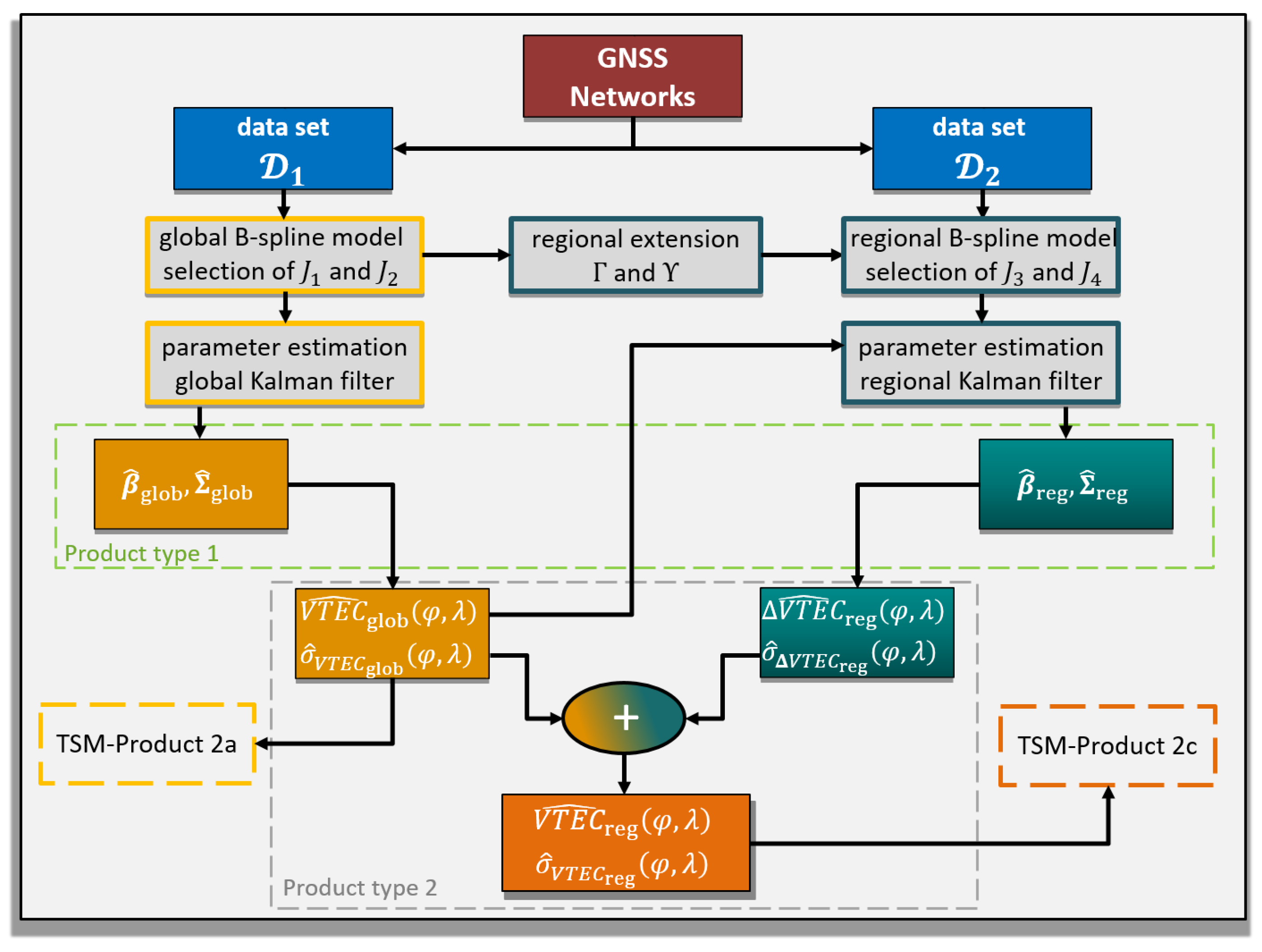
where the values ${\widehat{\sigma }}_{s,\mathrm{reg}}^2(\phi ,\lambda )$ and ${\widehat{\sigma }}_{s,\mathrm{glob}}^2(\phi ,\lambda )$ for each point $P(\phi ,\lambda )$ at time moments $t_s$ are given by the diagonal elements of ${\widehat{\mathsf{\Sigma }}}_{s,\mathrm{glob}}$ and ${\widehat{\mathsf{\Sigma }}}_{s,\mathrm{reg}}$, respectively. A flowchart of the developed TSM approach is shown in Figure 2. Starting from global and regional GNSS station networks, the respective data sets ${\mathcal{D}}_1$ and ${\mathcal{D}}_2$ are defined. The left side of Figure 2 depicts the process chain for generating the global model part. The right-hand side of the flowchart shows the process for generating the regional densification. Here the extent of the densification area has to be chosen in dependency of the global levels $J_1$ and $J_2$ according to (12). Furthermore, the global model is required as a background for modelling the regional $\mathsf{\Delta }VTEC$.

At the end of the process chain, the regional high-resolution $VTE{C}_{\mathrm{reg}}$ values are calculated by combining the estimated global and regional model parts according to the Equations (29) and (30).

VTEC Products

According to [9], the previously explained procedure allows for the dissemination of two types of products, namely

–

Product type 1:

a)

estimated B-spline coefficients ${\widehat{d}}_{k_1,k_2}^{J_1,J_2}\left(t_s\right)$ and their standard deviations ${\widehat{\sigma }}_{d,k_1,k_2}^{J_1,J_2}\left(t_s\right)$ for the global model of levels $J_1$ and $J_2$ at time moments $t_s$ as well as

b)

estimated B-spline coefficients ${\widehat{d}}_{k_3,k_4}^{J_3,J_4}\left(t_s\right)$ with their standard deviations ${\widehat{\sigma }}_{d,k_3,k_4}^{J_3,J_4}\left(t_s\right)$ for the regional model of levels $J_3$ and $J_4$ at time moments $t_s$ and

–

Product type 2

a)

estimated values ${\widehat{VTEC}}_{\mathrm{glob}}({\phi }_v,{\lambda }_v,t_s)$ and their standard deviations ${\widehat{\sigma }}_{VTE{C}_{\mathrm{glob}}}({\phi }_v,{\lambda }_v,t_s)$ on a regular grid of the global model at time moments $t_s$ taken from the Equations (25) and (26) as well as

b)

estimated values ${\widehat{\mathsf{\Delta }VTEC}}_{\mathrm{reg}}({\phi }_w,{\lambda }_w,t_s)$ and their standard deviations ${\widehat{\sigma }}_{\mathsf{\Delta }VTE{C}_{\mathrm{reg}}}({\phi }_w,{\lambda }_w,t_s)$ from Equation (29) on a regular grid of the regional model at time moments $t_s$ taken from the Equations (27) and (28) as well as

c)

estimated values ${\widehat{VTEC}}_{\mathrm{reg}}({\phi }_w,{\lambda }_w,t_s)$ and their standard deviation ${\widehat{\sigma }}_{VTEC,\mathrm{reg}}({\phi }_w,{\lambda }_w,t_s)$ on a regular grid of the regional model at time moments $t_s$ taken from the Equation (29) and (30)

to the user. The two product types reflect the two strategies of dissemination. In terms of product type 2, VTEC is provided to users typically by means of the IONEX format, see [18]. Thereby, the sampling intervals $\mathsf{\Delta }\mathsf{\Phi }$ in latitude and $\mathsf{\Delta }\mathsf{\Lambda }$ in longitude between the grid points $P({\phi }_v,{\lambda }_v)$ are usually chosen as $1^{°},{2.5}^{°}$ or $5^{°}$. For the calculation of VTEC values at arbitrary points between the grid points an interpolation has to be applied which generally degenerates the quality of the calculated values [9]. In the case of product type 1, the VTEC values and the corresponding standard deviations can be calculated at arbitrary points with higher accuracy using the Equations (25) to (28) directly. However, then an encoder procedure for the estimated B-spline coefficients is necessary. In fact, the presented two-step approach described in Section 2.1 provides two products in terms of Product type 2, namely

–

TSM-Product 2a

the global model $VTE{C}_{\mathrm{glob}}(\phi ,\lambda ,t)$ as well as the corresponding standard deviations ${\sigma }_{\mathrm{glob}}(\phi ,\lambda ,t)$ for the representation of VTEC on a global scale and

–

TSM-Product 2c

the regional model $VTE{C}_{\mathrm{reg}}(\phi ,\lambda ,t)$ and the corresponding standard deviations ${\sigma }_{\mathrm{reg}}(\phi ,\lambda ,t)$ for the representation of VTEC with a higher spatial and spectral resolution within the selected region.

Due to the independent estimation of the coefficients $d_{k_1,k_2}^{J_1,J_2}$ for the global and $d_{k_3,k_4}^{J_3,J_4}$ for the regional model part, the global model is not affected by the densification step and can be disseminated as Product type 2a. The second step of the TSM, however, depends on the global background model. Hence, in this case both model steps have to be evaluated in order to provide the TSM-Product type 2c.

3. Two-Step Model for Europe

In the sequel, the developed approach is applied to real data collected during March 2015. This time span is selected because of the solar storm, the St. Patrick storm, happened on March 17. Thus, stronger spatial variations in VTEC can be observed and modeled. We apply the TSM with a densification for the European region. It is particularly suitable for the application of the TSM due to a dense coverage of receiver stations from both, the global IGS network and the regional EUREF network, which provides a dense observation distribution over Europe, see Figure 1. It shall be noted that the idea of the following investigation is the generation of a VTEC model defined within a region that is characterized by a high spatial and spectral resolution such that a TSM-Product 2c can be established. It is not our objective to create a VTEC model of the most highest spatial and spectral content for a given region.

3.1. Global Model

We follow the workflow for the TSM procedure presented in Figure 2 and start with the definition of the different data sets ${\mathcal{D}}_1$ for the global modelling part. Figure 3 shows in the left-hand panel all available stations from the global IGS network (red dots) and from the regional open network in Europe, EUREF (blue dots). The right-hand panel depicts the selected stations for creating the set ${\mathcal{D}}_1$ with a more homogeneous distribution over the globe ${\mathsf{\Omega }}_H$. The stations are selected by means of a segmentation of the Earth’s surface into bins of size ${10}^{°}\times {10}^{°}$ w.r.t. latitude and longitude, according to the inequality chains (10).

The observations related to the IPPs of the chosen receiver stations define the data set ${\mathcal{D}}_1$. Figure 4 shows exemplarily the corresponding IPPs from GPS and GLONASS on 17 March 2015 at 12:00 UT with a less dense data coverage over the continental regions compared to the distribution of IPPs in Figure 1.

According to the workflow in Figure 2 (left), the next step is to select the global B-spline levels $J_1$ and $J_2$. As already mentioned in the context of Table 1 the levels $J_1=4$ and $J_2=3$ are chosen here. Given the vectors ${\mathit{y}}_{s,\mathrm{glob}}$, ${\mathit{e}}_{s,\mathrm{glob}}$, the matrices ${\mathsf{\Sigma }}_{y,\mathrm{glob}}$, ${\mathsf{\Sigma }}_{w,\mathrm{glob}}$, we run the Kalman filter for estimating the unknowns of the global model. We set the Kalman filter step size to $\mathsf{\Delta }t=t_s-t_{s-1}=10$ minutes and estimate the $18·24=432$ global B-spline coefficients as well as the the corresponding standard deviations

$$\begin{array}{c}\hfill {\widehat{d}}_{k_1,k_2}^{4,3}\left(t_s\right){|}_{k_1=0,\dots ,17,k_2=0,\dots ,23},\\ \hfill {\widehat{\sigma }}_{d,k_1,k_2}^{4,3}\left(t_s\right){|}_{k_1=0,\dots ,17,k_2=0,\dots ,23}\end{array}$$

(31)

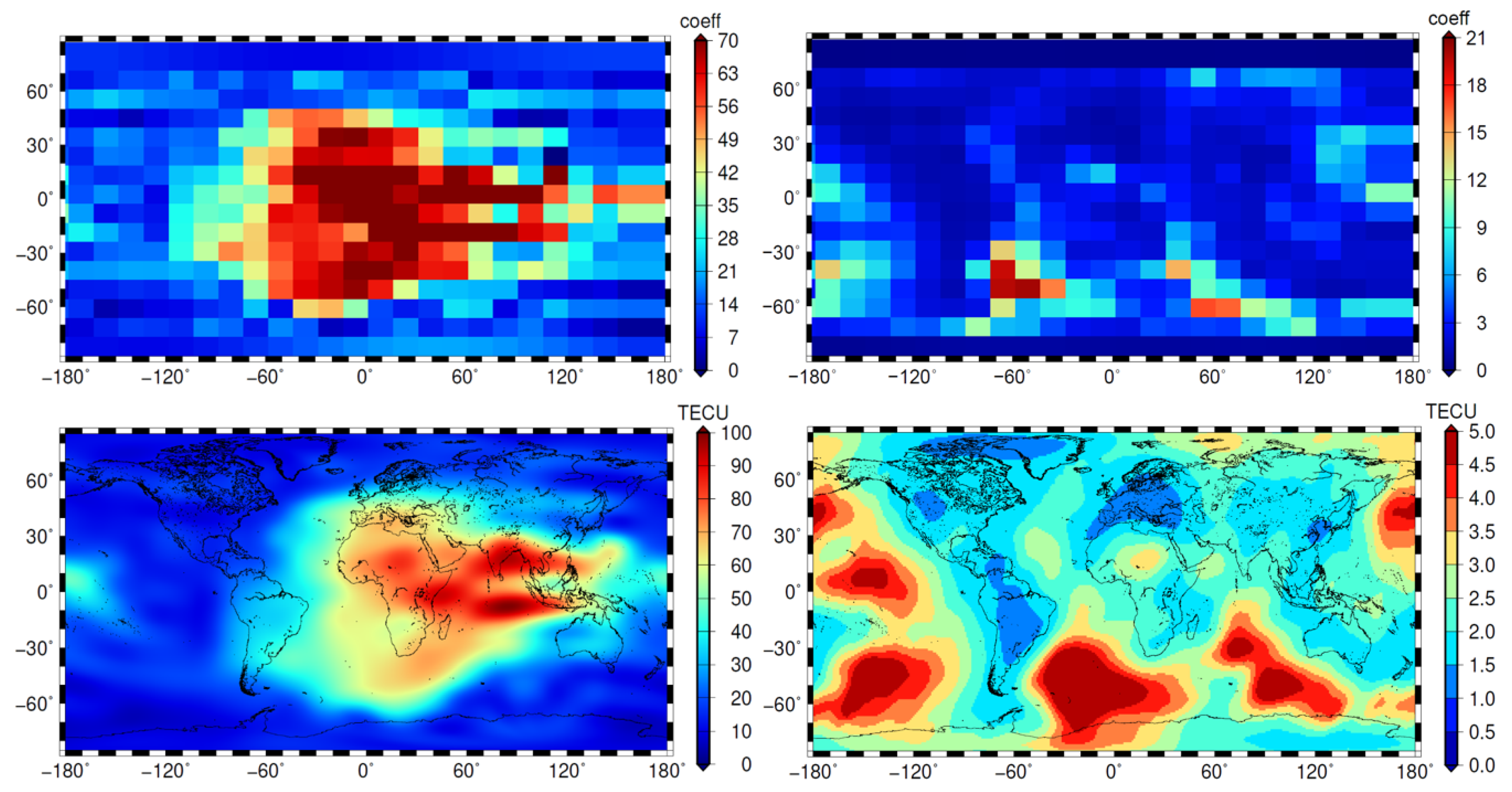
with $K_{J_1}=2^4+2=18$ and $K_{J_2}=3·2^3=24$. The top left panel of Figure 5 shows the estimated coefficients and the top right panel the corresponding standard deviations from the Equations (19) and (20), respectively.

The estimated parameters are of Product type 1a as defined in Section 2.3. For the calculation of Product type 2a we select the output sampling intervals $\mathsf{\Delta }\mathsf{\Phi }={2.5}^{°}$ and $\mathsf{\Delta }\mathsf{\Lambda }=5^{°}$ w.r.t. the geographical latitude and longitude, resp., as well as the temporal output sampling interval $\mathsf{\Delta }T=10$ minutes. The estimated grid values ${\widehat{VTEC}}_{\mathrm{glob}}({\phi }_v,{\lambda }_v,t_s)$ and the corresponding standard deviations ${\widehat{\sigma }}_{VTE{C}_{\mathrm{glob}}}({\phi }_v,{\lambda }_v,t_s)$ are shown in the lower panels of Figure 5. Note, here we applied a bi-linear interpolation according to [9,18] for visualization.

From the comparison of the two left-hand side panels, it can be stated that the numerical values of the estimated coefficients reflect the spatial signal structures in VTEC due to the localizing feature of the B-spline expansion. The standard deviations in the right-hand side panels reflect the data distribution. Hence, there are significantly larger standard deviations where only a few number of observations are available. This can be verified by comparing the standard deviations with the distribution of the IPPs shown in Figure 4.

3.2. Regional Model

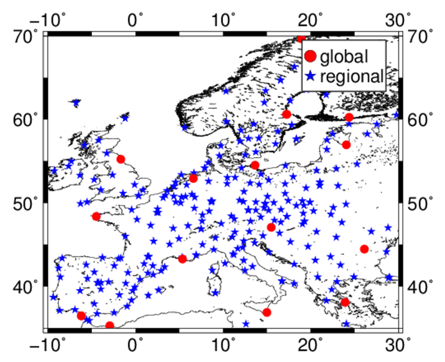
As with the modelling of the global part, the first step for the regional model is to define the data set $D_2$. The method for this has already been described at the end of Section 2.1. Figure 6 depicts the receiver stations for both data sets $D_1$ (red circles) and $D_2$ (blue stars) within the European region.

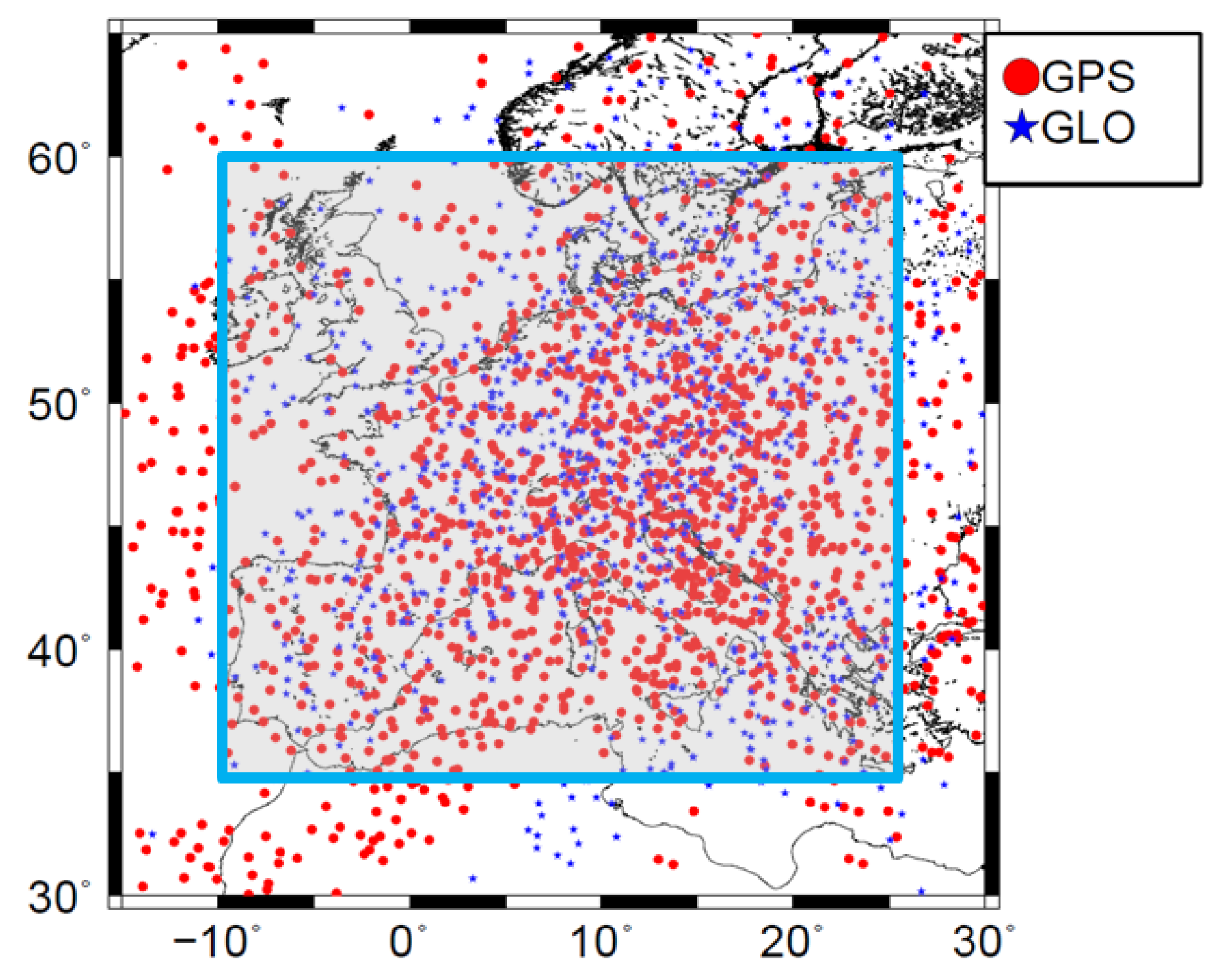
The observations related to the IPPs of the receiver stations within the regional densification area are collected in the data set ${\mathcal{D}}_2$ and exemplarily shown in Figure 7. Since the relation ${\mathcal{D}}_1\cap {\mathcal{D}}_2=\varnothing$ holds, no observation can be a member of both data sets. Consequently, we assume negligible correlations between the two data sets.

The regional model is set up after the definition of the size $\mathsf{\Delta }\mathsf{\Omega }$ of the densification area. According to the inequalities (12) and (13) the regional levels $J_3$ and $J_4$ have to be defined independence of the observation distribution over Europe. We proceed as follows:

• Selection of the regional extent
  According to (12) the minimum wavelength represented by the global model must fit into the region. With the chosen level values $J_1=4$ and $J_2=3$ we obtain from Table 1 $L_{\phi }={21}^{°}$ in latitude and $L_{\lambda }={30}^{°}$ in longitude. The most homogeneous and dense distribution of IPPs of the data set ${\mathcal{D}}_2$ is given between the latitudes $\phi \in [{35}^{°},{60}^{°}]$ and the longitudes $\lambda \in [-{10}^{°},{25}^{°}]$, this area is highlighted with the blue box in Figure 7. The densification area $\mathsf{\Delta }\mathsf{\Omega }$ is chosen accordingly with a extension of $\mathsf{{\rm Y}}={25}^{°}$ and $\mathsf{\Gamma }={35}^{°}$, and thus fulfills the requirement (12).
• Selection of the B-spline levels
  Although the sampling intervals in the center of the defined region $\mathsf{\Delta }\mathsf{\Omega }$ are particularly small, the average sampling intervals $\mathsf{\Delta }\phi \le {2.5}^{°}$ and $\mathsf{\Delta }\lambda \le {2.5}^{°}$ are chosen due to the larger gaps at the boundaries. Substituting $\mathsf{\Delta }\phi$, $\mathsf{\Delta }\lambda$, $\mathsf{{\rm Y}}$ and $\mathsf{\Gamma }$ in the mid part of the chain (13) yields the maximum B-spline levels $J_3=3$ and $J_4=3$ from Table 2 which shows the numbers from the inequality chains (13) analog to Table 1 for the global case.

From Table 1 we identified the global level values $J_1=4$ and $J_2=3$ with the SH degrees value $n_{max}=17$ and $n_{max}=12$, resp., as cutoff frequency of the spectral signal content of VTEC. From Table 2 we obtain in the same manner for the B-spline levels $J_3=3$ and $J_4=3$ of the regional model. Consequently, our final regional VTEC model contains apectral component up to the cutoff frequencies $n_{max}=64$ in latitude direction and $n_{max}=47$ in longitude direction.

With the chosen level values $J_3=3$, $J_4=3$, the observation vector ${\mathit{y}}_{s,\mathrm{reg}}$, the measurement error vector ${\mathit{e}}_{s,\mathrm{reg}}$, the covariance matrix ${\mathsf{\Sigma }}_{y,\mathrm{reg}}$ of the observations and the covariance matrix ${\mathsf{\Sigma }}_{w,\mathrm{reg}}$ of the process noise, we perform the estimation of the regional B-spline coefficients by means of the Kalman filter. Its step size is set to $\mathsf{\Delta }t=10$ minutes, as it was applied for the global model. We obtain the estimated coefficients and their standard deviations as

$$\begin{array}{c}\hfill {\widehat{d}}_{k_3,k_4}^{3,3}\left(t_s\right){|}_{k_3=0,\dots ,9,k_4=0,\dots ,9}\\ \hfill {\widehat{\sigma }}_{d,k_3,k_4}^{3,3}\left(t_s\right){|}_{k_3=0,\dots ,9,k_4=0,\dots ,9}\end{array}$$

(32)

with $K_{J_3}=2^3+2=10$ and $K_{J_4}=2^3+2=10$ as the total number of B-spline coefficients. As for the global model part a test of significance was carried out for the estimated coefficients. From the 100 B-spline coefficients around 60 to 70 are significant during night time and 70 to 75 at local noon, with a $\alpha$-value of 0.01. During the storm time on March 17, the number of significant coefficients increases to 80, because of the stronger signal variations during that time.

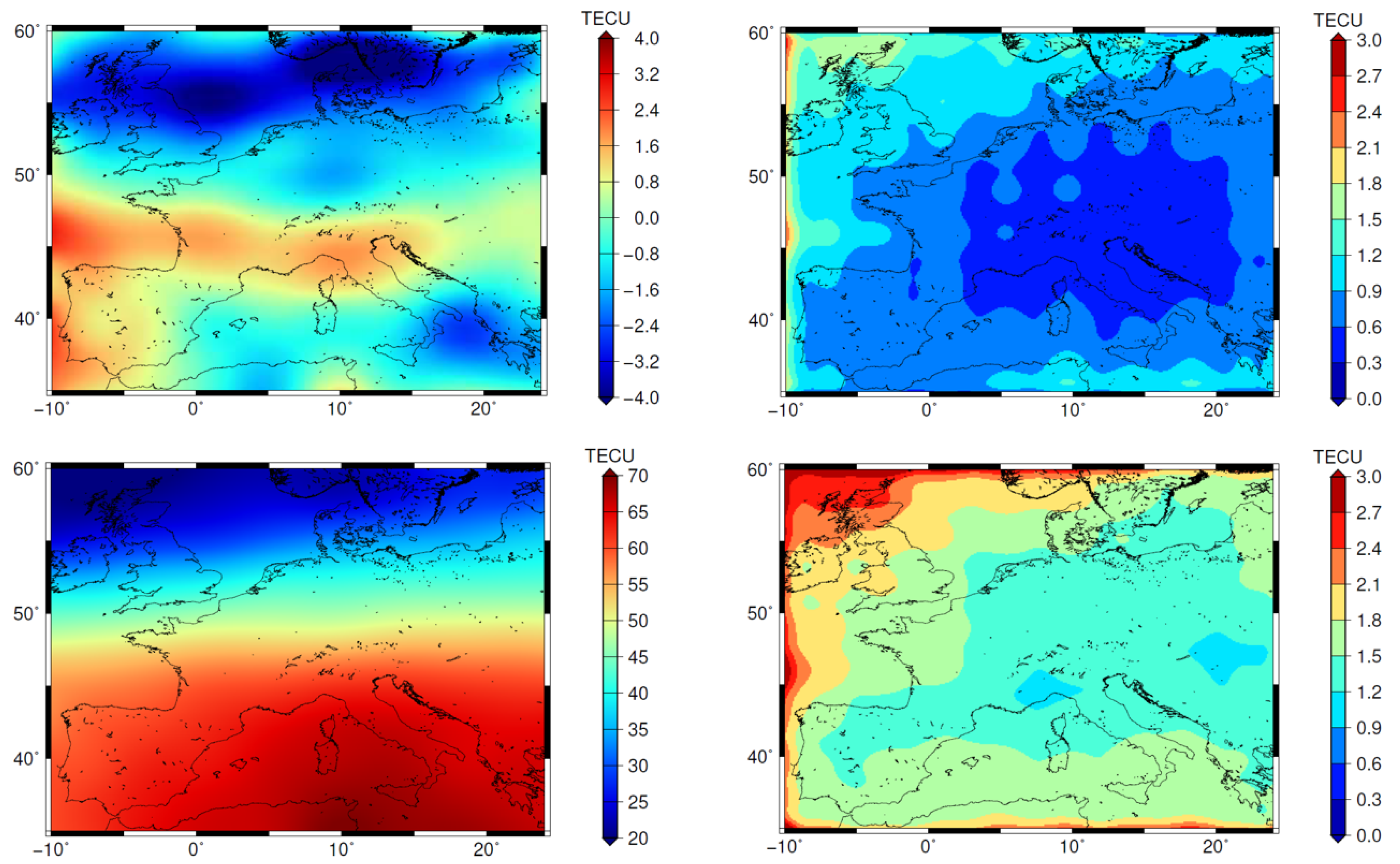
For the example in Figure 8, we applied the Equations (27) and (28) to calculate $\mathsf{\Delta }VTEC$ and their corresponding standard deviations on a grid as Product type 2b introduced in Section 2.3. We chose the output sampling intervals $\mathsf{\Delta }\mathsf{\Phi }=1^{°}$ in latitude and $\mathsf{\Delta }\mathsf{\Lambda }=1^{°}$ in longitude. For the representation of the map in the upper panels of Figure 8 we use the bi-linear interpolation [9].

For the calculation of the total VTEC values and the corresponding standard deviations within the region $\mathsf{\Delta }\mathsf{\Omega }$ we finally apply the Equations (29) and (30) using the estimated values – defined as Product type 2a – ${\widehat{VTEC}}_{\mathrm{glob}}(\phi ,\lambda ,t)$ and ${\widehat{\sigma }}_{VTE{C}_{\mathrm{glob}}}(\phi ,\lambda ,t)$ at the same grid points with sampling intervals $\mathsf{\Delta }\mathsf{\Phi }=1^{°}$ and $\mathsf{\Delta }\mathsf{\Lambda }=1^{°}$. The lower panels represent finally the maps of Product type 2c with ${\widehat{VTEC}}_{\mathrm{reg}}(\phi ,\lambda ,t)$ as the total VTEC values (left) and ${\widehat{\sigma }}_{VTE{C}_{\mathrm{reg}}}(\phi ,\lambda ,t)$, the corresponding standard deviations (right) within the European region for 17 March 2015 at 12:00 UT.

Due to the absolute magnitude of the global signal values with up to 120 TECU, the detailed structures of the regional model with magnitudes of ±4 TECU cannot be visualized appropriately in the bottom left panel of Figure 8. The standard deviation map on the bottom right panel shows larger values at the region boundaries and thus, reflects rather nicely the distribution of the observations, cf. Figure 4 and Figure 7.

4. Validation

In order to assess the VTEC TSM Products 2a and 2c as defined at the end of Section 2, we use the so-called dSTEC analysis. It is based on real GNSS observations for the comparison with the estimated VTEC maps and features an accuracy of less than 0.1 TECU, [8]. The differences

$$dSTE{C}_{obs}\left(t_s\right)=STEC({\mathit{x}}_s^S,{\mathit{x}}_{s,R},t_s)-STEC({\mathit{x}}_{ref}^S,{\mathit{x}}_{ref,R},t_{ref})$$

(33)

between the observations $STEC({\mathit{x}}_s^S,{\mathit{x}}_{s,R},t_s)$ according to Equation (2) at time moments $t_s$ and the observation $STEC({\mathit{x}}_{ref}^S,{\mathit{x}}_{ref,R},t_{ref})$ at the reference time moment $t_{ref}$ along the same arc is compared with the differences

$$dSTE{C}_{map}\left(t_s\right)=M\left(z_s\right)·VTEC({\mathit{x}}_{s,IPP},t_s)-M\left(z_{ref}\right)·VTEC({\mathit{x}}_{ref,IPP},t_{ref}),$$

(34)

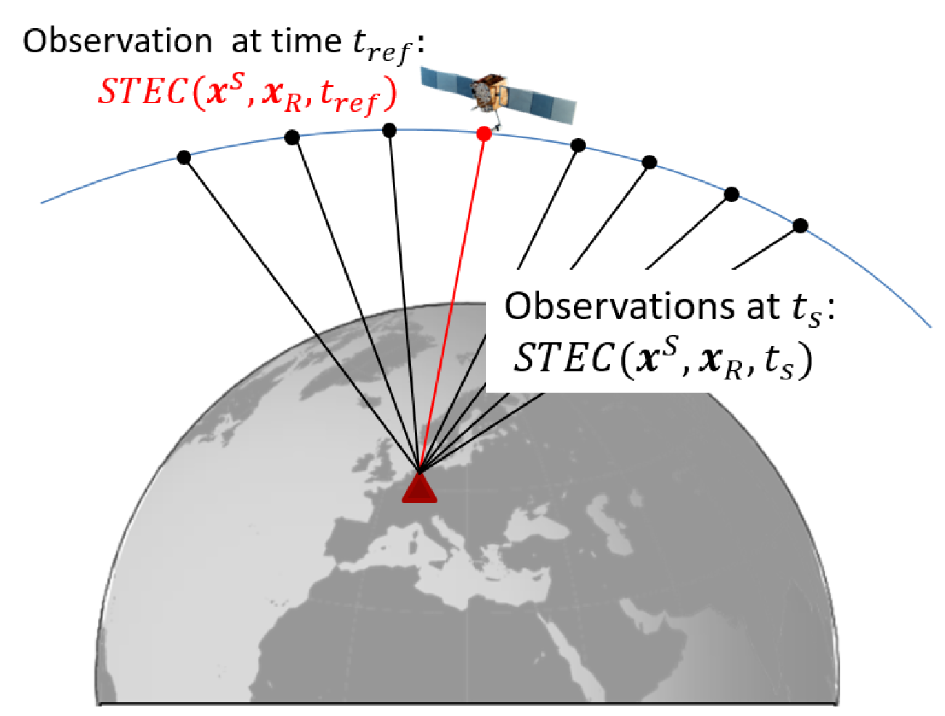
according to Equation (4). The reference time moment $t=t_{ref}$ is usually referred to the observation with the smallest zenith angle $z=z_{ref}$, see Figure 9. The quality assessment is finally performed by evaluating the differences

$$dSTEC\left(t_s\right)=dSTE{C}_{obs}\left(t_s\right)-dSTE{C}_{map}\left(t_s\right)$$

(35)

with expectation value $E\left(dSTEC\left(t_s\right)\right)=0$, for different products, e.g., the TSM-Products 2a and 2c, or the final GIMs of IGS [32], or its IAACs as it was done by Roma-Dollase et al. [7].

Within the dSTEC analysis the difference (35) has to be calculated for a set of a number of selected receiver stations. For the choice of the receiver stations three strategies exist:

• The observations of the selected receiver stations are used for the computation of all maps used in the analysis
• No station of the selected receivers stations contributed to any of the different products, thus, the stations are independent from all products
• A mixture of stations satisfying the items 1. and 2.

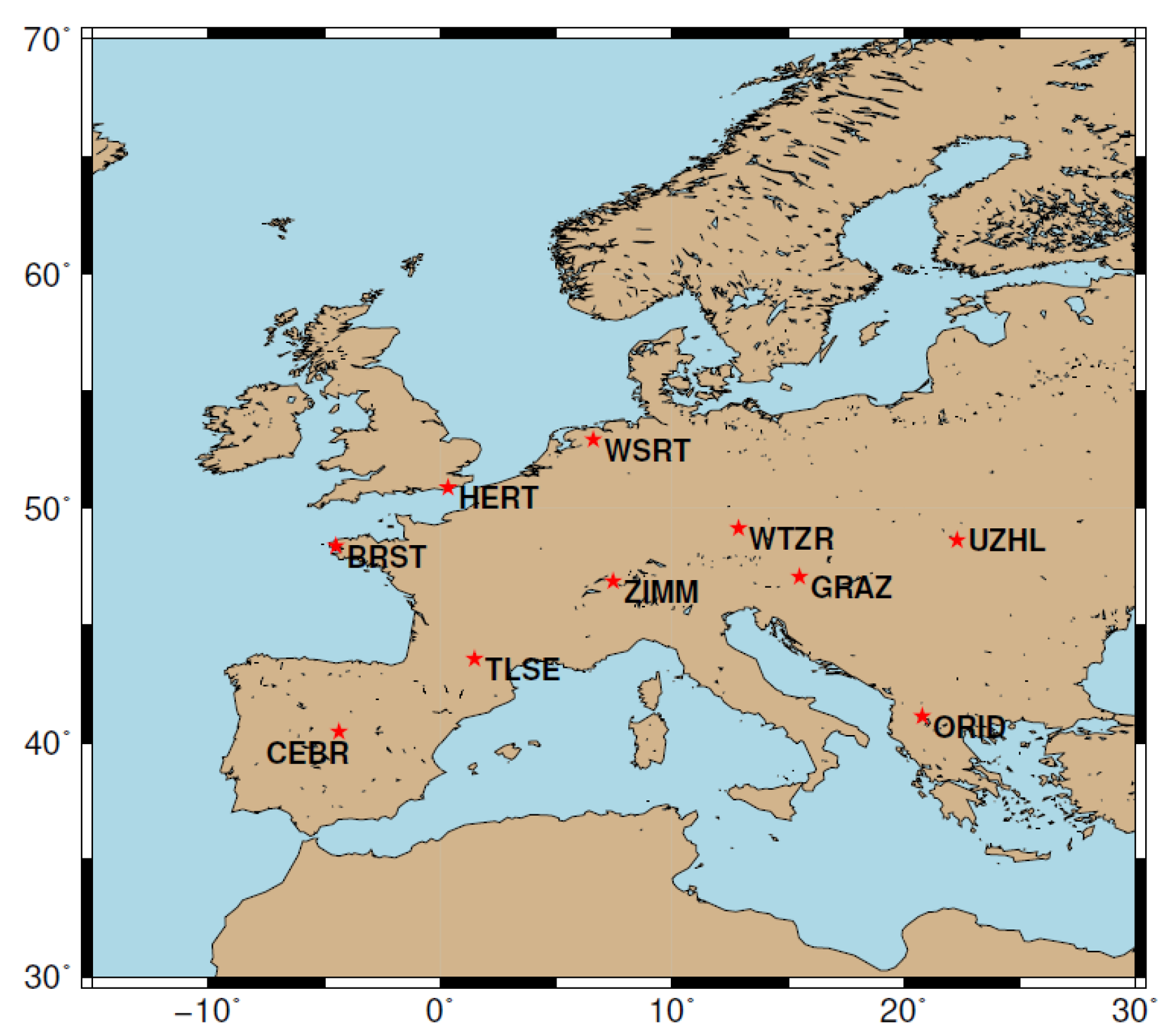
Since we define non-overlapping station lists providing observations to ${\mathcal{D}}_1$ and ${\mathcal{D}}_2$, we follow the third strategy. Figure 10 shows the stations used in our dSTEC analysis. Note, we selected also stations that are located close to the boundaries of the region, to use their observations with IPPs located within the region.

For the assessment of the product quality we use the following TSM-Products (cf. Goss et al. [9]):

 

TSM-Product 2a:

–

otlg_a:

the estimated ${\widehat{VTEC}}_{\mathrm{glob}}^{4,3}(\phi ,\lambda ,t)$ with a grid resolution of $\mathsf{\Delta }\mathsf{\Phi }={2.5}^{°}$, $\mathsf{\Delta }\mathsf{\Lambda }=5^{°}$ and $\mathsf{\Delta }T=10$ minutes temporal sampling interval

–

otlg_b:

the estimated ${\widehat{VTEC}}_{\mathrm{glob}}^{4,3}(\phi ,\lambda ,t)$ with a grid resolution of $\mathsf{\Delta }\mathsf{\Phi }=1^{°}$, $\mathsf{\Delta }\mathsf{\Lambda }=1^{°}$ and $\mathsf{\Delta }T=10$ minutes temporal sampling interval

 

TSM-Product 2c:

–

othr:

the estimated ${\widehat{VTEC}}_{\mathrm{reg}}^{3,3}(\phi ,\lambda ,t)$ with a grid resolution of $\mathsf{\Delta }\mathsf{\Phi }=1^{°}$, $\mathsf{\Delta }\mathsf{\Lambda }=1^{°}$ and $\mathsf{\Delta }T=10$ minutes temporal sampling interval.

We denote the global models as ‘otlg’ similar to Goss at al. [9]. The first letter ‘o’ refers to the OPTIMAP processing software, which was developed within a third-party project (see Acknowledgements) and means the basis of the presented study. The second letter indicates the chosen temporal output sampling interval with ‘t’ for $\mathsf{\Delta }T=10$ minutes. The third letter denotes the spectral content of the output signal; it is chosen as ‘h’ for high and ‘l’ for low. The last letter indicates the model domain with ‘g’ for global and ‘r’ for regional. In the case of the global model we indicate two different grid resolutions with their endings ‘a’ and ‘b’, cf.

Table 3. Products used for validation; names, types and latencies are taken from the references listed in the last column.

Institution	Product	Extension	Latency	$\mathsf{\Delta }\mathsf{\Phi }$	$\mathsf{\Delta }\mathsf{\Lambda }$	$\mathsf{\Delta }\mathit{T}$	Reference
DGFI-TUM	otlg_a	global	< 3 h	${2.5}^{°}$	$5^{°}$	10 min	[9]
DGFI-TUM	otlg_b	global	< 3 h	$1^{°}$	$1^{°}$	10 min	[9]
DGFI-TUM	othr	regional	< 3 h	$1^{°}$	$1^{°}$	10 min	this paper
ROB	robg	regional	> 1 week	${0.5}^{°}$	${0.5}^{°}$	15 min	[13,33]
CODE	codg	global	> 1 week	${2.5}^{°}$	$5^{°}$	1 h	[34]
UPC	uqrg	global	> 1 day	${2.5}^{°}$	$5^{°}$	15 min	[7]

.

For the validation of our TSM-Products we use other products listed in Table 3. They are characterized by different extents, latencies and output samplings $\mathsf{\Delta }\mathsf{\Phi }$, $\mathsf{\Delta }\mathsf{\Lambda }$ and $\mathsf{\Delta }T$. We compare the global products ‘otlg_a’, ‘otlg_b’, ‘codg’ and ‘uqrg’, where ‘otlg_a’ and ‘otlg_b’ are based on ultra-rapid orbits and hourly GNSS observations with a latency of less than 3 h [9]. The CODE product ‘codg’ is a final product and thus, based on post-processed data. UPC’s product, denoted as ‘uqrg’, is a rapid product and based on rapid GNSS data with a latency of approximately one day. Our regional product ‘othr’ is an ultra-rapid product, too. The only comparable external product for Europe is a final one provided by the Royal Observatory of Belgium (ROB) with a latency of approximately one week.

Figure 11 shows the RMS values of the differences (35) during the time span between 8 March and 23 March 2015 for each product at the 10 receiver stations shown in Figure 10.

The RMS values at the different stations vary approximately between 0.5 TECU and 0.9 TECU. Note, during the geomagnetic storm on March 17, the RMS values for all products at all stations increase and can reach values of up to 4 TECU for a short time, but are averaged in Figure 11. In order to rate the RMS values at different station and for the TSM products appropriately, we need to distinguish the stations used in the assessment, which are assigned either to ${\mathcal{D}}_1$ or to ${\mathcal{D}}_2$. Hence, the stations ‘BRST’, ‘HERT’, ‘GRAZ’, ‘WTZR’ and ‘WRST’ are stations which are used in the modelling procedure of the global VTEC maps, whereas ‘UZHL’, ‘ORID’, ‘CEBR’, ‘ZIMM’ and ‘TLSE’ are used for the regional model part. At a first step we compare the two global products of DGFI-TUM, ‘otlg_a’ and ‘otlg_b’ given with different spatial output sampling intervals $\mathsf{\Delta }\mathsf{\Phi }$ and $\mathsf{\Delta }\mathsf{\Lambda }$. Consequently, different RMS values are obtained for both products at all stations. For the values $VTEC({\mathit{x}}_{s,IPP},t_s)$ and $VTEC({\mathit{x}}_{ref,IPP},t_{ref})$ in Equation (34) a bi-linear interpolation has to be applied between the given grid points. The quality of the interpolated VTEC decreases with an increasing spatial resolution and thus, we achieve a slightly smaller overall RMS value for the product ‘otlg_b’. Comparing the bars for ‘otlg_a’ and ‘otlg_b’, we find larger differences in the RMS at the stations ‘UZHL’, ‘ORID’ and ‘CEBR’, which are independent stations for both models. The RMS values at all other stations are approximately equal.

In the next step, we compare the global product ‘otlg_b’ and the regional product ‘othr’. Both are given with the same spatial and temporal sampling intervals. From the orange colored and the red colored bars for ‘othr’ and ‘otlg_b’, respectively, we can conclude, that the regional model is of higher accuracy at all stations. This means, that we can achieve a significant improvement in the modelling accuracy within the region by applying the second step of the TSM. By comparing the overall RMS of ‘othr’ and ‘’otlg_b’, given in the parenthesis, we even find an increase in the accuracy of around $18.3$% for ‘othr’.

In order to rate the TSM-Products 2a against products of the IAACs, we compare the overall RMS values, of ‘otlg_a’ with 0.71 TECU, otlg_b’ with 0.70, ‘codg’ with 0.72 TECU and ‘uqrg’ with 0.76 TECU. Consequently, we find comparable results for the TSM products and ‘codg’ at all stations. However, when comparing the green and red color bars with the dark blue color bar for ‘codg’, for example at the stations ‘CEBR’ and ‘WTZR’, the differences are larger, so that local quality differences can be inferred. The product ‘uqrg’ performs slightly worse within the European region and for the selected time span, compared to the other global products.

Finally, we compare the regional TSM-Product 2b and the product ‘robg’. They are given with different spatial and temporal sampling, cf. Table 3, but the extension of the region covers with $\phi \in [{35}^{°},{60}^{°}]$ and $\lambda \in [-{10}^{°},{25}^{°}]$ for ‘othr’ and with $\phi \in [{35}^{°},{62}^{°}]$ and $\lambda \in [-{15}^{°},{25}^{°}]$ for ‘robr’ approximately the same area. However, ‘robg’ is a final product, whereas ‘othr’ is an ultra-rapid product. The product ‘othr’ shows a slightly higher accuracy than ‘robg’ of about 0.3 TECU in the overall RMS values. Nevertheless, both products are approximately of the same accuracy.

5. Summary and Conclusions

The presented approach aims at modelling VTEC with high spectral, spatial and temporal resolution for regions of dense data coverage. Compared to the GIMs provided by the IAACs, which are typically of lower spectral resolution, regional maps can represent finer structures. The global maps are usually provided with spatial output sampling intervals of $\mathsf{\Delta }\mathsf{\Phi }={2.5}^{°}$ and $\mathsf{\Delta }\mathsf{\Lambda }=5^{°}$ and a temporal sampling interval of $\mathsf{\Delta }T=2$ h. Regional maps, on the other hand, are usually provided with a finer grid resolution and a temporal sampling of $\mathsf{\Delta }T\le 1$ hour.

By means of the developed TSM, we generate both, a global model representing the coarser structures and a regional model representing the finer structures of VTEC. Both model parts are adapted optimally to the distribution of the independently defined data sets. The global data set consists of observations collected from selected receiver stations of the IGS network. To be more specific, the selection of these stations has to be adapted to the global situation. This means, that the observation sampling of the global data set has to fulfill the inequalities (10). Depending on the coverage the remaining receiver stations may provide dense clusters of observations within specific regions, cf. Figure 6. We performed numerical tests for Europe for March 2015, including the St-Patrick storm day, the strongest space weather event within the last decade. With the global resolution levels $J_1=4$ and $J_2=3$ we generate as the first step of the TSM the global VTEC model, comparable to the GIMs provided by the IAACs. In the second step, the regional VTEC model with resolution levels $J_3=3$ and $J_4=3$ is created. We apply the developed TSM to a densification area in Europe with cutoff frequencies of $n=64$ in latitude direction and $n=47$ in a longitude direction. Finally, the applied dSTEC validation shows that our generated regional ultra-rapid model with a latency of less than three hours is of higher accuracy than the global models and comparable to the regional final product of ROB.

Within this paper, we showed, that a higher spectral resolution and a higher accuracy can be achieved using appropriate regional modelling approaches. These high-resolution products can be used to study small scale and fast-changing variations of the ionosphere, e.g., traveling ionospheric disturbances (TID) [35,36], as well as plasma irregularities, such as plasma bubbles. For the use of the regional model in modern GNSS applications, such as autonomous driving or precision agriculture, the developed approach can be seen as an intermediate step towards the following developments:

–

Since autonomous driving or precise navigation requires real-time information about the state of the ionosphere, the TSM approach must be adapted accordingly. For this purpose, the latency (see Table 3) of the TSM products must be reduced significantly. There are two ways, namely (1) transferring the products to real-time using a suitable forecast algorithm or (2)—which is more preferably—directly applying real-time GNSS observations.

–

There is also the question of how ionosphere information should be disseminated to the user in real-time. In general, the dissemination can be undertaken in two different ways: based on estimated series coefficients (Products type 1) or on estimated grid values (Product type 2). In the latter case, an interpolation of the grid values has to be performed to obtain VTEC information at any arbitrary point within the area on the investigation. In case of dissemination of estimated series coefficients, the Radio Technical Commission for Maritime Services (RTCM) message has to be mentioned, which allows us to transfer of the SHs coefficients up to degree 16 to the user. It is in the current form restricted to the sole use of SHs and thus, not suitable for the high-resolution products developed within this paper. Consequently, the dissemination of the products needs to be discussed urgently in order to provide highly precise information to the users.

In a further step, a validation method for ionospheric maps will be developed that is more suitable for navigation applications. A more sophisticated method will allow the determination of positioning accuracy using ionospheric corrections from different products.

References

1. Langley, R.B. Propagation of the GPS Signals. In GPS for Geodesy; Teunissen, P.J.G., Kleusberg, A., Eds.; Springer: Berlin/Heidelberg, Germany, 1998; pp. 111–149. [Google Scholar] [CrossRef]
2. Schaer, S. Mapping and Predicting the Earth’s Ionosphere Using the Global Positioning System. Ph.D. Thesis, University of Bern, Bern, Switzerland, 1999. [Google Scholar]
3. Lyu, H.; Hernández-Pajares, M.; Nohutcu, M.; García-Rigo, A.; Zhang, H.; Liu, J. The Barcelona ionospheric mapping function (BIMF) and its application to northern mid-latitudes. GPS Solut. 2018, 22, 724–746. [Google Scholar] [CrossRef] [Green Version]
4. Hernández-Pajares, M.; Juan, J.M.; Sanz, J.; Argón-Àngel, A.; Garcia-Rigo, A.; Salazar, D.; Escudero, M. The ionosphere: Effects, GPS modeling and benefits for space geodetic techniques. J. Geod. 2011, 85, 887–907. [Google Scholar] [CrossRef]
5. Hernández-Pajares, M.; Juan, J.M.; Sanz, J.; Orus, R.; Garcia-Rigo, A.; Feltens, J.; Komjathy, A.; Schaer, S.C.; Krankowski, A. The IGS VTEC map: A reliable source of ionospheric information since 1998. J. Geod. 2009, 83, 263–275. [Google Scholar] [CrossRef]
6. Schmidt, M.; Dettmering, D.; Mößmer, M.; Wang, Y. Comparison of spherical harmonic and B-spline models for the vertical total electron content. Radio Sci. 2011, 46, RS0D11. [Google Scholar] [CrossRef]
7. Roma-Dollase, D.; Hernandez-Pajares, M.; Krankowski, A.; Kotulak, K.; Ghoddousi-Fard, R.; Yuan, Y.; Li, Z.; Zhang, H.; Shi, C.; Wang, C. Consistency of seven different GNSS global ionospheric mapping techniques during one solar cycle. J. Geod. 2018, 92, 691–706. [Google Scholar] [CrossRef] [Green Version]
8. Hernández-Pajares, M.; Roma-Dollase, D.; Krankowski, A.; García-Rigo, A.; Orús-Pérez, R. Methodology and consistency of slant and vertical assessments for ionospheric electron content models. J. Geod. 2017, 91, 1405–1414. [Google Scholar] [CrossRef]
9. Goss, A.; Schmidt, M.; Erdogan, E.; Görres, B.; Seitz, F. High-resolution vertical total electron content maps based on multi-scale B-spline representations. Ann. Geophys. 2019, 37, 699–717. [Google Scholar] [CrossRef] [Green Version]
10. Schmidt, M. Wavelet modelling in support of IRI. Adv. Space Res. 2007, 39, 932–940. [Google Scholar] [CrossRef]
11. Schmidt, M. Towards a multi-scale representation of multi-dimensional signals. In VII Hotine-Marussi Symposium on Mathematical Geodesy; Springer: Berlin/Heidelberg, Germany, 2012; Volume 137, pp. 119–127. [Google Scholar] [CrossRef]
12. Dettmering, D.; Schmidt, M.; Heinkelmann, R.; Seitz, M. Combination of different space–geodetic observations for regional ionosphere modeling. J. Geod. 2011, 85, 989–998. [Google Scholar] [CrossRef]
13. Bergeot, N.; Chevalier, J.M.; Bruyninx, C.; Pottiaux, E.; Aerts, W.; Baire, Q.; Legrand, J.; Defraigne, P.; Huang, W. Near real-time ionospheric monitoring over Europe at the Royal Observatory of Belgium using GNSS data. J. Space Weather Space Clim. 2014, 4, A31. [Google Scholar] [CrossRef] [Green Version]
14. Nohutcu, M.; Karslioglu, M.O.; Schmidt, M. B-spline modeling of VTEC over Turkey using GPS observations. J. Atmos. Sol. Terr. Phys. 2010, 72, 617–624. [Google Scholar] [CrossRef]
15. Liang, W. A Regional Physics-motivated Electron Density Model of the Ionosphere. Ph.D. Thesis, Technical University of Munich, Munich, Germany, 2017. Available online: http://mediatum.ub.tum.de/?id=1335966 (accessed on 24 March 2020).
16. Limberger, M. Ionosphere Modeling from GPS Radio Occultations and Complementary Data Based on B-splines. Ph.D. Thesis, Technical University of Munich, Munich, Germany, 2015. [Google Scholar]
17. Krypiak-Gregorczyk, A.; Wielgosz, P.; Borkowski, A. Ionosphere Model for European Region Based on Multi-GNSS Data and TPS Interpolation. Remote Sens. 2017, 9, 1221. [Google Scholar] [CrossRef] [Green Version]
18. Schaer, S.; Gurtner, W.; Feltens, J. IONEX: The IONosphere Map EXchange Format Version 1. In Proceedings of the IGS AC Workshop, Darmstadt, Germany, 9–11 February 1998. [Google Scholar]
19. Li, M.; Yuan, Y.; Wang, N.; Li, Z.; Zhang, X. Statistical comparison of various interpolation algorithms for reconstruction regional grid ionospheric maps over Cina. J. Atmos. Sol. Terr. Phys. 2018, 89, 331–345. [Google Scholar]
20. Lyche, T.; Schumaker, L. A mulitresolution tensor spline method for fitting functions on the sphere. SIAM J. Sci. Comput. 2001, 22, 724–746. [Google Scholar] [CrossRef] [Green Version]
21. Stollnitz, E.; DeRose, T.; Salesin, D. Wavelets for computer graphics: A primer, part I. IEEE Comput. Graph. Appl. 1995, 3, 76–84. [Google Scholar] [CrossRef]
22. Stollnitz, E.; DeRose, T.; Salesin, D. Wavelets for computer graphics: A primer. Part I and Part II. IEEE Comput. Graph. Appl. 1995, 15, 75–85. [Google Scholar] [CrossRef]
23. Schmidt, M.; Dettmering, D.; Seitz, F. Using B-Spline Expansions for Ionosphere Modeling; Springer: Berlin, Germany, 2015; Volume 89, pp. 939–983. [Google Scholar] [CrossRef]
24. Lee, J.; Kim, M. Optimized GNSS Station Selection to Support Long-Term Monitoring of Ionospheric Anomalies for Aircraft Landing Systems. IEEE 2017, 53, 236–246. [Google Scholar] [CrossRef]
25. Gelb, A. Applied Optimal Estimation; The MIT Press: Cambridge, MA, USA, 1974. [Google Scholar]
26. Grewal, M.S.; Andrews, A.P. Kalman Filtering: Theory and Practice Using MATLAB, 2nd ed.; John Wiley & Sons, Inc.: Hoboken, NJ, USA, 2008; p. 416. [Google Scholar]
27. Simon, D. A game theory approach to constrained minimax state estimation. IEEE Trans. Signal Process. 2006, 54, 405–412. [Google Scholar] [CrossRef] [Green Version]
28. Erdogan, E.; Schmidt, M.; Seitz, F.; Durmaz, M. Near real-time estimation of ionosphere vertical total electron content from GNSS satellites using B-spline in a Kalman Filter. Ann. Geophys. 2017, 35, 263–277. [Google Scholar] [CrossRef]
29. Laundal, K.M.; Richmond, A. Magnetic Coordinate Systems. Space Sci. Rev. 2016, 206, 27–59. [Google Scholar] [CrossRef] [Green Version]
30. Komjathy, A.; Langley, R. An assessment of predicted and measured ionospheric total electron content using a regional GPS network. In Proceedings of the 1996 National Technical Meeting of The Institude of Navigation; Institute of Navigation: Alexandria, VA, USA, 1996; pp. 615–624. [Google Scholar]
31. Erdogan, E.; Schmidt, M.; Goss, A.; Görres, B.; Seitz, F. Adaptive Modeling of the Global Ionosphere Vertical Total Electron Content. Geodyn. Model Dev. 2020. (close to submission). [Google Scholar]
32. Hernández-Pajares, M.; Juan, J.M.; Sanz, J. New approaches in global ionospheric determination using ground GPS data. J. Atmos. Sol. Terr. Phys. 1999, 61, 1237–1247. [Google Scholar] [CrossRef]
33. Bergeot, N.; Bruyninx, C.; Defraigne, P.; Pireaux, S.; Legrand, J.; Pottiaux, E.; Baire, Q. Impact of the Halloween 2003 ionospheric storm on kinematic GPS positioning in Europe. GPS Solut. 2011, 15, 171–180. [Google Scholar] [CrossRef]
34. Orus, R.; Cander, L.; Hernándes-Pajares, M. Testing regional vertical total electron content maps over Europe during 17–21 January 2005 sudden space weather event. Radio Sci. 2007, 42, RS3004. [Google Scholar] [CrossRef]
35. Yang, H.; Monte-Moreno, E.; Hernández-Pajares, M. Multi-TID detection and characterization in a dense Global Navigation Satellite System receiver network. J. Geophys. Res-Space 2017, 122, 9554–9575. [Google Scholar] [CrossRef]
36. Hernández-Pajares, M.; Wielgosz, P.; Paziewski, J.; Krypiak-Gregorczyk, A.; Krukowska, M.; Stepniak, K.; Kaplon, J.; Hadas, T.; Sosnica, K.; Bosy, J.; et al. Direct MSTID mitigation in precise GPS processing. Radio Sci. 2017, 52. [Google Scholar] [CrossRef] [Green Version]
Figure 1. Distribution of IPPs collected from stations of the IGS and the EUREF network on 17 March 2015 at 12:00 UT. Blue colored dots indicate observations from GPS, red colored dots from GLONASS.
Remotesensing 12 01198 g001
Figure 2. Flowchart of the two-step model (TSM), with the process chain for the first step—the global model—on the left side in yellow and the process chain for the second step—the regional densification—on the right side in green.
Remotesensing 12 01198 g002
Figure 3. Receiver stations of the global IGS network (red dots) and the European EUREF network (blue dots), left panel; selected receiver stations which provide observations for the global data set D 1 , right panel.
Remotesensing 12 01198 g003
Figure 4. Observation distribution of GPS and GLONASS observations on 17 March 2015 at 12:00 UT, from the global data set D 1 .
Remotesensing 12 01198 g004
Figure 5. Estimated coefficients (top left) and their standard deviations (top right) for the level values J 1 = 4 and J 2 = 3 within the GSM coordinate system; estimated vertical total electron content (VTEC) values (bottom left) and their standard deviations (bottom right) as GIMs defined in the geographical coordinate system; all sets calculated for 17 March 2015 at 12:00 UT.
Remotesensing 12 01198 g005
Figure 6. Receiver stations providing observations for the global data set D 1 (red dots) and stations providing observations for the regional data set D 2 (blue) within the European region.
Remotesensing 12 01198 g006
Figure 7. Distribution of the IPPs of the GPS and GLONASS observations from 17 March 2015 at 12:00 UT; the IPPs within the blue box are selected for the regional data set D 2 .
Remotesensing 12 01198 g007
Figure 8. Estimated Δ V T E C reg values and their standard deviations (upper panels) for the selected B-spline levels J 3 = 3 and J 4 = 3 ; estimated V T E C reg values (bottom left) and the corresponding standard deviation map (bottom right); all sets calculated for 17 March 2015 at 12:00 UT.
Remotesensing 12 01198 g008
Figure 9. Schematic representation of the dSTEC analysis of one satellite-receiver pair.
Remotesensing 12 01198 g009
Figure 10. Distribution of 10 receiver stations within the densification area used for the dSTEC analysis.
Remotesensing 12 01198 g010
Figure 11. RMS values computed at the 10 stations shown in Figure 10 for the products listed in the legend; the two global products ‘otlg_a’ and ‘otlg_b’ as well as the regional product ‘othr’, the external regional product ‘robg’ and the external global products ‘codg’ and ‘uqrg’ of the IAACs CODE and UPC are used for comparison. The values in the parantheses are the average RMS values over all 10 receiver stations for the entire test period between 8 March and 23 March 2015.
Remotesensing 12 01198 g011