An Automatic Method for Black Margin Elimination of Sentinel-1A Images over Antarctica


1
Center for Global Sea Level Change, New York University Abu Dhabi, Abu Dhabi 129188, UAE
2
Courant Institute of Mathematical Sciences, New York University, New York, NY 10012, USA
*
Author to whom correspondence should be addressed.
Remote Sens. 2020, 12(7), 1175; https://doi.org/10.3390/rs12071175
Submission received: 4 March 2020
/
Revised: 1 April 2020
/
Accepted: 1 April 2020
/
Published: 6 April 2020
(This article belongs to the Section Environmental Remote Sensing)
Abstract
:The Sentinel-1A satellite was launched in April 2014 with a primary C-Band terrain observation with progressive scans synthetic aperture radar (TOPSAR) onboard and has collected plenty of high-quality images for global change studies. However, low magnitude signals around image margins (black margins) does not preserve the normal standard level, influencing the potential usage with these data. Through image analysis, we find that the signal from black margin (BM) is highly dominated by the closest effective signals and the signal in BM shows an increasing trend along the direction from image boundary to image center. An edge detector is developed based on the signal characteristics of BM. Furthermore, an automatic method to discriminate and eliminate BM is designed. Images from both extra wide (EW) and interferometric wide (IW) swath observation modes, covering the land, ocean, and coast of the Antarctic, are taken to verify the robustness of our method. Through comparison with BM edges extracted by human interpretation, our method has the maximum BM edge extraction error of 1.9 ± 3.2 pixels. When considering perimeter (or area) difference along radial direction of BM edge, our method has an averaging extraction accuracy of −0.35 ± 0.11 (or 0.14 ± 1.38) pixels, which suggests that our method is effective and can be potentially used to eliminate BM for multidisciplinary applications of Sentinel-1 data.
1. Introduction
With the development of science and technology and the requirement for global environment change studies, a large quantity of satellites, from both optical and microwave remote sensing, have been launched to observe the rapid change of the Earth. Compared with previously launched satellites, modern satellites usually generate higher quality images with finer resolution. However, because of senor problem caused by equipment overuse, failure, or sensor design problems [1], satellites can sometimes obtain some poor quality data, such as data gaps or noisy pixels in an image, which may degrade the data quality and affects the wide use of these data in Earth science applications.
For optical remote sensors, Landsat-7 has experienced an image anomaly, or data gaps, because of the failure of the scan line corrector (SLC) after 31 May 2003 [2,3,4,5]. This malfunction of the SLC mirror led to abnormal data gaps in each images, covering almost 22% of the entire scanning area [6]. Additionally, the optical sensor of Landsat-7 may become saturated when scanning highly reflective land surface, such as snow or ice [7,8], making it difficult to inverse meaningful reflectance products by using the digital number directly. For microwave remote sensing satellites, especially synthetic aperture radar (SAR), the image analysis in land cover/change application is restricted by some low-quality images due to high backscatter noise, large signal ambiguity, saturation, and data gaps [1]. For instance, azimuth and range ambiguity is always challenging for ship detection with SAR images [9], which is caused by strong backscattered targets and sensor design problems. Besides of equipment design problems, some SAR images may contain large portion of data gaps (parallel black stripes) when the satellite sensor was overused, for example, some data gaps in Envisat-ASAR images [1]. Those poor-quality images from remote sensing satellite, regardless of whether they are from optical or microwave remote sensing, are difficult to use for different Earth science applications.
The recently launched Sentinel-1A has good image quality and its performance in most aspects is in line with expectation. The geolocation accuracy and performance in quantization, radiometric accuracy, resolution, and ambiguity of Sentinel-1A has been evaluated by [10,11,12,13,14]. However, along the different margins of an images of Sentinel-1A, poor-quality data (not always zero) does exist. In this paper, we call these poor-quality data black margin (BM) which corresponds to low signal magnitude and presents the black color around image margins. The boundary of BM is not provided with data images when being released and how to effectively extract the BM boundary is a challenging problem. This problem has been raised and discussed in the Science Toolbox Exploitation Platform forum [15] many times, but has not been completely solved. Without eliminating these black margins, poor results may be generated for image mosaic, co-registration, classification, and segmentation, restricting the multidisciplinary applications of Sentinel images, especially when the study area can only be covered by several different images. To expand the usage of Sentinel-1A images, especially for those using Level-1 data directly, an automatic method to identify and eliminate the BM along image boundaries is urgently required.
2. Sentinel-1A
Sentinel-1A, a carryon satellite following the ERS-1/2 and Envisat mission, is the first satellite from the Global Monitoring for Environment and Security (GMES) space component program, which was launched on 03 April 2014 by the European Space Agency (ESA) [16,17,18,19]. Sentinel-1A operates in a near polar and sun-synchronous orbit which is about 693 km above the ground [18,19] and has a repeat cycle of 12 days [20]. With a primary payload, the C-band terrain observation with progressive scans SAR (TOPSAR) [21] onboard, the primary scientific objective of Sentinel-1A is to observe ice changes in Arctic and Antarctic coastal regions as well as to monitor land changes, vessel, and oil spill in coastal regions [13,17,18,19,22]. Because Sentinel-1A is a C-band right-looking SAR, it has an advantage of observing the Earth in almost all weather conditions.
Sentinel-1A has the capability to collect measurements with dual (VV + VH or HH + HV) and single polarization (HH or VV) over global land or oceans. It adopts four different observation modes: interferometric wide (IW) swath mode, extra wide (EW) swath mode, strip map (SM) mode, and wave mode (WM) to monitor Earth changes at resolutions of 5 m × 20 m, 20 m × 40 m, 5 m × 5 m, and 5 m × 20 m respectively [18,19]. The four different observation modes are adopted according to different ground segments, which is subject to being changed from time to time. The images from different observation modes are processed, and four different Sentinel-1A products are provided according to different processing levels, which are SAR Level-0, Level-1 single look complex (SLC), Level-1 ground range detected (GRD), and Level-2 ocean (OCN) data. The Level-1 GRD data are produced after focusing, multi-looking, and being projected to a ground range using Earth ellipsoid model WGS-84 [17] and the Level-1 GRD data are usually suitable for most users if not doing SAR interferometry, especially for those working in land use/cover changes or image classification.
Since its launch in 2014, Sentinel-1A has demonstrated its promise in various applications, such as ocean wave height estimates [23], emergency event response [24,25], land change detection [26,27], sea ice drifting [28], ship detection [1,29,30], and glacier flow monitoring [31]. Over Antarctica, it provides good coverage and can collect repeated measurements in about 12 days with EW and IW observation modes. The spatial coverage of EW and IW GRD images over Antarctica during the entire month of May 2015 is shown in Figure 1. For each image, the quality and resolution of the Sentinel-1A data are good. However, along the image margins, poor-quality data do exist (Figure 2), which potentially restricts its applications in studies of large regions.
3. Backscatter Characteristics of Antarctic Land Surfaces
There are five typical land covers over the Antarctica ice sheet and the surrounding ocean: snow and land ice, rock, sea ice, ocean water, and icebergs. Snow and land ice covers most of the Antarctic ice sheet [7,32,33], and the surface layer can be penetrated to some extent [34] by Sentinel-1A (C-band SAR). The emitted radar signal is usually backscattered from some internal layer of snow. Therefore, the backscattered radar signal from snow and land ice is determined by dielectric properties, snow grain size, the number of internal reflectors, and the wetness of snow [35,36]. Rock takes only about 0.5 percent of the Antarctica ice sheet [32], but the backscattered radar signal from rock is complicated, depending on the corner reflectors and the surface facing the sensor. Icebergs are calved from land ice or ice shelves, and usually have a flat surface when drifting in the ocean. The backscattered radar signal is usually high because of strong volume scattering of surface snow layers. Sea ice can cover the Antarctica ocean seasonally and interannually, and the extent of sea ice varies with local wind speed and wind directions. Since most of sea ice is flat, the backscattered radar signal from sea ice is usually low. Similar to sea ice, the backscattered radar signal from ocean water is low because of the flat surface and right-looking nature of Sentinel-1A.
The backscattering character of different land cover in a SAR image is determined not only by different land cover but also the surface roughness of the land cover, facing slope of the land surface, and the range distance to the sensor. Land surface facing a SAR sensor usually results in great reflection of the emitted radar signal which acts as high backscatter in a SAR image or, inversely, low backscatter or radar shadow. Because of the different facing angle and surface roughness of different land covers, the backscattering of different land covers can present similar characteristics for some pixels. In spite of this, a homogenous region can always be detected in a SAR image as a result of the continuity of land surface morphology changes.
4. Edge Detector
Edge detection, especially step edge detection, is a typical requirement for image processing [37,38]. To extract edges effectively, multiple approaches have been developed, such as Roberts operator designed by [39], Sobel detector designed by [40], Prewitt operator designed by [41], Laplacian of Gaussian (LoG) operator designed by [42], and Canny operator designed by [37]. Most methods developed for edge detection are based on the first and the second derivative properties of an image. The first derivative operator defines the edge as local maximum of an image which convolves with the edge detector and the second derivative operator defines the edge as locations where the second derivative of an image crosses zero. Although the edge detectors were not designed for BM detection of Sentinel-1A, the idea of how to determine an edge can potentially contribute to BM detection and the image gradient between abnormal and effective signal is critical to edge detection of Sentinel-1A GRD data.
In this paper, we try to detect the edge between effective and abnormal signal in order to build a BM mask for each Sentinel-1A GRD image. A Sentinel-1A GRD image ‘s1a-ew-grd-hh-20151203t152802-20151203t152906-008879-00cb1d-001.tiff’ is taken as an example and Figure 2 shows its footprint around the Antarctic coast, which covers almost all different types of BMs. Figure 3 shows statistics of several image patches (10 × 15 pixels) from BM to effective signals, which suggests that signals from BM do not usually follow a normal distribution. However, for effective signals backscattered from land surface, one image patch from a homogeneous land surface following a normal distribution can always exist. According to these quite opposite properties, we design an edge detector to identify BM and the region of abnormal signal as follows.
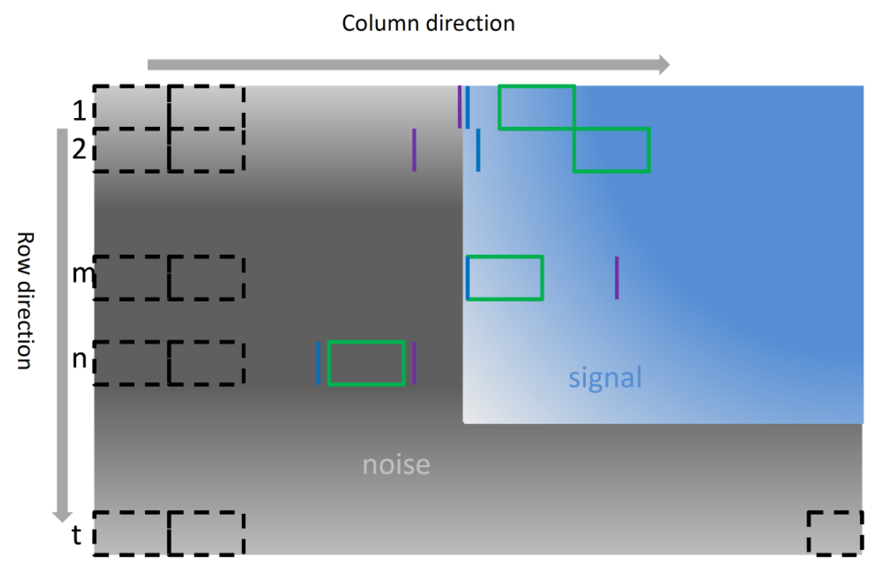
The edge is detected along the direction from the image boundary to the image center (which we henceforth refer to as the BC direction) from four different sides (the top, bottom, left, and right) and digital number (DN) for each pixel is used. Here, we will describe our method by taking the left side as an example. The same process can be applied to the other three sides. We define each 10 rows of a DN record as a searching unit, as can be seen from Figure 4 (i.e., 1, 2, …, m, n, t). A searching unit is composed of many image patches. In this paper, the image patch is set as 10 × 15 pixels.
Firstly, a coarse edge location (column number) is determined as a starting location of image patch ‘’, which is the first patch (at a size of 10 × 15 pixels) following normal distribution along the BC direction for each searching unit (Equation (1)). The normal distribution test is performed using the method proposed by [43] with the assumption that the mean and standard deviation are the same as that of the searching image patch. The edge location is defined as the column number, at least 80% of whose measurements are larger than a threshold ‘T’ along the BC direction. The threshold ‘T’ is defined by Equation (2). The edge starting location derived in this step is named as Edge Type 1 (ET1).
where ‘P’ is an image patch, ‘i’ is the ith searching unit, ‘j’ is the jth patch in this unit, stands for a normal distribution with mean of φ and standard deviation of σ, ‘T’ is the threshold, and ‘max’ means the operation to obtain the larger number of the two variables.
T = max(10, φ − 3σ)
Secondly, signal magnitude (DN value) for each searching unit is summed along the BC direction. However, only pixels from the beginning to the jth patch ‘’ which are detected from the first step are used. As a result, a one-dimensional vector along the BC direction is obtained. In order to detect edges starting from the first pixel along the BC direction, zero is usually inserted to the left of this vector. Then, the column number with the maximum gradient change is recorded and named as edge type 2 (ET2).
Thirdly, BM edge extraction. The BM edge in the column direction is determined as ET1 if the difference of ET1 and ET2 for each searching unit is less than a threshold ‘’ (Equation (3)). We call this part of ET1 as edge type (ET). From the sketch examples shown in Figure 4, we find some bad BM edge detection results from searching unit ‘2’, ‘m’, and ‘n’ and a good result from searching unit ‘1’.
where ‘i’ is the ith searching unit. ‘’ is a threshold, which is set as 3 pixels in this paper.
5. Method to Extract BM Edges
To obtain the complete edge of BM and effective signal for each Sentinel-1A images, four different sides (the top, bottom, left, and right) are processed separately. Since the edge should be close to the image boundary, only data within a certain distance to the four boundaries are processed. In this paper, we set this distance as 4000 pixels in the row (for the left and right) or column (for the top and bottom) direction to save computation costs. To better demonstrate this method, the left side is also taken as an example. The full process of BM edge extraction for the left side is described as follows, and the flowchart for processing is shown in Figure 5.
The first step is to extract accurate BM edges. The left section of the image examples with 4000 columns is selected first, and the BM edge is detected from the left to the right. Then ‘ET1’ and ‘ET2’ are obtained using the edge detector from Section 3. Meanwhile, the starting and ending row number of each searching unit are also recorded. ‘ET’ is obtained and smoothed using a median filter to exclude abnormal edge results.
The second step is to enrich edge location dataset. ET data from the edge detector has high accuracy, but may only correspond to some searching units. However, ET data can provide a reference for BM edge extraction for the remaining searching units. Since the BM edge from adjacent searching units should have similarity, edges with location difference, in a mathematic form of (ET1 − ET) smaller than a threshold, can be taken to enrich the edge datasets. Specifically, for each searching unit whose edge belongs to (ET1 − ET), the nearest searching unit whose edge belongs to ET from both unit increasing and decreasing directions will be found. Then, the slope of edge location versus searching unit number is calculated with Equation (4).
where stands for edge location of the mth searching unit from dataset (ET1 − ET) and ‘m’ has two different values ‘1’ and ‘2’.
If the slope from either side fulfills an equation, Equation (5), in which a threshold ‘’ is introduced, the corresponding edge location will be taken to enrich ET. We use ‘’ and ‘’ to stand for the nearest searching unit in column with increasing and decreasing direction, respectively.
where ‘’ and ‘’ are slopes of edge location versus unit number from unit increasing and decreasing direction respectively, ‘’ is the threshold, which is set as ‘ = 2’ here.
The third step is to detect the edge jump along different searching units and interpolate missing edges in column direction. The adjacent edge should be similar to each other if the searching unit is located in the same sub-swath, but the edge jump does exist because of different observing geometry of different sub-swaths, as can be seen from ‘1’ to ‘5’ from Figure 2. The edge step is determined by the difference of each of the two adjacent edges and only edge differences greater than ‘4’ pixels are discriminated as edge jumps. The missing edge for each searching unit is interpolated linearly using edge data before the edge jump. In this way, the edge accuracy is related to the size of the image patch—about 10 pixels.
The fourth step is to determine the edge jump to an accuracy of one pixel. The exact edge jump location is determined as the largest image gradient between two searching units around the edge jump in the row direction. The edge location for each unit close to the edge jump is re-interpolated with edges after the second step. Since the edge jump in the row is determined, the starting and ending row location of the processing unit including this edge jump can be revised.
In the last step, data gap extraction and BM mask generation. With BM edges and the starting and ending row number for each processing, the BM edge for left side can be built for each row. BM edges from the other three sides can also be extracted following the steps described above. A gap mask with a magnitude of zero is extracted as well and the union of gap mask and BM mask being calculated as a mask of final BM.
6. Results and Validation
The BM edges extracted with our algorithm, corresponding to four different boundaries (the top, bottom, left, and right) of the testing image can be found in Figure 6. Additionally, the BM edge is also extracted using the human interpretation method l (Figure 6e). Using human interpretation results as the reference, the BM edge was compared by traversal of all edge locations along four borders to check the difference of the edge location extracted from our method and human interpretation. Through calculating the difference of both results, the performance of our method was evaluated. The comparison results of edge location have a unit of pixel which can be easily converted to distance by multiplying with ground resolution of Sentinel-1A. Statistics of the difference of BM edge along all four borders were calculated.
Three indices for results comparison are introduced in this paper. The first one is the maximum difference along radial direction of BM. This index reflects the poorest results on edge extraction. ‘’, ‘’,’’, and ’’ stand for the maximum extraction error of edge on the left, right, top, and bottom boundary, respectively, as can be seen from Table 1.
The other two indices are the averaged edge error measured in pixel along radial direction of BM edge. Because BM extraction with different methods will have different perimeter and area, the BM edge extraction accuracy can be obtained by calculating equivalent pixel differences along the radial direction of BM when assuming the extraction error in perimeter and area are evenly distributed along the BM edge. The edge extraction error from both perimeter and area difference can be obtained through Equations (6) and (7).
where ‘’ and ‘’ is the area of the effective signal extracted from human interpretation and algorithm, respectively; ‘’ and ‘’ is the perimeter of effective signal region extracted from human interpretation and algorithm, respectively; ‘’ and ‘’ stand for average differences in the area and perimeter of effective signal regions, respectively; and ‘L’ is the resolution of each pixel.
The extraction results of BM edge and its comparison to that from human interpretation is shown in Figure 6. The maximum edge extraction error can reach 4, 4, 5, and 0 pixels for the left, right, top and bottom boundaries, respectively. Several typical mismatches of BM edge are shown in Figure 6e, marked from ‘A’ to ‘G’, zooming in of which is also embedded. On average, the BM edge extracted with our method coincides well with that from human interpretation. Most of large edge bias is concentrated in conjunctions of different edge steps.
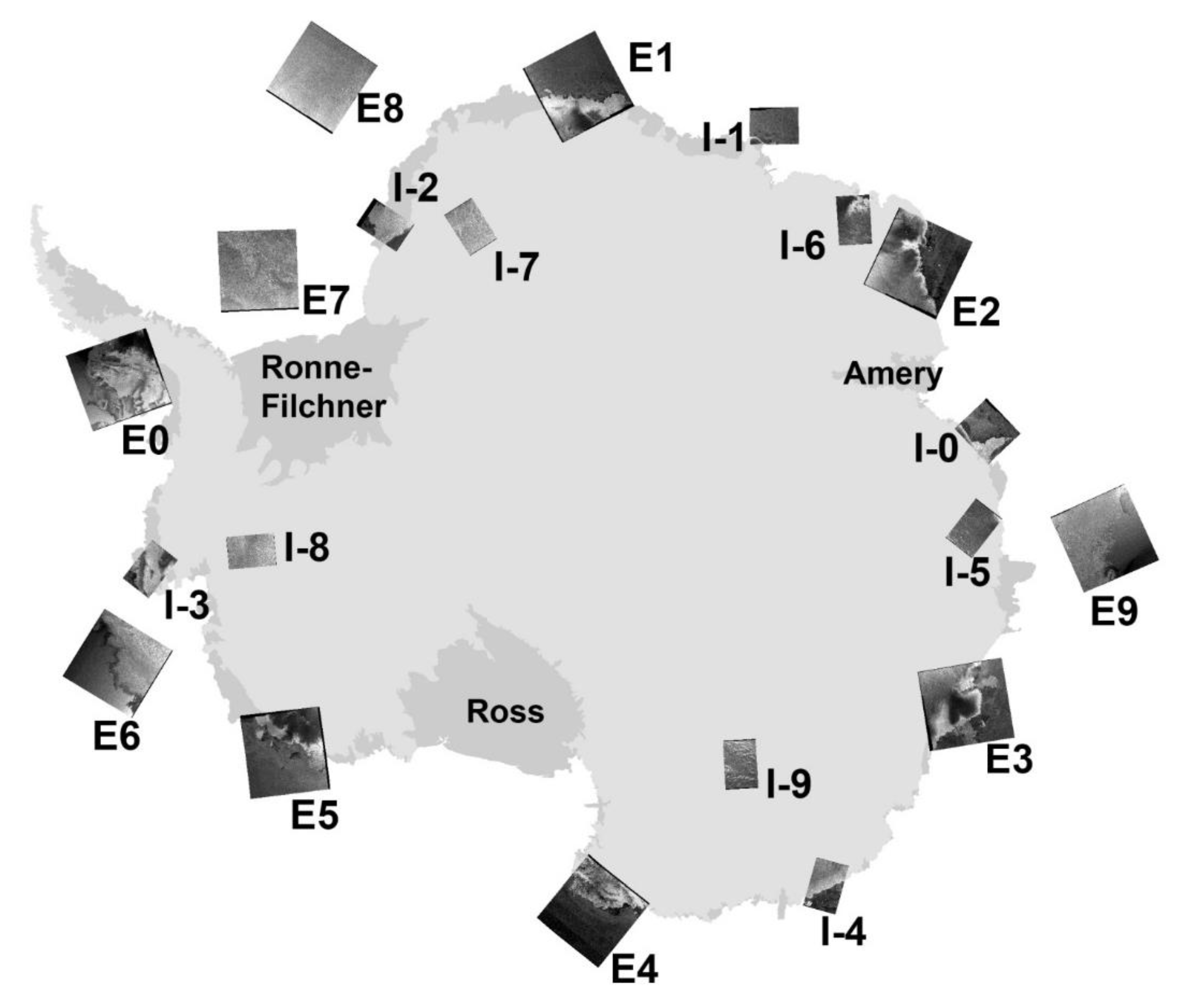
To further validate our algorithm, 20 Sentinel-1A GRD images from both EW and IW modes covering Antarctic land, coast, and ocean were selected for testing. Information of these 20 images can be found in Table 1 and their spatial coverage around Antarctica is shown in Figure 7. Six images (indices from E0 to E5) from Sentinel-1A EW mode cover the Antarctic coast and the other four images (indices from E6 to E9) cover the ocean surface around Antarctica. Five images (indices from I-0 to I-4) from Sentinel-1A IW mode cover Antarctic coast and the other five images (indices from I-5 to I-9) cover Antarctic inland. These images distribute evenly and cover all different land cover of Antarctica. The edge extraction results can be found in Supplementary Figures S1–S20.
From Table 1, the results from our algorithm have good accuracy, on average, with a maximum edge extraction error of 1.9 ± 3.2 pixels. Considering all 20 Sentinel-1A GRD images, the edge extraction accuracy is −0.35 ± 0.11 and 0.14 ± 1.38 pixels when considering perimeter and area difference, respectively.
7. Discussions
7.1. BM Edge Extractions
As mentioned in the introduction, ESA provides one software SNAP (the latest version SNAP 7.0.) to process all the Sentinel-1A images covering the entire Earth. After opening one Sentinel-1A image, the BM can be processed by manually setting two different parameters, border margin limit and threshold, using the S-1 GRD Border Noise Removal module in SNAP. However, as we have shown in Figure 6 and Figures S1–S20, border margin limit is not a constant value for the four different borders. Thus, it is not proper to use one constant to restrict the pixels being processed around the four borders. Additionally, one threshold does not work well for different images obtained from different land covers (Figure 8 and discussion in Section 7.2). When finishing the BM removal using SNAP, the BM edge is very sharp, and for each border, pixels from border to constant rows or columns are removed along the column and row directions (results like Figure 6d) which could not reflect the variation of effective signals shown in Figure 6a–c.
Human interpretation of remote sensing images that appeared in Section 6 is based on different characteristics of land cover and objects and is widely used to classify different land covers or extract the boundary of some specific objects. Human interpretation of remote sensing images is usually the most effective method for different object identification [44]. This method can also be used to visually extract the BM edge by remote sensing experts, as mentioned in Section 6. However, the success of human interpretation is highly reliant on the knowledge of remote sensing experts, as demonstrated in Section 3. In this study, the human-interpreted BM was discriminated visually using ArcGIS, a commercial geospatial information system (GIS) software. A polygon was first built and then the BM edge was extracted by finding the edge as a rapid color change around image borders. Human interpretation is an effective method for BM edge extraction and is thus taken as the reference for our method to compare with.
From Table 1, the BM edge along the bottom boundary always gives the best result because the bottom usually has the least number of step edges and an effective signal usually starts from the first pixel along the BC direction. The BM edge along the top boundary also has less error, especially for all the IW images, because of the same reason as that for the bottom. Considering all IW and EW images, the maximum edge extraction error is 2.1 ± 3.7 and 1.8 ± 2.7 pixels on average. The poorest result appears in I-0, with a maximum edge extraction error of about 22 pixels because the BM edge along the end of the right boundary failed. Through comparison of the results, a large error of BM edges is always concentrated at edge jumps and both ends of each boundary.
From Table 1, the perimeter of BM edge extracted by human interpretation is longer than that from our method, which is because the edge extracted by human interpretation is usually smoother, thus resulting in a shorter perimeter. The BM edge extraction error along the perimeter can also be seen in Table 1. For all IW images the average edge extraction accuracy is −0.25 ± 0.04 and −0.53 ± 0.69 pixels in considering the perimeter and area difference, respectively. For all EW images, on average, the edge extraction accuracy is −0.44 ± 0.08 and 0.80 ± 1.61 pixels in considering the perimeter and area difference, respectively. The BM extraction accuracy for EW images is poorer compared with that from the IW images. Each EW image is constructed with five sub-swath images, but each IW image has only three (Supplementary Figures). The EW image generally has more step edges which can potentially result in greater BM extraction error. Additionally, the top and bottom boundaries of most IW images have effective signals starting from the first pixel along the BC direction. Both points mentioned above can explain why IW images have better BM extraction accuracy.
The BM extraction accuracy can also be calculated according to different land covers. For EW images over the Antarctic coast and ocean, the maximum edge extraction error, on average, is 1.9 ± 3.0 and 1.8 ± 2.3 pixels, respectively, and ‘’ is −0.48 ± 0.07 and −0.38 ± 0.04 pixels, respectively. For IW images over the Antarctic coast and inland, the edge extraction error is, on average, 2.6 ± 4.8 and 1.6 ± 2.1 pixels, respectively, and ‘’ is −0.28 ± 0.02 and −0.22 ± 0.01 pixels, respectively.
Around the Antarctic coasts, the extracted edge has the poorest extraction accuracy and for both EW and IW GRD images, maybe because of the complicated surface observed. Around the Antarctic coast, the difference in noise level for highly backscattered glacier and lowly backscattered ocean surface has the potential to complicate the discrimination of BM edge. The edge extraction of BM may fail without the effective and available edge location of the BM.
7.2. Backscattering Characteristics of BMs
SAR images are influenced by the level of thermal noise. For Sentinel-1A TOPSAR images, the signal from some low backscattered regions, such as calm ocean surface or smooth new sea ice, is sometimes lower than the noise level [13], thus potentially leading to signal processing difficulties. However, the effective signal and noise or poor signal in these regions are visually discriminable from the images.
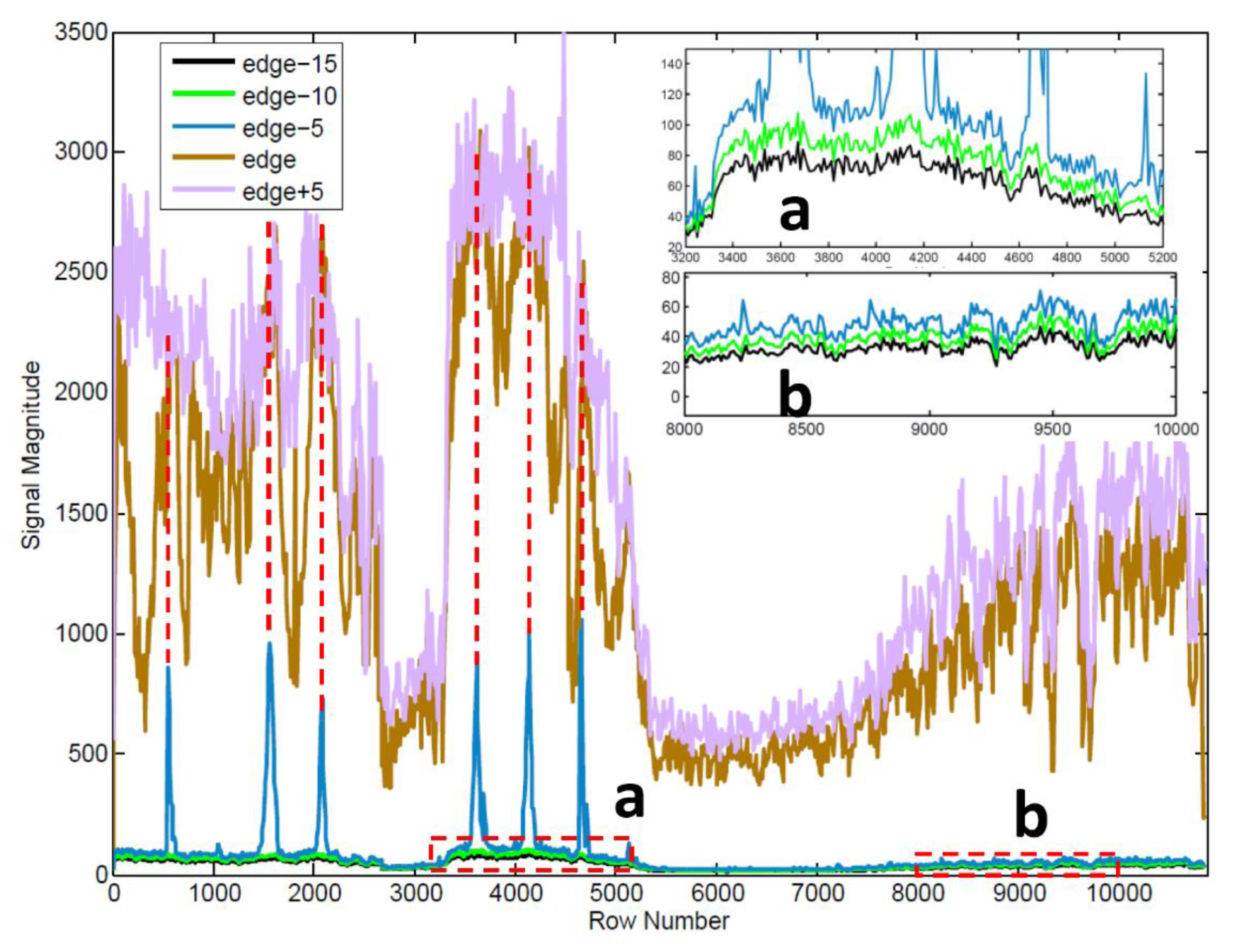
(1) The DN value of the noise is sometimes larger than the low backscattered signals, especially for signals from open sea surface or new sea ice. Because of the observation geometry of SAR, smooth ocean surface or ice surface can reflect transmitted radar waves to a large extent, leading to lower backscatter characteristics in an image. The poor signal close to the BM edge in Figure 8a,b (DN: 84–127) is larger compared with the signal from ocean surface and ice (blue color in Figure 2). Thus, BM elimination by setting a noise threshold could not work. This point found in our study coincides with that from [13].
(2) The noise is not normally or homogeneously distributed along image margins, but directionally varied. As can be seen from Figure 8 and Table 2, the correlation coefficient between ‘edge’ and ‘edge-5’ (‘edge-10’) is all greater than 0.90, and the correlation coefficient between ‘edge’ and ‘edge+5’ is 0.88, from which we can conclude that the signal magnitude of BM edge is highly dependent on the magnitude of the closest effective signals. From the embedded panels (a) and (b) in Figure 8 and Table 3, a stable increase in magnitude can be found from ‘edge-15’ to ‘edge-5’, then to ‘edge’. Large signal magnitudes in ‘edge-5’ usually correspond to strong backscattered surface in ‘edge’, as can be seen from the red dashed line in Figure 8. This phenomenon is not unique to only this image but common for every image. However, in data gaps such as the left side of the blue dashed line in Figure 6c, all signal magnitudes of BM are zero, and this phenomenon does not exist. Thus, we can conclude that the BM close to strong backscattered land surface usually has larger signal magnitude and the signal magnitude of BM usually increases along the BC direction except for data gaps.
(3) The location of effective signal edge is not always the same along direction perpendicular to BC, as can be seen from Figure 6a–c. With fast Fourier transform (FFT) algorithms, signals can be analyzed in the frequency domain, and the signal frequency components can be better found. Here, we consider the magnitude of BM edge as the signal (vertical axis in Figure 9) and row number as the time (horizontal axis in Figure 9). After FFT, the location of BM edge repeated at a cycle of ~516 pixels along image boundaries. Additionally, the location of BM edge varies by 7 or 8 pixels along the BC direction for each edge step (S1–S3 in Figure 6a). Similarly, this cycle can be found from almost every GRD image from Supplementary Figures. For different images, the cycle of BM edge location may differ slightly, ~516 pixels, which may be caused by different observation geometry of Sentinel-1A when operating. Thus, BM elimination by simply giving a specified edge location would cause more effective signal loss or less noise data elimination.
7.3. Parameter Settings
Many parameters used in our method are preset and are critical to the success of BM edge extraction. The threshold of effective signal should differ for different processing units. In this paper, the lowest noise threshold is set as 10 (DN value), but it only works when the noise level is below this value. For the edge detector, the threshold of BM for a searching unit is given as T. Because T is derived from the first image patch fulfilling the normal distribution, the BM threshold does vary for different searching units, which is critical for our edge detector working well over different land surfaces.
Another parameter setting is the size of processed image along four image boundaries. In this paper, we set this as 4000 pixels along the BC direction. Sometimes, the BM edge is far from the image boundary, such as for the right boundary of I-2 from the Supplementary Figures, were a large processing image can ensure the existence of BM edges. However, it does not mean all selected sections of this image will be processed. It is only fully processed when none of the patches along a searching unit fulfill the normal distribution. In this way, the processing time of one image can be shortened.
In the third step of Section 4, 8 of the 10 elements in the same column crossing a threshold are used, and this is a compromise selection for final robust results. Increasing this parameter would lead to more BM. However, decreasing it would result in more effective signals. A threshold of 4 pixels is set when calculating the BM edge jump in Section 4. This is a compromise choice for edge detection. A larger threshold will introduce large uncertainty to BM edge extraction. However, a smaller one would result in fewer accurate edges.
8. Conclusions
The BM of Sentinel-1A GRD images from both EW and IW observation modes is analyzed in this study. The signal magnitude of BM is not always zero and varies from 0 to about 100 (magnitude). The signal magnitude of BM can also be greater than that from low backscattered land surface, such as sea water or glacier slope facing oppositely to the Sentinel-1A. The signal magnitude in BM depends on the closest effective signal to the edge to a large extent, and along the BC direction, the signal magnitude in BM increases if there are no data gaps. Because one GRD image of Sentinel-1A comprises different sub-swath images, the location of the BM edge (the same as edge of effective signals) is not always the same.
An edge detector using normal distribution and the maximum image gradient is designed to detect edges along BC direction. An automatic method to derive BM of Sentinel-1A GRD images was also designed. By comparison with human-interpreted edges, our method was verified to be effective. On average, the error of BM edge extraction with our method is −0.35 ± 0.11 and 0.14 ± 1.38 pixels when considering the perimeter and area difference, respectively. The maximum error of BM edge extraction is about 1.9 ± 3.2 pixel. Our method has the potential to be widely applied and to eliminate the poor data in BM as a first step for further image processing. Since the BM of Sentinel-1A GRD image limits its uses in multidisciplinary applications, we suggest this method be used before mosaicking to study land cover changes of a large area.
Supplementary Materials
The following are available online at https://www.mdpi.com/2072-4292/12/7/1175/s1, Figures S1–S20: Black margin edge extraction results (E0-E9, I0-I9); The MATLAB codes for black margin extraction of Sentinel-1 GRD images can be found in the supplementary materials.
Author Contributions
Conceptualization, X.W.; methodology, X.W.; software, X.W.; validation, X.W., writing—original draft preparation, X.W.; writing—review and editing, D.M.H.; visualization, X.W. All authors have read and agreed to the published version of the manuscript.
Funding
This research was funded by Center for Global Sea Level Change (CSLC) of NYU Abu Dhabi (Grant no: G1204), NSF International Thwaites Glacier Collaboration MELT PLR-1739003, NASA Oceans Melting Greenland (OMG) NNX15AD55G, and NSF Greenland Seal Tagging ARC-1304137.
Acknowledgments
The image data were provided by the European Space Agency.
Conflicts of Interest
The authors declare no conflicts of interest.
References
- Vespe, M.; Greidanus, H. SAR image quality assessment and indicators for vessel and oil spill detection. IEEE Trans. Geosci. Remote Sens. 2012, 50, 4726–4734. [Google Scholar] [CrossRef]
- Chander, G.; Markham, B.L.; Helder, D.L. Summary of current radiometric calibration coefficients for Landsat MSS, TM, ETM+, and EO-1 ALI sensors. Remote Sens. Environ. 2009, 113, 893–903. [Google Scholar] [CrossRef]
- Wang, X.; Cheng, X.; Hui, F.; Cheng, C.; Fok, H.S.; Liu, Y. Xuelong navigation in fast ice near the zhongshan station, antarctica. Mar. Technol. Soc. J. 2014, 48, 84–91. [Google Scholar] [CrossRef]
- Chen, J.; Zhu, X.; Vogelmann, J.E.; Gao, F.; Jin, S. A simple and effective method for filling gaps in Landsat ETM+ SLC-off images. Remote Sens. Environ. 2011, 115, 1053–1064. [Google Scholar] [CrossRef]
- Zhu, X.; Liu, D.; Chen, J. A new geostatistical approach for filling gaps in Landsat ETM+ SLC-off images. Remote Sens. Environ. 2012, 124, 49–60. [Google Scholar] [CrossRef]
- Storey, J.C.; Scaramuzza, P.; Schmidt, G. Landsat 7 scan line corrector-off gap filled product development. In Proceedings of the PECORA 16 Conference Proceedings, Sioux Falls, SD, USA, 23–27 October 2005; pp. 23–27. [Google Scholar]
- Bindschadler, R.; Vornberger, P.; Fleming, A.; Fox, A.; Mullins, J.; Binnie, D.; Paulsen, S.J.; Granneman, D.; Gorodetzky, D. The Landsat image mosaic of Antarctica. Remote Sens. Environ. 2008, 112, 4214–4226. [Google Scholar] [CrossRef]
- Hui, F.; Cheng, X.; Liu, Y.; Zhang, Y.; Ye, Y.; Wang, X.W.; Li, Z.; Wang, K.; Zhan, Z.F.; Guo, J.H.; et al. An improved Landsat image mosaic of Antarctica. Sci. China Earth Sci. 2013, 56, 1–12. [Google Scholar] [CrossRef]
- Brusch, S.; Lehner, S.; Fritz, T.; Soccorsi, M.; Soloviev, A.; Van Schie, B. Ship surveillance with TerraSAR-X. IEEE Trans. Geosci. Remote Sens. 2011, 49, 1092–1103. [Google Scholar] [CrossRef]
- Schwerdt, M.; Schmidt, K.; Ramon, N.; Alfonzo, G.C.; Doring, B.; Zink, M.; Prats, P. Independent verification of the Sentinel-1A system calibration. In Proceedings of the Geoscience and Remote Sensing Symposium (IGARSS), Quebec City, QC, Canada, 3–18 July 2014; pp. 1097–1100. [Google Scholar]
- Schubert, A.; Small, D.; Miranda, N.; Geudtner, D.; Meier, E. Sentinel-1A product geolocation accuracy: Commissioning phase results. Remote Sens. 2015, 7, 9431–9449. [Google Scholar] [CrossRef] [Green Version]
- Schubert, A.; Miranda, N.; Geudtner, D.; Small, D. Sentinel-1A/B combined product geolocation accuracy. Remote Sens. 2017, 9, 607. [Google Scholar] [CrossRef] [Green Version]
- Greidanus, H.; Santamaria, C. First analysis of Sentinel-1 images for maritime surveillance. In Science and Policy Report by the Joint Research Centrel; Publications Office of the European Union: Luxembourg, 2014. [Google Scholar]
- Mouche, A.; Chapron, B. Global C-B and E nvisat, RADARSAT-2 and S entinel-1 SAR measurements in copolarization and cross-polarization. J. Geophys. Res. Ocean. 2015, 120, 7195–7207. [Google Scholar] [CrossRef] [Green Version]
- Available online: http://forum.step.esa.int/t/sar-mosaic/782 (accessed on 1 April 2020).
- Attema, E.; Snoeij, P.; Davidson, M.; Floury, N.; Levrini, G.; Rommen, B.; Rosich, B. The European GMES Sentinel-1 radar mission. In Proceedings of the Geoscience and Remote Sensing Symposium (IGARSS 2008), Boston, MA, USA, 8–11 July 2008; Volume 1, pp. 1–94. [Google Scholar]
- SENTINEL-1 SAR User Guide, ESA. Available online: https://sentinel.esa.int/web/sentinel/user-guides/sentinel-1-sar (accessed on 1 April 2020).
- Torres, R.; Snoeij, P.; Davidson, M.; Bibby, D.; Lokas, S. The Sentinel-1 mission and its application capabilities. In Proceedings of the Geoscience and Remote Sensing Symposium (IGARSS 2012), Munich, Germany, 22–27 July 2012; pp. 1703–1706. [Google Scholar]
- Torres, R.; Snoeij, P.; Geudtner, D.; Bibby, D.; Davidson, M.; Attema, E.; Potin, P.; Rommen, B.; Floury, N.; Brown, M.; et al. GMES Sentinel-1 mission. Remote Sens. Environ. 2012, 120, 9–24. [Google Scholar] [CrossRef]
- Snoeij, P.; Brown, M.; Davidson, M.; Rommen, B.; Floury, N.; Geudtner, D.; Torres, R. Sentinel-1A and Sentinel-1B CSAR status. In Proceedings of the SPIE Remote Sensing, International Society for Optics and Photonics, Prague, Czech Republic, 1 October 2011; p. 817902. [Google Scholar]
- De Zan, F.; Guarnieri, A.M. TOPSAR: Terrain observation by progressive scans. IEEE Trans. Geosci. Remote Sens. 2006, 44, 2352–2360. [Google Scholar] [CrossRef]
- Malenovský, Z.; Rott, H.; Cihlar, J.; Schaepman, M.E.; García-Santos, G.; Fernandes, R.; Berger, M. Sentinels for science: Potential of Sentinel-1,-2, and-3 missions for scientific observations of ocean, cryosphere, and land. Remote Sens. Environ. 2012, 120, 91–101. [Google Scholar] [CrossRef]
- Ardhuin, F.; Collard, F.; Chapron, B.; Girard-Ardhuin, F.; Guitton, G.; Mouche, A.; Stopa, J.E. Estimates of ocean wave heights and attenuation in sea ice using the SAR wave mode on Sentinel-1A. Geophys. Res. Lett. 2015, 42, 2317–2325. [Google Scholar] [CrossRef] [Green Version]
- Guangcai, F.; Zhiwei, L.; Xinjian, S.; Bing, X.; Yanan, D. Source parameters of the 2014 Mw 6.1 South Napa earthquake estimated from the Sentinel 1A, COSMO-SkyMed and GPS data. Tectonophysics 2015, 655, 139–146. [Google Scholar] [CrossRef]
- González, P.J.; Bagnardi, M.; Hooper, A.J.; Larsen, Y.; Marinkovic, P.; Samsonov, S.V.; Wright, T.J. The 2014–2015 eruption of Fogo volcano: Geodetic modeling of Sentinel-1 TOPS interferometry. Geophys. Res. Lett. 2015, 42, 9239–9246. [Google Scholar] [CrossRef] [Green Version]
- Le, T.T.; Atto, A.M.; Trouve, E. Change analysis using multitemporal SENTINEL-1 SAR images. In Proceedings of the Geoscience and Remote Sensing Symposium (IGARSS 2015), Milan, Italy, 26–31 July 2015; pp. 4145–4148. [Google Scholar]
- Lizhen, L.; Tao, Y.; Di, L. Object-based plastic-mulched landcover extraction using integrated Sentinel-1 and Sentinel-2 data. Remote Sens. 2018, 10, 1820. [Google Scholar]
- Muckenhuber, S.; Korosov, A.; Sandven, S. Sea ice drift from Sentinel-1 SAR imagery using open source feature tracking. Cryosphere Discuss. 2015, 9, 6937–6959. [Google Scholar] [CrossRef] [Green Version]
- Pelich, R.; Longepe, N.; Mercier, G.; Hajduch, G.; Garello, R. Performance evaluation of Sentinel-1 data in SAR ship detection. In Proceedings of the Geoscience and Remote Sensing Symposium (IGARSS 2015), Milan, Italy, 26–31 July 2015; pp. 2103–2106. [Google Scholar]
- Velotto, D.; Bentes, C.; Tings, B.; Lehner, S. Comparison of Sentinel-1 and TerraSAR-X for ship detection. In Proceedings of the Geoscience and Remote Sensing Symposium (IGARSS 2015), Milan, Italy, 26–31 July 2015; pp. 3282–3285. [Google Scholar]
- Nagler, T.; Rott, H.; Hetzenecker, M.; Wuite, J.; Potin, P. The Sentinel-1 mission: New opportunities for ice sheet observations. Remote Sens. 2015, 7, 9371–9389. [Google Scholar] [CrossRef] [Green Version]
- Hui, F.; Kang, J.; Liu, Y.; Cheng, X.; Gong, P.; Wang, F.; Li, Z.; Ye, Y.; Guo, Z. AntarcticaLC2000: The new antarctic land cover database for the year 2000. Sci. China Earth Sci. 2017, 60, 686–696. [Google Scholar] [CrossRef]
- Scambos, T.A.; Haran, T.M.; Fahnestock, M.A.; Painter, T.H.; Bohlander, J. MODIS-based mosaic of antarctica (MOA) data sets: Continent-wide surface morphology and snow grain size. Remote Sens. Environ. 2007, 111, 242–257. [Google Scholar] [CrossRef]
- Rignot, E.; Echelmeyer, K.; Krabill, W. Penetration depth of interferometric synthetic-aperture radar signals in snow and ice. Geophys. Res. Lett. 2001, 28, 3501–3504. [Google Scholar] [CrossRef] [Green Version]
- Munk, J.; Jezek, K.C.; Forster, R.R.; Gogineni, S.P. An accumulation map for the Greenland dry-snow facies derived from spaceborne radar. J. Geophys. Res. Atmos. 2003, 108, D9. [Google Scholar] [CrossRef]
- Kendra, J.R.; Sarabandi, K.; Ulaby, F.T. Radar measurements of snow: Experiment and analysis. IEEE Trans. Geosci. Remote Sens. 1998, 36, 864–879. [Google Scholar] [CrossRef] [Green Version]
- Canny, J. A computational approach to edge detection. Pattern Analysis and Machine Intelligence. IEEE Trans. 1986, 6, 679–698. [Google Scholar]
- Ding, L.; Goshtasby, A. On the canny edge detector. Pattern Recognit. 2001, 34, 721–725. [Google Scholar] [CrossRef]
- Roberts, L.G. Machine Perception of Three-Dimensional Soups. Ph.D. Thesis, Massachusetts Institute of Technology, Cambridge, MA, USA, 1963. [Google Scholar]
- Sobel, I.; Feldman, G. A 3 × 3 Isotropic Gradient Operator for Image Processing. Stanf. Artif. Intell. Proj. 1968, 271–272. [Google Scholar]
- Prewitt, J.M. Object enhancement and extraction. Pict. Process. Psychopictorics 1970, 10, 15–19. [Google Scholar]
- David, M.; Hildreth, E. Theory of edge detection. In Proceedings of the Royal Society of London (Series B), London, UK, 29 February 1980; pp. 187–217. [Google Scholar]
- Lilliefors, H.W. On the Kolmogorov-Smirnov test for normality with mean and variance unknown. J. Am. Stat. Assoc. 1967, 62, 399–402. [Google Scholar] [CrossRef]
- Satoshi, T. Completing yearly land cover maps for accurately describing annual changes of tropical landscapes. Glob. Ecol. Conserv. 2018, 13, e00384. [Google Scholar]
Figure 1.
Spatial coverage of Sentinel-1A images from extra wide (EW) and interferometric wide (IW) around Antarctica during May 2015. The total number of images is 899, with 211 of IW images and 688 of EW images. Red and blue rectangles show footprints of EW and IW image respectively. A polar stereographic projection with −71°S as standard latitude is used.
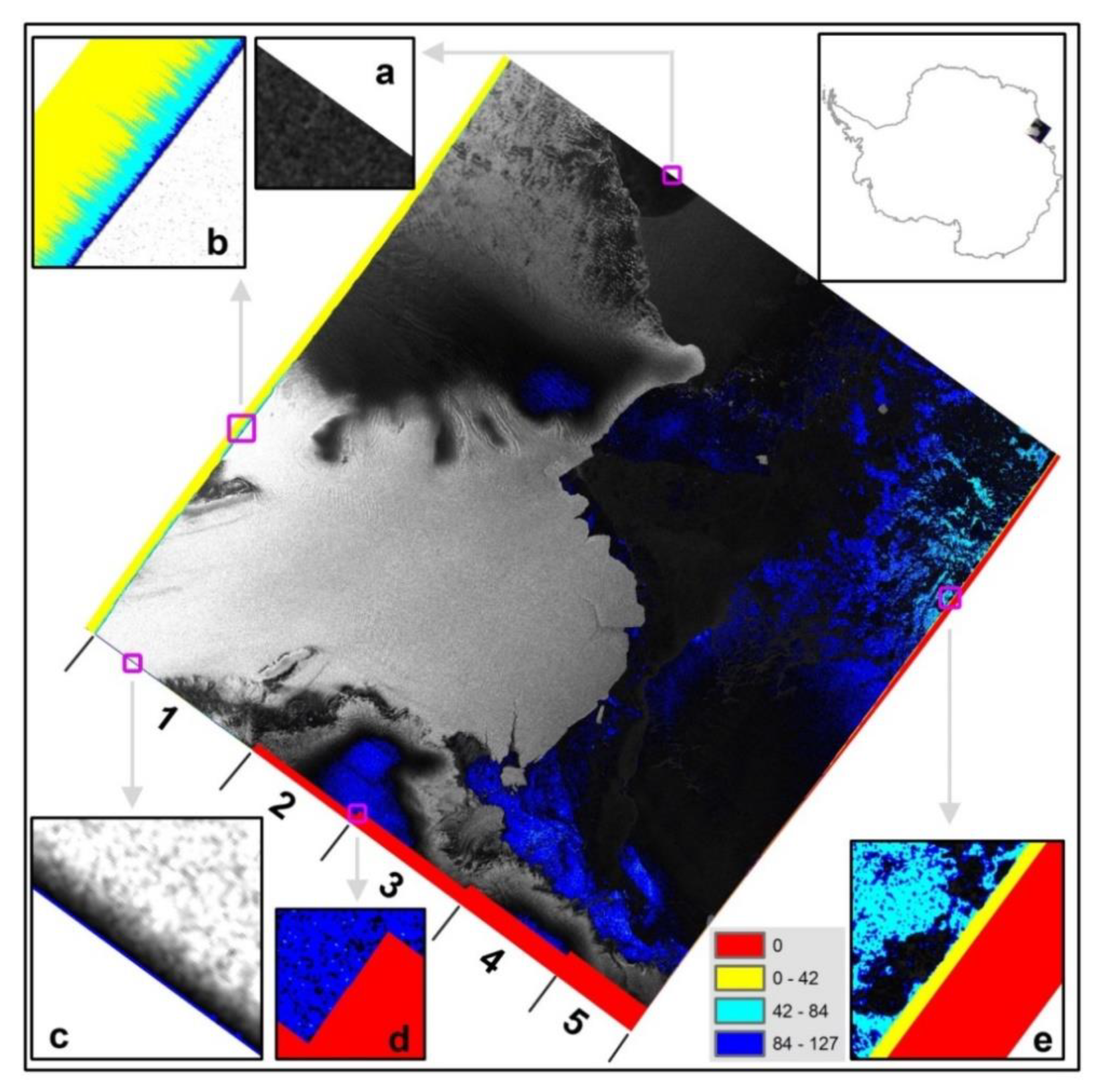
Figure 2.
Poor-quality data around black margins of a Sentinel-1A image (s1a-ew-grd-hh-20151203t152802-20151203t152906-008879-00cb1d-001.tiff). (a) Data cover open sea water, no black margin. (b) Signal backscattered from inland glacier, including black margin (not always zero, as indicated with yellow, green, and cyan, and blue colors) close to the image boundary. (c) Very typical black margins, including poor-quality data with lower signal magnitude increasing from image boundary to image center. (d) Boundary from different sub-swaths with data gap filled with zero. (e) Data over sea water and sea ice, with yellow color indicating poor-quality data. ‘1’ to ‘5’ indicate five sub-swath images used for EW ground range detected (GRD) image mosaic. A polar stereographic projection with −71°S as standard latitude is used.

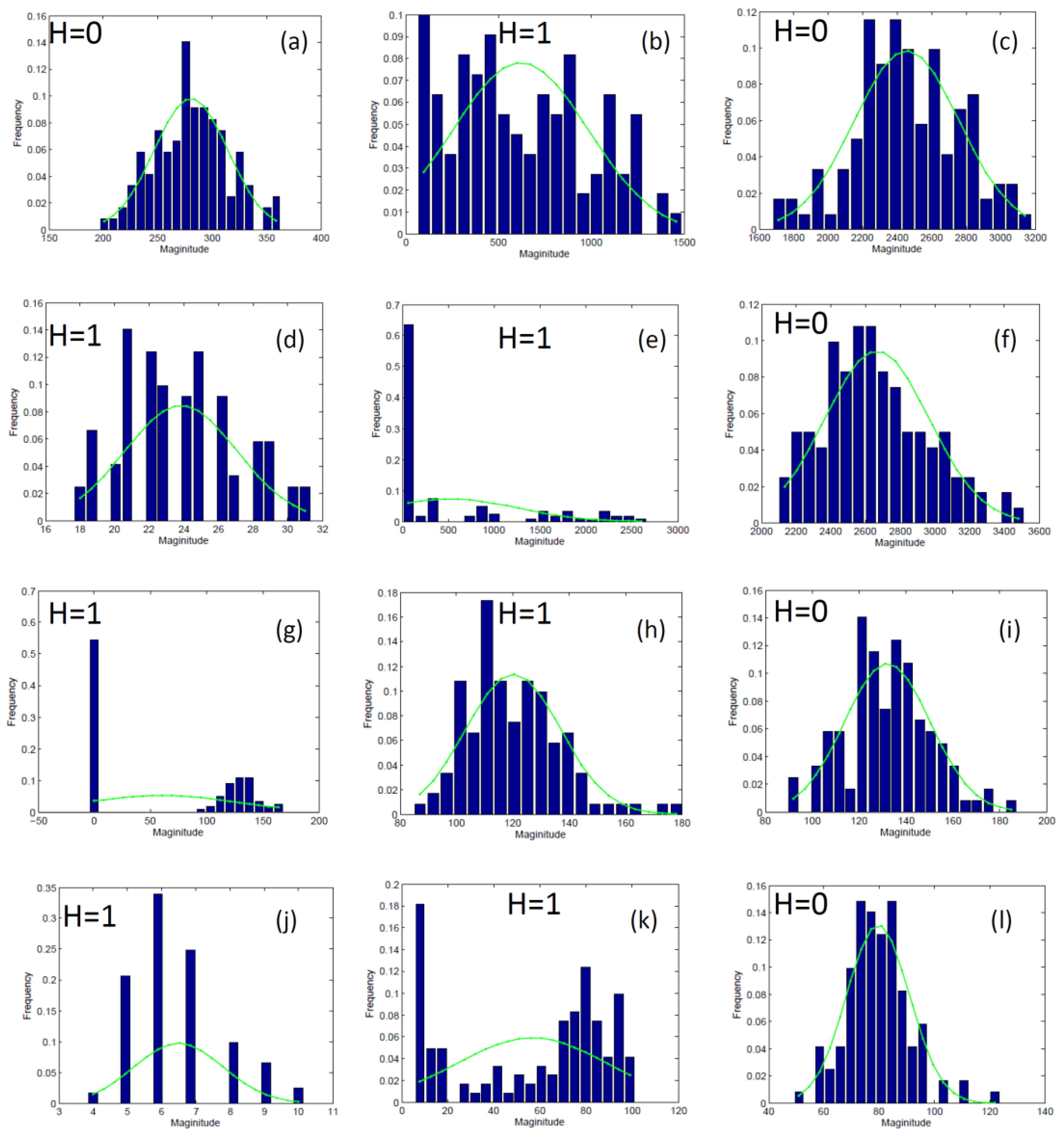
Figure 3.
Signal magnitude histograms of an image patch from different marginal areas. “H = 0” means the data passes the test of normal distribution while “H = 1” means it does not. (a) An image patch with signal magnitude histogram (ocean water) from region A of Figure 2. (b,c) Image patches with magnitude histogram from poor signal (black margin) and effective signal (glacier) respectively in region C of Figure 2. (d–f) Magnitude histograms of image patches from noise, noise + effective signal, and effective signal, respectively, in region B of Figure 2. (g–i) Magnitude histogram changes of signals from data gaps and land surface, non-normally distributed land surface, and normally distributed land surface respectively in region D of Figure 2. (j–l) Magnitude histogram of noise, noise + effective signal, and effective signal, respectively, in region E (sea surface and sea ice region) of Figure 2.

Figure 4.
Sketch plot for edge detection process. This figure shows the process of edge detection from the left boundary of an image. The black dashed rectangle indicates a searching image patch. The green rectangle indicates the first patch fulfilling a normal distribution. The blue line indicates the start location (ET1 in context) where a searching unit firstly crosses a threshold. The block dashed square indicates searching tracks. The purple line indicates the starting location (ET2 in context) for the maximum of gradient change along the column direction. In this figure, the black color shows regions of poor-quality data and the blue color shows effective backscattered signals. ‘1’, ‘2’, ‘m’, ‘n’, and ‘t’ stand for different searching units. A searching unit corresponds to all signals from 10 rows of a processing image. The black margin (BM) edge detection from searching units ‘2’, ‘m’, and ‘n’ is not accepted but is accepted from ‘1’. However, in searching unit ‘t’, no edge is detected.

Figure 5.
Sketch plot for edge detection process. In this figure, ‘BC’ indicates the direction from the image boundary to the image center, the same as what is defined in the context. ‘PBC’ indicates the direction perpendicular to the ‘BC’ direction.
Figure 5.
Sketch plot for edge detection process. In this figure, ‘BC’ indicates the direction from the image boundary to the image center, the same as what is defined in the context. ‘PBC’ indicates the direction perpendicular to the ‘BC’ direction.
Figure 6.
BM edge extraction and results comparison between automatic method and human interpretation. (a–d) correspond to BM edges from the left, right, top, and bottom of (e). Blue dashed squares in (a) indicate different edge steps. ‘S1’, ‘S2’, and ‘S3’ are respectively used for analysis in Figure 9a,c,e. ‘1’ to ‘5’ correspond to BM edges from five sub-swaths as indicated in Figure 2. Vertical dashed blue lines indicate boundaries of data gaps as can be seen from Figure 2. (e) Comparison of BM edge extracted with automatic method (green) and human interpretation (red). Comparison zooming in is marked with ‘A’ to ‘G’. Plotted with image coordinates, thus differing from Figure 2. The image flipping is caused by SAR imaging characteristics.
Figure 7.
Spatial coverage of the sentinel-1A images over Antarctic inland, coast and ocean. ‘E0’ to ‘E9’ are indices for images from the EW observation model. ‘I-0’ to ‘I-9’ stands for images from IW observation mode. A polar stereographic projection with −71°S as standard latitude is used.
Figure 7.
Spatial coverage of the sentinel-1A images over Antarctic inland, coast and ocean. ‘E0’ to ‘E9’ are indices for images from the EW observation model. ‘I-0’ to ‘I-9’ stands for images from IW observation mode. A polar stereographic projection with −71°S as standard latitude is used.

Figure 8.
Signal magnitude (digital number (DN) value) along the BM edge, effective signal region, and black margins in the left side of image shown in Figure 6e. In the legend, ‘edge’ indicates the signal from column corresponding to BM edge. ‘edge+5’ indicates the signal from the fifth column to the right side (signal region) of edge. ‘edge-m’ indicated the signal from the m-th column to the left side (black margin) of edge. Location of the embedded figure (a,b) is marked with a red dashed rectangle using the same marking indices. Vertical dashed red lines indicate the column, which shows good correlation between strong backscattered signals and large noise signals in BM.

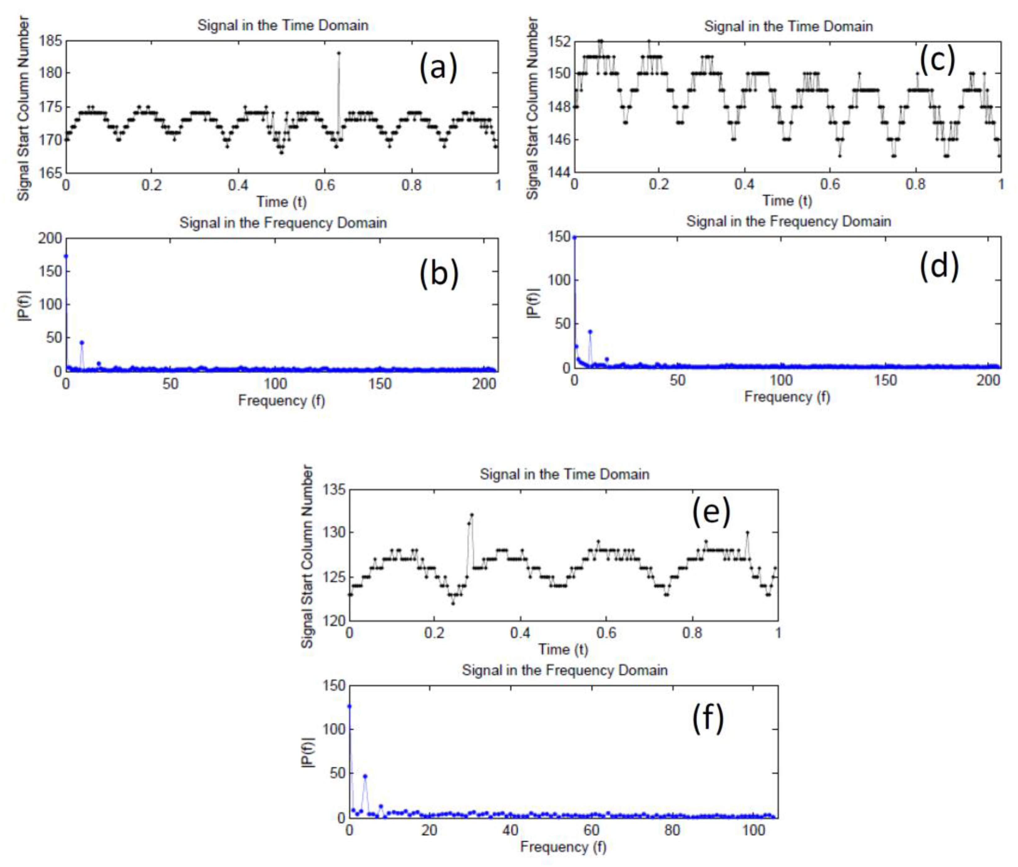
Figure 9.
BM edge location analysis in both time and frequency domains (DN valuse of BM edge and Fast Frequency Transformation resuts). (a,c,e) indicate the DN value of BM edge detected by our automatic method. (b,d,f) are the Fast Frequency Transformation results of data shown in (a,c,e) respectively. From (a,c,e), the cycle of signal start location can be seen clearly and the starting location is not the same as that appears in Figure 8a because it is not smoothed and just a middle output during BM edge detection. In the frequency domains (b,d,f), signal frequencies of 8, 8, and 4 Hz are detected respectively, which indicate the signal cycles in PBC direction are 512, 512, and 525 columns for three different regions.

Table 1.
Validation of the BM edge extracted from our method using human interpretation. ‘Nr’ and ‘Nc’ stand for the number of rows and columns of the image. ‘El’, ‘Er’, ‘Et’, and ‘Eb’ stand for the maximum extraction error of edge on the left, right, top, and bottom. ‘∆P’ and ‘∆A’ respectively stand for differences in perimeter and area of effective signal regions by subtracting automatic derivation results from human interpretation results. All of results are in unit of pixels.
| Observation Mode and Region | Index | File Name | Nr | Ec | El | Er | Et | Eb | ∆P | ∆A | ||
|---|---|---|---|---|---|---|---|---|---|---|---|---|
| EW, coast | E0 | s1a-ew-grd-hh-20150509t011137-20150509t011241-005837-007835-001.tiff | 10,842 | 10,425 | 2 | 7 | 2 | 0 | −239.5 | −96.1 | −0.41 | −0.16 |
| E1 | s1a-ew-grd-hh-20150512t194245-20150512t194350-005892-00796c-001.tiff | 10,844 | 10,524 | 1 | 2 | 5 | 0 | −294.1 | 2681.8 | −0.50 | 4.56 | |
| E2 | s1a-ew-grd-hh-20150514t160932-20150514t161037-005919-007a05-001.tiff | 10,845 | 10,407 | 2 | 4 | 3 | 0 | −331.4 | 957.5 | −0.56 | 1.63 | |
| E3 | s1a-ew-grd-hh-20150523t122738-20150523t122843-006048-007d0d-001.tiff | 10,844 | 10,352 | 2 | 7 | 3 | 0 | −284.4 | 1283.9 | −0.48 | 2.19 | |
| E4 | s1a-ew-grd-hh-20150516t091702-20150516t091802-005944-007a8c-001.tiff | 10,140 | 10,634 | 3 | 3 | 0 | 0 | −214.5 | 59.8 | −0.38 | 0.11 | |
| E5 | s1a-ew-grd-hh-20150507t062249-20150507t062353-005811-007791-001.tiff | 10,844 | 10,556 | 5 | 2 | 8 | 0 | −309.6 | 356.3 | −0.53 | 0.61 | |
| EW, ocean | E6 | s1a-ew-grd-hh-20150508t034807-20150508t034907-005824-0077e4-001.tiff | 10,136 | 10,487 | 1 | 8 | 0 | 0 | −214.5 | 59.8 | −0.38 | 0.11 |
| E7 | s1a-ew-grd-hh-20150505t000443-20150505t000543-005778-0076cb-001.tiff | 10,136 | 10,558 | 2 | 4 | 4 | 0 | −252.6 | −570.4 | −0.44 | −1.00 | |
| E8 | s1a-ew-grd-hh-20150510t213839-20150510t213939-005864-0078c8-001.tiff | 10,136 | 10,630 | 1 | 4 | 0 | 0 | −194.8 | 52.5 | −0.34 | 0.09 | |
| E9 | s1a-ew-grd-hh-20150522t132642-20150522t132742-006034-007ca9-001.tiff | 10,137 | 10,468 | 2 | 3 | 0 | 0 | −211.7 | −64.0 | −0.37 | −0.11 | |
| IW, coast | I-0 | s1a-iw-grd-hh-20150921t144737-20150921t144811-007814-00ae0d-001.tiff | 22,518 | 25,185 | 4 | 22 | 0 | 1 | −405.8 | −3171.3 | −0.31 | −2.40 |
| I-1 | s1a-iw-grd-hh-20150928t175640-20150928t175708-007918-00b0ed-001.tiff | 18,787 | 25,217 | 2 | 3 | 0 | 1 | −355.9 | −490.4 | −0.29 | −0.40 | |
| I-2 | s1a-iw-grd-hh-20150525t034955-20150525t035020-006072-007dbb-001.tiff | 16,900 | 25,413 | 3 | 4 | 0 | 0 | −328.6 | −704.9 | −0.30 | −0.64 | |
| I-3 | s1a-iw-grd-hh-20150531t093429-20150531t093454-006163-008043-001.tiff | 16,900 | 25,164 | 3 | 3 | 0 | 0 | −284.5 | −737.2 | −0.24 | −0.63 | |
| I-4 | s1a-iw-grd-hh-20150523t104902-20150523t104927-006047-007d07-001.tiff | 16,905 | 25,508 | 3 | 3 | 0 | 0 | −320.2 | −248.4 | −0.27 | −0.21 | |
| IW, inland | I-5 | s1a-iw-grd-hh-20150924t213659-20150924t213724-007862-00af6b-001.tiff | 16,907 | 25,504 | 7 | 6 | 0 | 0 | −258.4 | −25.0 | −0.22 | −0.02 |
| I-6 | s1a-iw-grd-hh-20150929t002146-20150929t002211-007922-00b10b-001.tiff | 16,906 | 25,264 | 2 | 3 | 0 | 0 | −273.6 | −309.8 | −0.24 | −0.27 | |
| I-7 | s1a-iw-grd-hh-20150525t021152-20150525t021217-006071-007db4-001.tiff | 16,902 | 25,370 | 4 | 1 | 0 | 0 | −243.6 | −90.7 | −0.21 | −0.08 | |
| I-8 | s1a-iw-grd-hh-20150531t062033-20150531t062058-006161-008036-001.tiff | 16,905 | 25,151 | 3 | 2 | 0 | 0 | −244.4 | −405.4 | −0.21 | −0.35 | |
| I-9 | s1a-iw-grd-hh-20150525t120849-20150525t120914-006077-007de0-001.tiff | 16,906 | 25,638 | 1 | 3 | 0 | 0 | −270.7 | −304.4 | −0.23 | −0.26 |
Table 2.
Correlation coefficients between signals listed in Figure 8.
Table 2.
Correlation coefficients between signals listed in Figure 8.
| Correlation Coefficients | edge+5 | edge | edge-5 | edge-10 | edge-15 |
|---|---|---|---|---|---|
| edge+5 | 1.00 | 0.88 | 0.47 | 0.97 | 0.97 |
| edge | 1.00 | 0.57 | 0.91 | 0.90 | |
| edge-5 | 1.00 | 0.54 | 0.53 | ||
| edge-10 | 1.00 | 0.99 | |||
| edge-15 | 1.00 |
Table 3.
Statistics of signal magnitude difference among signal profiles listed in Figure 8. In this table, ‘XXXX_YYYY’ in the first row indicates difference of DN obtained by subtracting DN of YYYY from DN of XXXX.
Table 3.
Statistics of signal magnitude difference among signal profiles listed in Figure 8. In this table, ‘XXXX_YYYY’ in the first row indicates difference of DN obtained by subtracting DN of YYYY from DN of XXXX.
| edge-10_edge-15 | edge-5_edge-10 | edge_edge-5 | edge+5_edge | |
|---|---|---|---|---|
| min | 2.1 | 3 | 86.5 | -432.3 |
| max | 20.3 | 976.6 | 2783.7 | 2083.5 |
| mean | 8.0 | 33.8 | 1136.6 | 323.6 |
| standard deviation | 4.2 | 108.9 | 597.8 | 349.4 |
© 2020 by the authors. Licensee MDPI, Basel, Switzerland. This article is an open access article distributed under the terms and conditions of the Creative Commons Attribution (CC BY) license (http://creativecommons.org/licenses/by/4.0/).
Share and Cite
MDPI and ACS Style
Wang, X.; Holland, D.M. An Automatic Method for Black Margin Elimination of Sentinel-1A Images over Antarctica. Remote Sens. 2020, 12, 1175. https://doi.org/10.3390/rs12071175
AMA Style
Wang X, Holland DM. An Automatic Method for Black Margin Elimination of Sentinel-1A Images over Antarctica. Remote Sensing. 2020; 12(7):1175. https://doi.org/10.3390/rs12071175
Chicago/Turabian StyleWang, Xianwei, and David M. Holland. 2020. "An Automatic Method for Black Margin Elimination of Sentinel-1A Images over Antarctica" Remote Sensing 12, no. 7: 1175. https://doi.org/10.3390/rs12071175
Note that from the first issue of 2016, this journal uses article numbers instead of page numbers. See further details here.