Integrity Monitoring for Horizontal RTK Positioning: New Weighting Model and Overbounding CDF in Open-Sky and Suburban Scenarios


Abstract
1. Introduction
2. Signal Analysis
2.1. Elevation, C/ and Biases
2.2. The Weighting Function
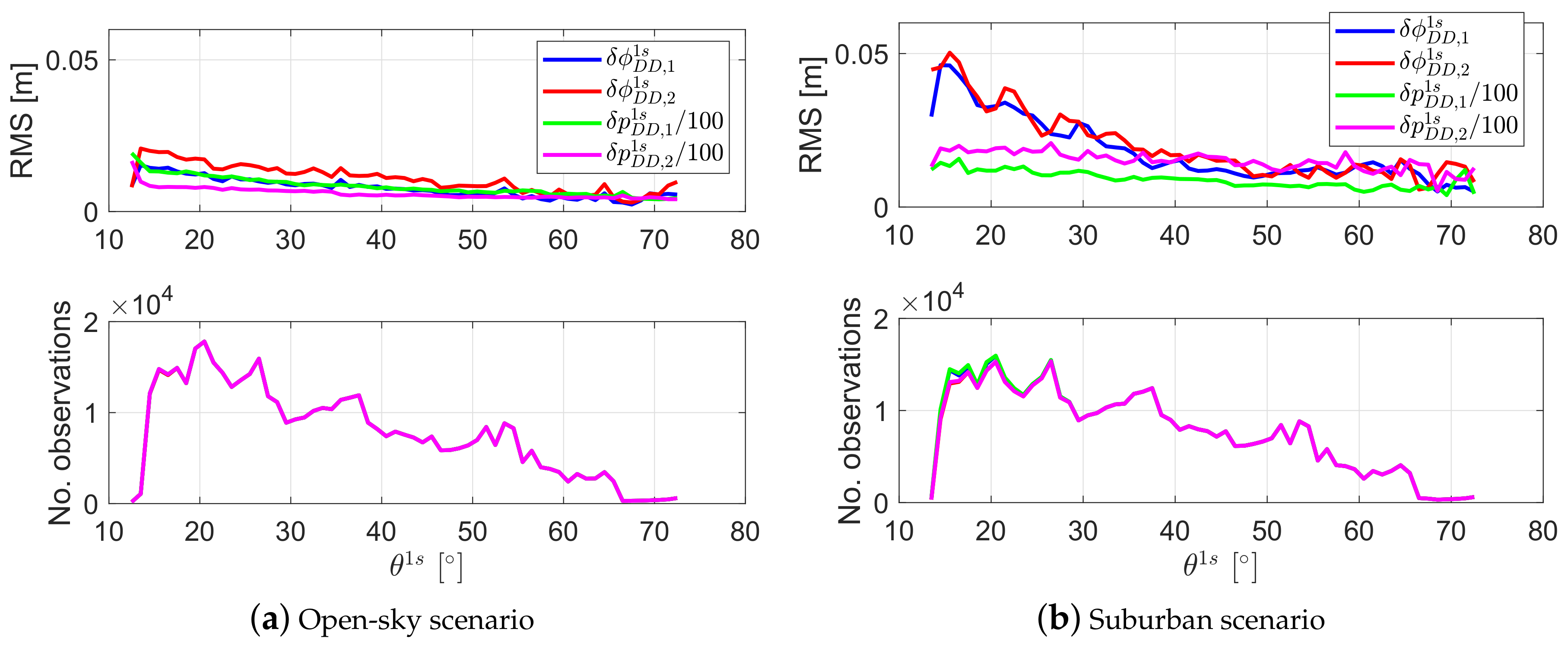
- When and (j=1, 2) are set to zero, i.e., using only the elevation-dependent weighting function in the model.
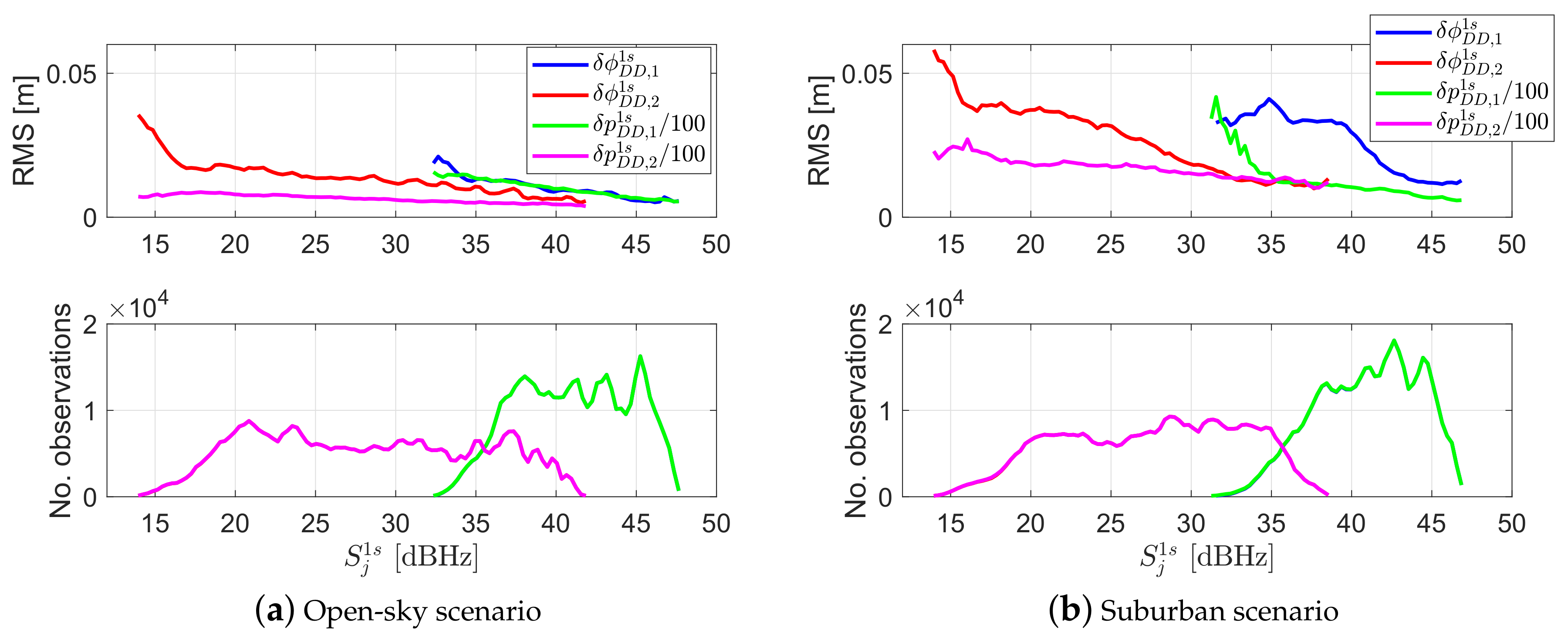
- When and are set to zero, i.e., using only the C/-dependent weighting function in the model.
3. Positioning Method
4. Integrity Monitoring
4.1. Overbounding CDF
4.2. FDE Procedure
4.3. Protection Level
5. Test Results
6. Conclusions
Author Contributions
Funding
Acknowledgments
Conflicts of Interest
Appendix A. Baseline-Known Ambiguity Resolution and the Sequential Exclusion Algorithm
- The number of the excluded phase observations increases from 1 to , where is set to 6 in this contribution.
- For the same number of excluded observations, the observations with low elevation angles have priority in exclusion.
- For the observations with the same elevation angle, the observation on L2 has the priority in exclusion, as in this contribution the observations on L1 are considered as the basis observations to compute, e.g., the position dilution of precision (PDOP). This can be changed to other frequencies depending on the needs of the users.
- In case that exclusion of all the combinations in mentioned above fail the ratio test, the phase observation with the highest exclusion priority is excluded to re-compute the . The exclusion begins then from the beginning.
Appendix B. Sequential Exclusion Algorithm in Baseline-Unknown Case
- The number of the excluded observations increases from 1 to .
- For the same number of excluded observations, code observations have the priority in exclusion.
- For the same observation type (code or phase), the observations with the lowest elevation angle have priority in exclusion.
- For the observations with the same elevation angle, the observation on L2 has the priority in exclusion.
- In case that exclusion of all the combinations in mentioned above fail the ratio test, the observation with the highest exclusion priority is excluded to re-compute the subset (). The exclusion restarts then from the beginning.
References
- Leandro, R.; Landau, H.; Nitschke, M.; Glocker, M.; Seeger, S.; Chen, X.; Deking, A.; BenTahar, M.; Zhang, F.; Ferguson, K.; et al. RTX Positioning: The next generation of cm-accurate real-time GNSS positioning. In Proceedings of the 24th International Technical Meeting of the Satellite Division of the Institute of Navigation (ION GNSS 2011), Portland, OR, USA, 20–23 September 2011; pp. 1460–1475. [Google Scholar]
- Banville, S.; Collins, P.; Zhang, W.; Langley, R.B. Global and regional ionospheric corrections for faster PPP convergence. Navig. J. Inst. Navig. 2014, 61, 115–124. [Google Scholar] [CrossRef]
- Yu, X.; Gao, J. Kinematic precise point positioning using multi-constellation global navigation satellite system (GNSS) observations. ISPRS Int. J. Geo-Inf. 2017, 6, 6. [Google Scholar] [CrossRef]
- Euler, H.J.; Goad, C.C. On optimal filtering of GPS dual frequency observations without using orbit information. Bull. Geod. 1991, 65, 130–143. [Google Scholar] [CrossRef]
- Hartinger, H.; Brunner, F.K. Variances of GPS phase observations: The SIGMA-ϵ model. GPS Solut. 1999, 2, 35–43. [Google Scholar] [CrossRef]
- Wieser, A.; Brunner, F.K. An extended weight model for GPS phase observations. Earth Planets Space 2000, 52, 777–782. [Google Scholar] [CrossRef]
- Kuusniemi, H.; Wieser, A.; Lachapelle, G.; Takala, J. User-level reliability monitoring in urban personal satellite-navigation. IEEE Trans. Aerosp. Electron. Syst. 2007, 43, 1305–1318. [Google Scholar] [CrossRef]
- Tay, S.; Marais, J. Weighting models for GPS pseudorange observations for land transportation in urban canyons. In Proceedings of the 6th European Workshop on GNSS Signals and Signal Processing, Munich, Germany, 2–5 December 2013; HAL ID hal-00942180. p. 4. [Google Scholar]
- Medina, D.; Gibson, K.; Ziebold, R.; Closas, P. Determination of pseudorange error models and multipath characterization under signal-degraded scenarios. In Proceedings of the ION GNSS+ 2018, Miami, FL, USA, 24–28 September 2018; pp. 3446–3456. [Google Scholar]
- Wang, J.; Stewart, M.P.; Tsakiri, M. Stochastic modeling for static GPS baseline data processing. J. Surv. Eng. 1998, 124, 171–181. [Google Scholar] [CrossRef]
- Wang, J. Stochastic modeling for real-time kinematic GPS/glonass positioning. Navig. J. Inst. Navig. 1999, 46, 297–305. [Google Scholar] [CrossRef]
- Wang, J.; Satirapod, C.; Rizos, C. Stochastic assessment of GPS carrier phase measurements for precise static relative positioning. J. Geod. 2002, 76, 95–104. [Google Scholar] [CrossRef]
- Blanch, J.; Walter, T.; Enge, P.; Lee, Y.; Pervan, B.; Rippl, M.; Spletter, A. Advanced RAIM user algorithm description: Integrity support message processing, fault detection, exclusion, and protection level calculation. In Proceedings of the ION GNSS 2012, Nashville, TN, USA, 17–21 September 2012; pp. 2828–2849. [Google Scholar]
- ARAIM Technical Subgroup. EU-U.S. Cooperation on Satellite Navigation, Working Group C—ARAIM Technical Subgroup, Milestone 3 Report, Final Version; 25 February 2016. Available online: https://ec.europa.eu/growth/content/release-eu-us-cooperation-satellite-navigation-working-group-c-araim-technical-subgroup-0_en (accessed on 4 April 2020).
- Jiang, Y.; Wang, J. A New Approach to Calculate the Horizontal Protection Level. J. Navig. 2016, 69, 57–74. [Google Scholar] [CrossRef]
- El-Mowafy, A.; Kubo, N. Integrity monitoring of vehicle positioning in urban environment using RTK-GNSS, IMU and speedometer. Meas. Sci. Technol. 2017, 28, 055102. [Google Scholar] [CrossRef]
- El-Mowafy, A.; Imparato, D.; Rizos, C.; Wang, J.; Wang, K. On hypothesis testing in RAIM algorithms: Generalized likelihood ratio test, solution separation test and a possible alternative. Meas. Sci. Technol. 2019, 2019 30, 075001. [Google Scholar] [CrossRef]
- Blanch, J.; Walter, T.; Enge, P. Optimal positioning for advanced Raim. Navig. J. Inst. Navig. 2013, 60, 279–289. [Google Scholar] [CrossRef]
- Gunning, K.; Blanch, J.; Walter, T.; De Groot, L.; Norman, L. Design and evaluation of integrity algorithms for PPP in kinematic applications. In Proceedings of the ION GNSS+ 2018, Miami, FL, USA, 24–28 September 2018; pp. 1910–1939. [Google Scholar]
- El-Mowafy, A.; Kubo, N. Integrity monitoring for positioning of intelligent transport systems using integrated RTK-GNSS, IMU and vehicle odometer. IET Intell. Transp. Syst. 2018, 12, 901–908. [Google Scholar] [CrossRef]
- Imparato, D.; El-Mowafy, A.; Rizos, C.; Wang, J. Vulnerabilities in SBAS and RTK Positioning in Intelligent Transport Systems: An Overview. In Proceedings of the IGNSS Symposium 2018, Colombo Theatres, Kensington Campus, UNSW, Sydney, NSW, Australia, 7–9 February 2018. [Google Scholar]
- Yasyukevich, Y.; Astafyeva, E.; Padokhin, A.; Ivanova, V.; Syrovatskii, S.; Podlesnyi, A. The 6 September 2017 X-class solar flares and their impacts on the ionosphere, GNSS, and HF radio wave propagation. Space Weather 2018, 16, 1013–1027. [Google Scholar] [CrossRef] [PubMed]
- Blagoveshchensky, D.V.; Sergeeva, M.A. Impact of geomagnetic storm of September 7–8, 2017 on ionosphere and HF propagation: A multi-instrument study. Adv. Space Res. 2019, 63, 239–256. [Google Scholar] [CrossRef]
- Demyanov, V.V.; Zhang, X.; Lu, X. Moderate geomagnetic storm condition, WAAS Alerts and real GPS positioning quality. J. Atmos. Sci. Res. 2019, 2, 10–23. [Google Scholar] [CrossRef]
- Teunissen, P.J.G.; Montenbruck, O. Springer Handbook of Global Navigation Satellite Systems; Springer International Publishing: Cham, Switzerland, 2017. [Google Scholar]
- Saastamoinen, J. Contribution to the theory of atmospheric refraction. Bull. Geod. 1972, 105, 279–298. [Google Scholar] [CrossRef]
- Ifadis, I.I. The Atmospheric Delay of Radio Waves: Modelling the Elevation Dependence on a Global Scale; Technical Report No 38L; Chalmers University of Technology: Gothenburg, Sweden, 1986. [Google Scholar]
- Zaminpardaz, S.; Wang, K.; Teunissen, P.J.G. Australia-first high-precision positioning results with new Japanese QZSS regional satellite system. GPS Solut. 2018, 22, 101. [Google Scholar] [CrossRef]
- Teunissen, P.J.G. Least-Squares Estimation of the Integer GPS Ambiguities; Technical report, LGR Series, No.6; Delft Geodetic Computing Centre: Delft, The Netherlands, 1993; pp. 59–74. [Google Scholar]
- Teunissen, P.J.G. The least-squares ambiguity decorrelation adjustment: A method for fast GPS ambiguity estimation. J. Geod. 1995, 70, 65–82. [Google Scholar] [CrossRef]
- Chang, X.W.; Yang, X.; Zhou, T. MLAMBDA: A modified LAMBDA method for integer least-squares estimation. J. Geod. 2005, 79, 552–565. [Google Scholar] [CrossRef]
- Teunissen, P.J.G.; Verhagen, S. On the foundation of the popular ratio test for GNSS ambiguity resolution. In Proceedings of the ION GNSS 2004, Long Beach, CA, USA, 21–24 September 2004; pp. 2529–2540. [Google Scholar]
- Leick, A. GPS Satellite Surveying, 3rd ed.; John Wiley and Sons: New York, NY, USA, 2004. [Google Scholar]
- ABM and IPS. GPS Driven Total Electron Content (TEC) Map for the Australian Region. Australian Bureau of Meteorology/Space Weather Branch (IPS). Available online: ftp://ftp-out.sws.bom.gov.au/wdc/gnss/data/tecmaps/ (accessed on 18 October 2019).
- ABM. Daily Rainfall Data. Australian Bureau of Meteorology. Available online: http://www.bom.gov.au/climate/data/ (accessed on 18 October 2019).
- RINEX 3.03. RINEX, The Receiver Independent Exchange Format, Version 3.03; International GNSS Service (IGS), RINEX Working Group and Radio Technical Commission for Maritime Services Special Committee 104 (RTCM-SC104); 14 July 2015. Available online: https://kb.igs.org/hc/en-us/articles/206482558-RINEX-3-03-Release-Notes (accessed on 4 April 2020).
- Zhou, W.; Liu, L.; Huang, L.; Yao, Y.; Chen, J.; Li, S. A new GPS SNR-Based Combination Approach for Land Surface Snow Depth Monitoring. Sci. Rep. 2019, 9, 3814. [Google Scholar] [CrossRef] [PubMed]
- Amiri-Simkooei, A.R.; Teunissen, P.J.G.; Tiberius, C.C.J.M. Application of least-squares variance component estimation to GPS observables. J. Surv. Eng. 2009, 135, 149–160. [Google Scholar] [CrossRef]
- Verhagen, S.; Teunissen, P.J.G. Least-Squares Estimation and Kalman Filtering. In Springer Handbook of Global Navigation Satellite Systems; Teunissen, P.J.G., Montenbruck, O., Eds.; Springer International Publishing: Cham, Switzerland, 2017; pp. 639–660. [Google Scholar]
- Teunissen, P.J.G.; Joosten, P.; Tiberius, C.C.J.M. Geometry-free ambiguity success rates in case of partial fixing. In Proceedings of the NTM ION 1999, San Diego, CA, USA, 25–27 January 1999; pp. 201–207. [Google Scholar]
- Nardo, A.; Li, B.; Teunissen, P.J.G. Partial ambiguity resolution for ground and space-based applications in a GPS + Galileo scenario: A simulation study. Adv. Space Res. 2016, 57, 30–45. [Google Scholar] [CrossRef]
- GEAS. Phase II of the GNSS Evolutionary Architecture Study. February 2010. Available online: https://www.faa.gov/about/office_org/headquarters_offices/ato/service_units/techops/navservices/gnss/library/documents/media/geasphaseii_final.pdf (accessed on 4 April 2020).
- El-Mowafy, A.; Yang, C. Limited sensitivity analysis of ARAIM availability for LPV-200 over Australia using real data. Adv. Space Res. 2016, 57, 659–670. [Google Scholar] [CrossRef]
- Rife, J.; Walter, T.; Blanch, J. Overbounding SBAS and GBAS error distributions with excess-mass functions. In Proceedings of the 2004 International Symposium on GNSS/GPS, Sydney, Australia, 6–8 December 2004. [Google Scholar]
- Rife, J.; Pullen, S.; Enge, P.; Pervan, B. Paired overbounding for nonideal LAAS and WAAS error distributions. IEEE Trans. Aerop. Electron. Syst. 2006, 42, 1386–1395. [Google Scholar] [CrossRef]
- El-Mowafy, A. On detection of observation faults in the observation and position domains for positioning of intelligent transport systems. J. Geod. 2019, 93, 2109–2122. [Google Scholar] [CrossRef]
- El-Rabbany, A. Introduction to GPS: The Global Positioning System; Artech House: Norwood, MA, USA, 2002. [Google Scholar]
- Teunissen, P.J.G.; De Bakker, P.F. Next generation GNSS single receiver cycle slip reliability. In VII Hotine-Marussi Symposium on Mathematical Geodesy; Sneeuw, N., Novák, P., Crespi, M., Sansò, F., Eds.; International Association of Geodesy Symposia; Springer: Berlin/Heidelberg, Germany, 2012; Volume 137, pp. 159–164. [Google Scholar]


| Receiver | Function | Receiver Type | Antenna Type |
|---|---|---|---|
| UWA0 | Reference receiver | SEPT POLARX5 | JAVRINGANT_DM SCIS |
| CUT0 | Rover (Open-sky scenario) | TRIMBLE NetR9 | TRM59800.00 SCIS |
| SUB0 | Rover (Suburban scenario) | TRIMBLE R10 | TRMR10 NONE |
| Scenario | Phase | Code | ||||||||
|---|---|---|---|---|---|---|---|---|---|---|
| [Hz] | [Hz] | [m] | [Hz] | [Hz] | [m] | |||||
| Open-sky scenario | 10 | 0 | 16.40% | 0.003 | 2 | 0 | 12.67% | 0.096 | ||
| Suburban scenario | 16 | 4000 | 34.11% | 0.018 | 0 | 7000 | 18.81% | 0.255 | ||
| = 0 | = 0 | |||||||||
| Open-sky scenario | 16 | – | – | 8.44% | 0.001 | 6 | – | – | 7.55% | 0.057 |
| Suburban scenario | 16 | – | – | 24.60% | 0.013 | 4 | – | – | 8.41% | 0.114 |
| = 0 | = 0 | |||||||||
| Open-sky scenario | – | 13.50% | 0.002 | – | 0 | 9.96% | 0.076 | |||
| Suburban scenario | – | 4000 | 7.30% | 0.004 | – | 7000 | 18.81% | 0.255 | ||
| Scenario | [m] | [m] | [m] | [m] |
|---|---|---|---|---|
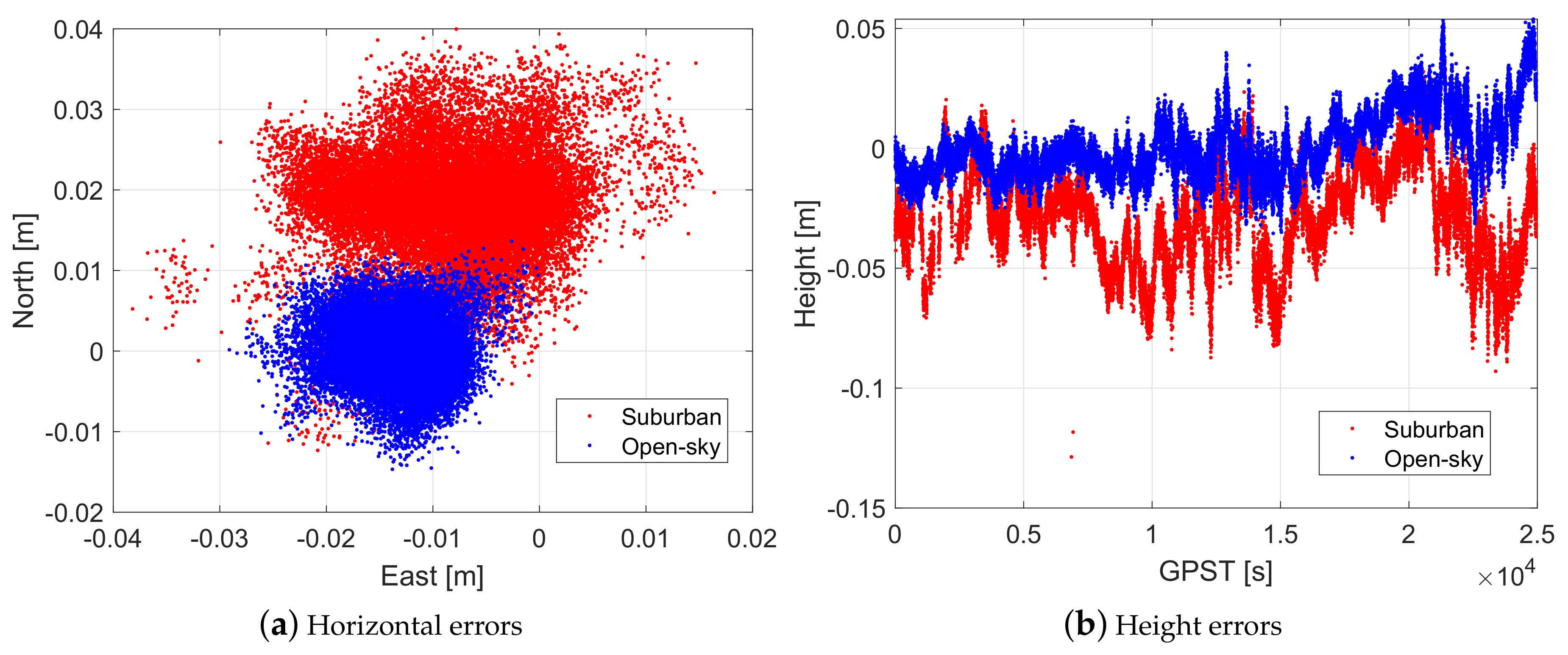
| Open-sky scenario | 0.004 | 0.003 | 0.462 | 0.399 |
| Suburban scenario | 0.007 | 0.005 | 0.555 | 0.490 |
| Scenario | L1 Phase [m] | L2 Phase [m] | C1 Code [m] | C2 Code [m] | ||||
|---|---|---|---|---|---|---|---|---|
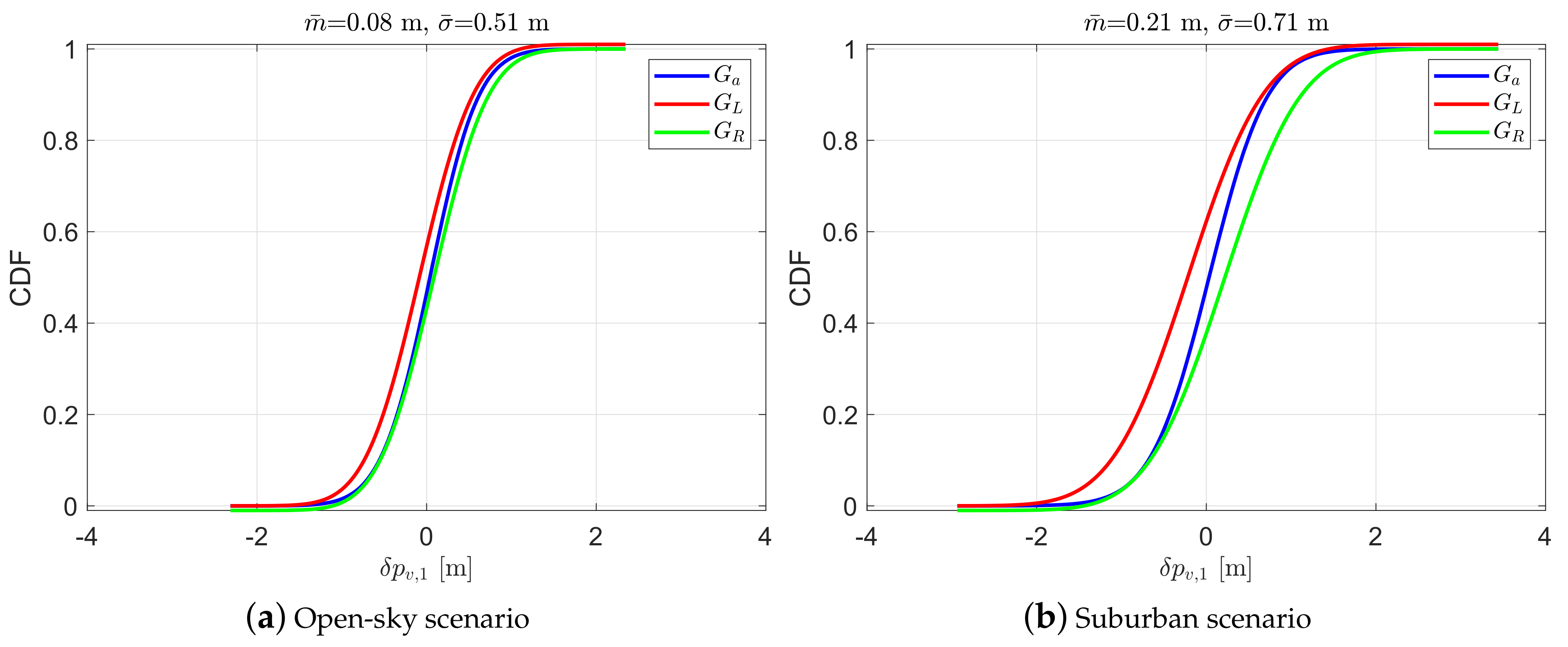
| Open-sky scenario | 0.003 | 0.004 | 0.003 | 0.003 | 0.08 | 0.51 | 0.11 | 0.49 |
| Suburban scenario | 0.002 | 0.006 | 0.003 | 0.006 | 0.21 | 0.71 | 0.23 | 0.59 |
| Scenario | RMS of Fixed HPEs | Mean HPLs | Epochs with FAR | Mean Fix-Rate for PAR | Availability |
|---|---|---|---|---|---|
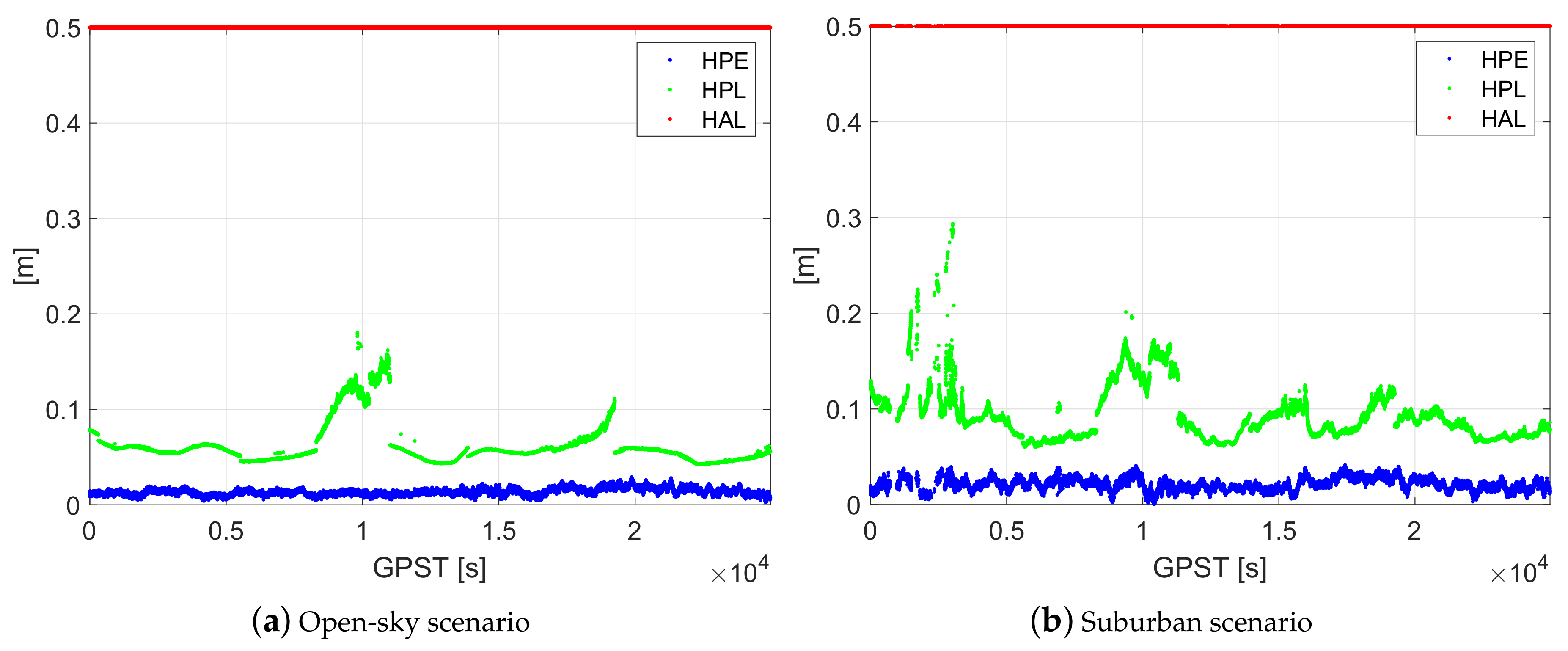
| Open-sky scenario | 0.014/0.009 | 0.062/0.060 | 99.98%/100% | 92.8%/– | 100%/100% |
| Suburban scenario | 0.022/0.017 | 0.093/0.088 | 94.50%/99.96% | 90.6%/91.0% | 100%/100% |
© 2020 by the authors. Licensee MDPI, Basel, Switzerland. This article is an open access article distributed under the terms and conditions of the Creative Commons Attribution (CC BY) license (http://creativecommons.org/licenses/by/4.0/).
Share and Cite
Wang, K.; El-Mowafy, A.; Rizos, C.; Wang, J. Integrity Monitoring for Horizontal RTK Positioning: New Weighting Model and Overbounding CDF in Open-Sky and Suburban Scenarios. Remote Sens. 2020, 12, 1173. https://doi.org/10.3390/rs12071173
Wang K, El-Mowafy A, Rizos C, Wang J. Integrity Monitoring for Horizontal RTK Positioning: New Weighting Model and Overbounding CDF in Open-Sky and Suburban Scenarios. Remote Sensing. 2020; 12(7):1173. https://doi.org/10.3390/rs12071173
Chicago/Turabian StyleWang, Kan, Ahmed El-Mowafy, Chris Rizos, and Jinling Wang. 2020. "Integrity Monitoring for Horizontal RTK Positioning: New Weighting Model and Overbounding CDF in Open-Sky and Suburban Scenarios" Remote Sensing 12, no. 7: 1173. https://doi.org/10.3390/rs12071173
APA StyleWang, K., El-Mowafy, A., Rizos, C., & Wang, J. (2020). Integrity Monitoring for Horizontal RTK Positioning: New Weighting Model and Overbounding CDF in Open-Sky and Suburban Scenarios. Remote Sensing, 12(7), 1173. https://doi.org/10.3390/rs12071173