The Value of Distributed High-Resolution UAV-Borne Observations of Water Surface Elevation for River Management and Hydrodynamic Modeling

 , ,
, ,
Abstract
1. Introduction
2. Materials and Methods
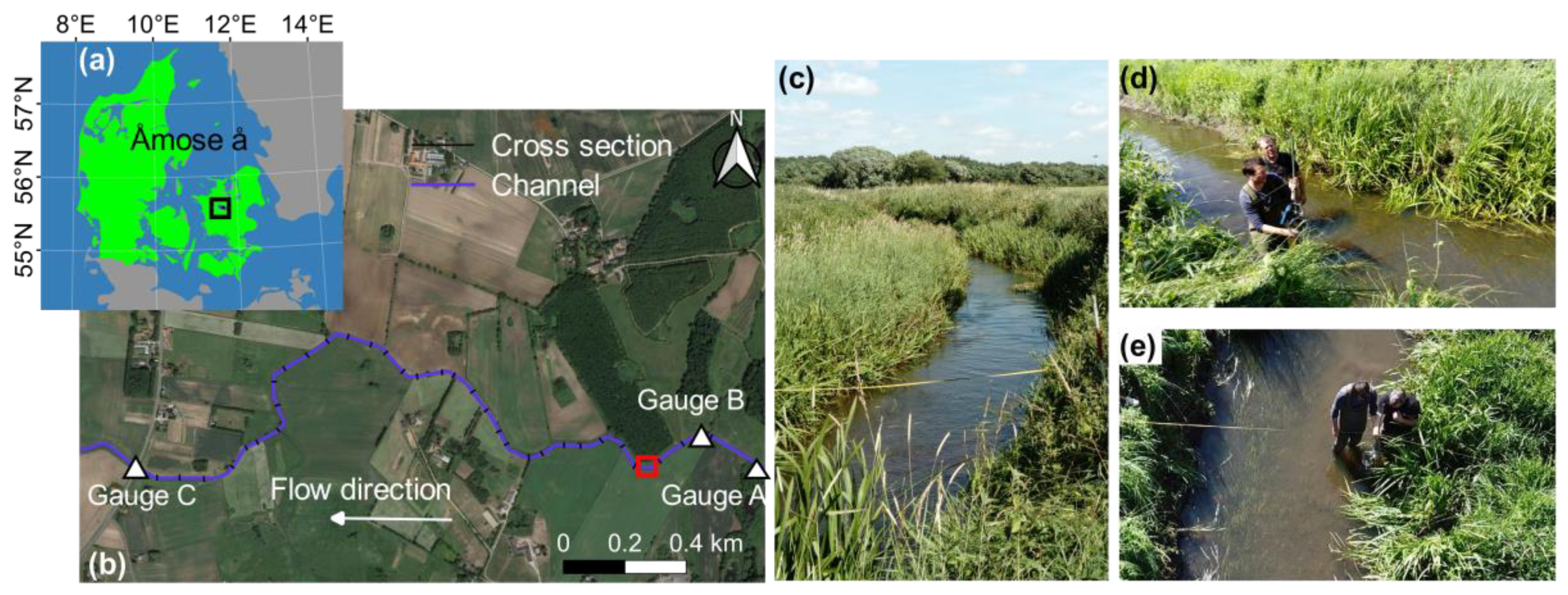
2.1. Study Area
2.2. Data Collection
2.3. Data Processing
2.4. River Model Setup
2.5. Calibration
3. Results
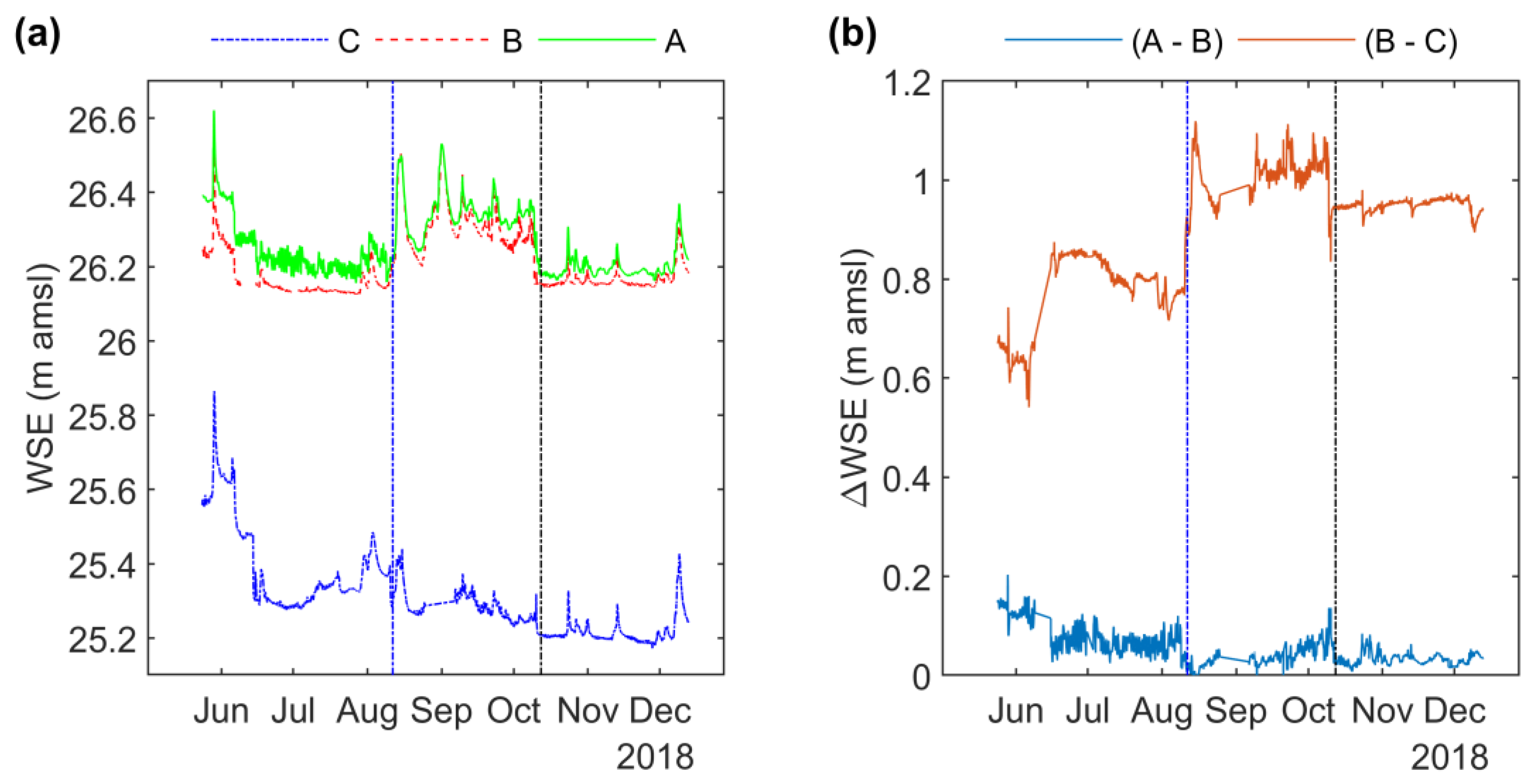
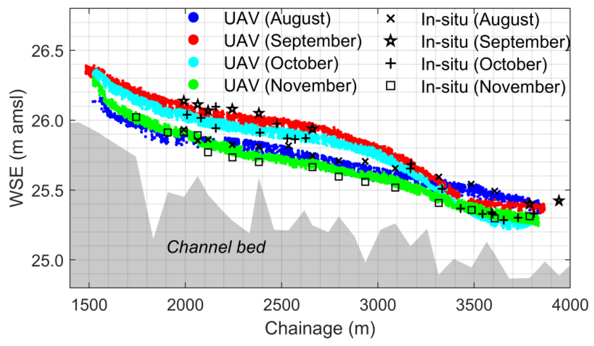
3.1. UAV-Borne WSE
3.2. Calibration of a Hydrodynamic Model
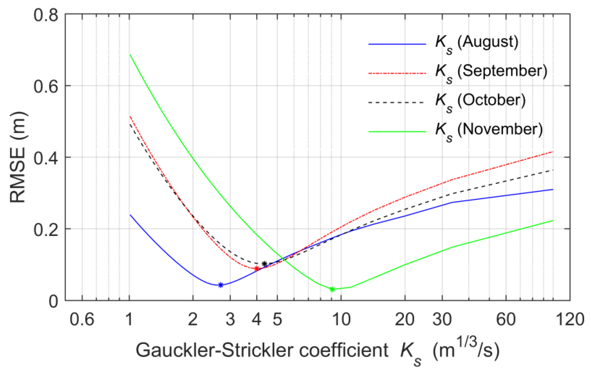
3.2.1. Sensitivity Analysis of Gauckler–Strickler Ks
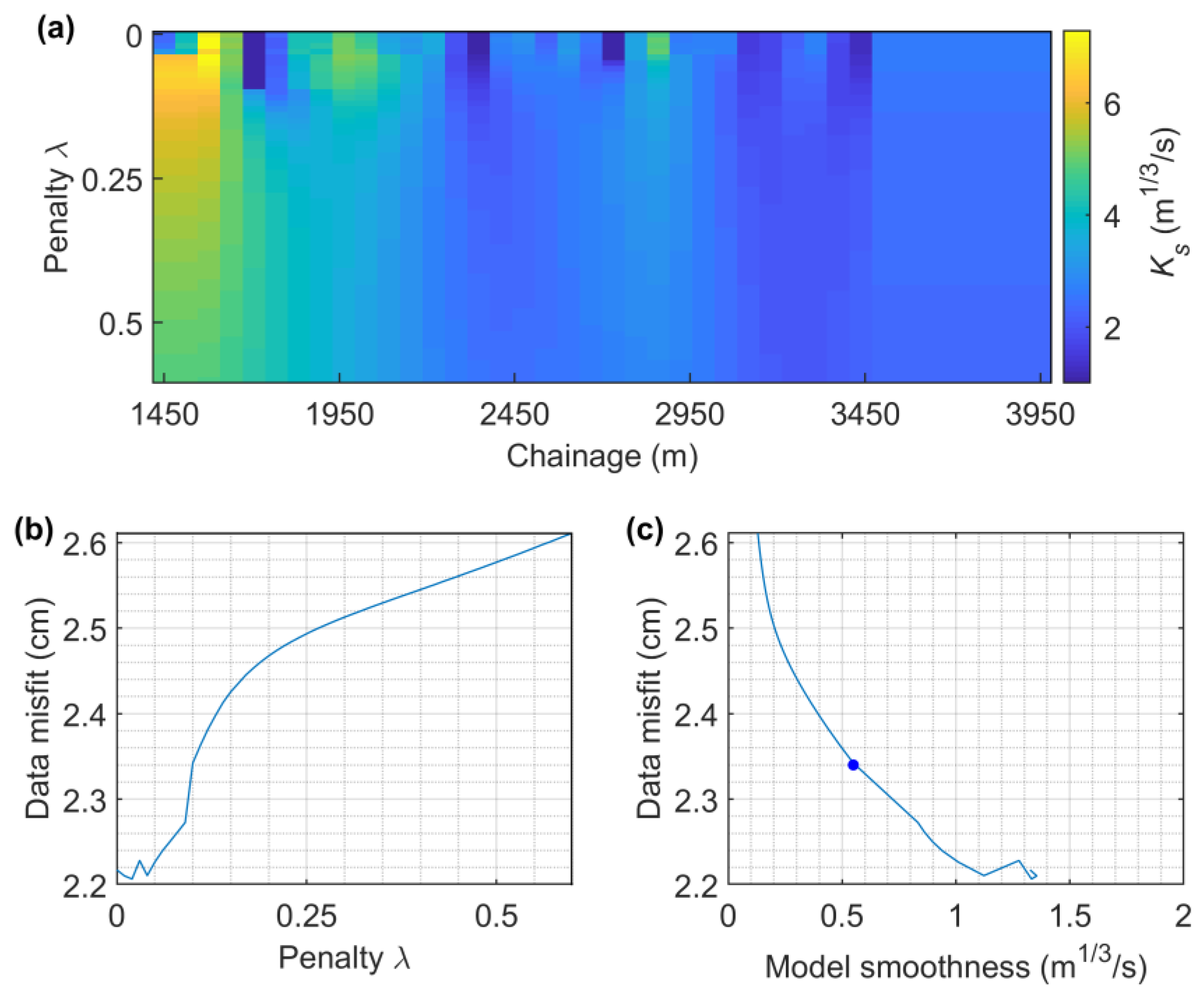
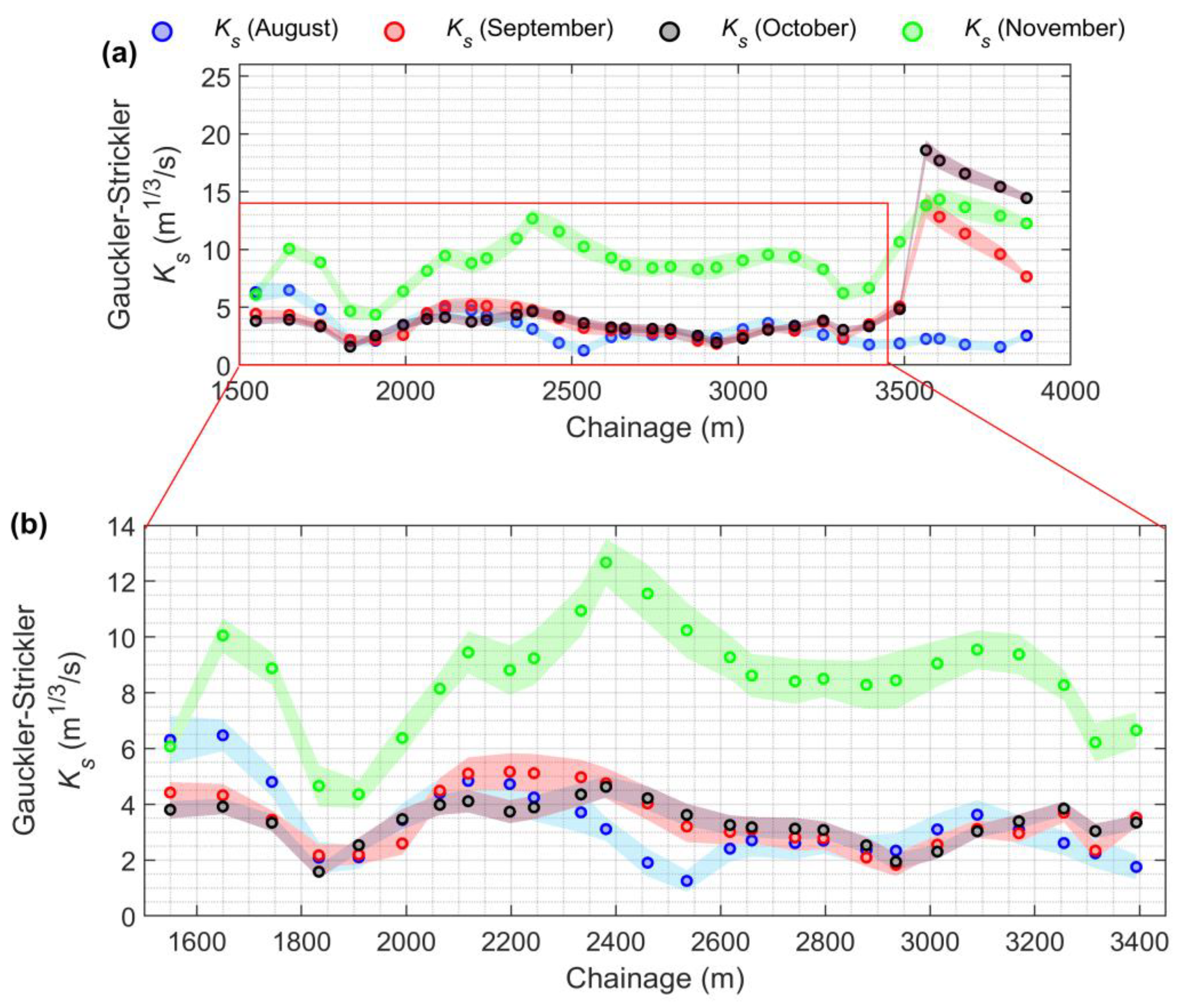
3.2.2. Spatio-Temporal Variation of the Gauckler–Strickler Ks
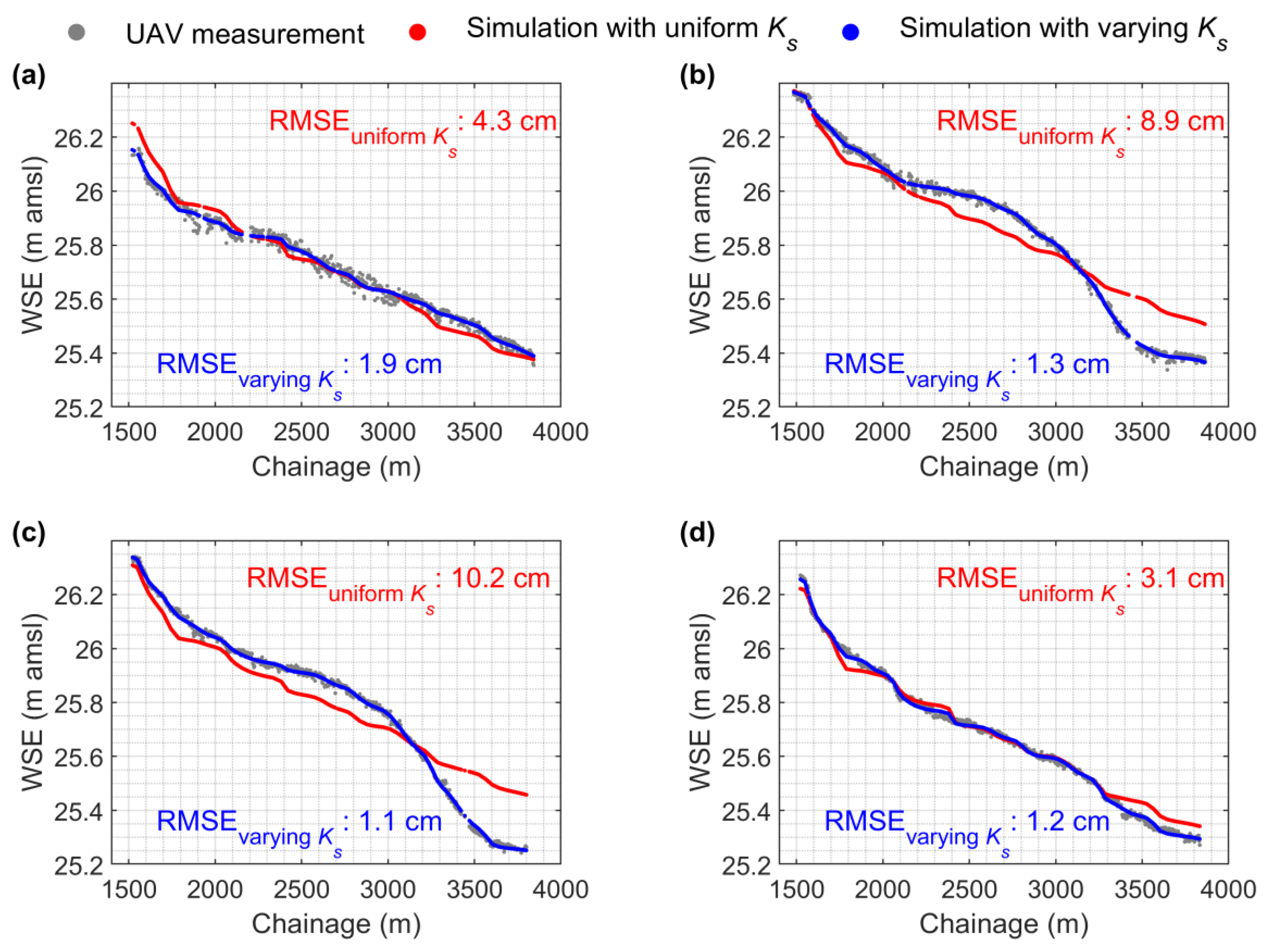
3.2.3. Comparison of Model Performance using Distributed and Uniform Gauckler–Strickler Ks
4. Discussion
5. Summary and Conclusions
Author Contributions
Funding
Conflicts of Interest
References
- Blöschl, G.; Gaál, L.; Hall, J.; Kiss, A.; Komma, J.; Nester, T.; Parajka, J.; Perdigão, R.A.P.; Plavcová, L.; Rogger, M.; et al. Increasing river floods: Fiction or reality? Wiley Interdiscip. Rev. Water 2015, 2, 329–344. [Google Scholar] [CrossRef] [PubMed]
- Tauro, F.; Selker, J.; van de Giesen, N.; Abrate, T.; Uijlenhoet, R.; Porfiri, M.; Manfreda, S.; Caylor, K.; Moramarco, T.; Benveniste, J.; et al. Measurements and Observations in the XXI century (MOXXI): Innovation and multi-disciplinarity to sense the hydrological cycle. Hydrol. Sci. J. 2018, 63, 169–196. [Google Scholar] [CrossRef]
- Bauer-Gottwein, P.; Jensen, I.H.; Guzinski, R.; Bredtoft, G.K.T.; Hansen, S.; Michailovsky, C.I. Operational river discharge forecasting in poorly gauged basins: The Kavango River basin case study. Hydrol. Earth Syst. Sci. 2015, 19, 1469–1485. [Google Scholar] [CrossRef]
- Chang, C.-H.; Lee, H.; Hossain, F.; Basnayake, S.; Jayasinghe, S.; Chishtie, F.; Saah, D.; Yu, H.; Sothea, K.; Du Bui, D. A model-aided satellite-altimetry-based flood forecasting system for the Mekong River. Environ. Model. Softw. 2019, 112, 112–127. [Google Scholar] [CrossRef]
- Crochemore, L.; Ramos, M.H.; Pappenberger, F.; Perrin, C. Seasonal streamflow forecasting by conditioning climatology with precipitation indices. Hydrol. Earth Syst. Sci. 2017, 21, 1573–1591. [Google Scholar] [CrossRef]
- Grimaldi, S.; Li, Y.; Pauwels, V.R.N.; Walker, J.P. Remote Sensing-Derived Water Extent and Level to Constrain Hydraulic Flood Forecasting Models: Opportunities and Challenges. Surv. Geophys. 2016, 37, 977–1034. [Google Scholar] [CrossRef]
- Michailovsky, C.I.; Bauer-Gottwein, P. Operational reservoir inflow forecasting with radar altimetry: The Zambezi case study. Hydrol. Earth Syst. Sci. 2014, 18, 997–1007. [Google Scholar] [CrossRef]
- Neal, J.; Schumann, G.; Bates, P. A subgrid channel model for simulating river hydraulics and floodplain inundation over large and data sparse areas. Water Resour. Res. 2012, 48, 1–16. [Google Scholar] [CrossRef]
- Paiva, R.C.D.; Collischonn, W.; Bonnet, M.-P.; de Gonçalves, L.G.G.; Calmant, S.; Getirana, A.; Santos da Silva, J. Assimilating in situ and radar altimetry data into a large-scale hydrologic-hydrodynamic model for streamflow forecast in the Amazon. Hydrol. Earth Syst. Sci. 2013, 10, 2879–2925. [Google Scholar] [CrossRef]
- Bates, P.D.; Pappenberger, F.; Romanowicz, R.J. Uncertainty in Flood Inundation Modelling. In Applied Uncertainty Analysis for Flood Risk Management; Imperial College Press: London, UK, 2014; pp. 232–269. ISBN 978-1-78326-312-7. [Google Scholar]
- Di Baldassarre, G.; Schumann, G.; Bates, P.D.; Freer, J.E.; Beven, K.J. Flood-plain mapping: A critical discussion of deterministic and probabilistic approaches. Hydrol. Sci. J. 2010, 55, 364–376. [Google Scholar] [CrossRef]
- Pappenberger, F.; Beven, K.; Horritt, M.; Blazkova, S. Uncertainty in the calibration of effective roughness parameters in HEC-RAS using inundation and downstream level observations. J. Hydrol. 2005, 302, 46–69. [Google Scholar] [CrossRef]
- Domeneghetti, A.; Castellarin, A.; Brath, A. Assessing rating-curve uncertainty and its effects on hydraulic model calibration. Hydrol. Earth Syst. Sci. 2012, 16, 1191–1202. [Google Scholar] [CrossRef]
- Fleischmann, A.; Paiva, R.; Collischonn, W. Can regional to continental river hydrodynamic models be locally relevant? A cross-scale comparison. J. Hydrol. X 2019, 3, 100027. [Google Scholar] [CrossRef]
- Domeneghetti, A.; Tarpanelli, A.; Brocca, L.; Barbetta, S.; Moramarco, T.; Castellarin, A.; Brath, A. The use of remote sensing-derived water surface data for hydraulic model calibration. Remote Sens. Environ. 2014, 149, 130–141. [Google Scholar] [CrossRef]
- Schneider, R.; Tarpanelli, A.; Nielsen, K.; Madsen, H.; Bauer-Gottwein, P. Evaluation of multi-mode CryoSat-2 altimetry data over the Po River against in situ data and a hydrodynamic model. Adv. Water Resour. 2018, 112, 17–26. [Google Scholar] [CrossRef]
- Jiang, L.; Madsen, H.; Bauer-Gottwein, P. Simultaneous calibration of multiple hydrodynamic model parameters using satellite altimetry observations of water surface elevation in the Songhua River. Remote Sens. Environ. 2019, 225, 229–247. [Google Scholar] [CrossRef]
- Jiang, L.; Nielsen, K.; Dinardo, S.; Andersen, O.B.; Bauer-Gottwein, P. Evaluation of Sentinel-3 SRAL SAR altimetry over Chinese rivers. Remote Sens. Environ. 2020, 237, 111546. [Google Scholar] [CrossRef]
- Anderson, K.; Gaston, K.J. Lightweight unmanned aerial vehicles will revolutionize spatial ecology. Front. Ecol. Environ. 2013, 11, 138–146. [Google Scholar] [CrossRef]
- McCabe, M.F.; Rodell, M.; Alsdorf, D.E.; Miralles, D.G.; Uijlenhoet, R.; Wagner, W.; Lucieer, A.; Houborg, R.; Verhoest, N.E.C.; Franz, T.E.; et al. The Future of Earth Observation in Hydrology. Hydrol. Earth Syst. Sci. 2017, 21, 3879–3914. [Google Scholar] [CrossRef]
- Manfreda, S.; McCabe, M.; Miller, P.; Lucas, R.; Pajuelo Madrigal, V.; Mallinis, G.; Ben Dor, E.; Helman, D.; Estes, L.; Ciraolo, G.; et al. On the Use of Unmanned Aerial Systems for Environmental Monitoring. Remote Sens. 2018, 10, 641. [Google Scholar] [CrossRef]
- Bandini, F.; Jakobsen, J.; Olesen, D.; Reyna-Gutierrez, J.A.; Bauer-Gottwein, P. Measuring water level in rivers and lakes from lightweight Unmanned Aerial Vehicles. J. Hydrol. 2017, 548, 237–250. [Google Scholar] [CrossRef]
- Bandini, F.; Sunding, T.P.; Linde, J.; Smith, O.; Jensen, I.K.; Köppl, C.J.; Butts, M.; Bauer-Gottwein, P. Unmanned Aerial System (UAS) observations of water surface elevation in a small stream: Comparison of radar altimetry, LIDAR and photogrammetry techniques. Remote Sens. Environ. 2020, 237, 111487. [Google Scholar] [CrossRef]
- DHI. MIKE HYDRO River—User Guide; DHI: Copenhagen, Danish, 2017. [Google Scholar]
- Schmidt, M. Least squares optimization with L1-norm regularization. CS542B Proj. Rep. 2005, 504, 195–221. [Google Scholar]
- Ke, Q.; Kanade, T. Robust L₁ Norm Factorization in the Presence of Outliers and Missing Data by Alternative Convex Programming. In Proceedings of the 2005 IEEE Computer Society Conference on Computer Vision and Pattern Recognition (CVPR’05), San Diego, CA, USA, 20–25 June 2005; Volume 1, pp. 739–746. [Google Scholar]
- Hansen, P.C.; O’Leary, D.P. The Use of the L-Curve in the Regularization of Discrete Ill-Posed Problems. SIAM J. Sci. Comput. 1993, 14, 1487–1503. [Google Scholar] [CrossRef]
- Moramarco, T.; Singh, V.P. Formulation of the entropy parameter based on hydraulic and geometric characteristics of river cross sections. J. Hydrol. Eng. 2010, 15, 852–858. [Google Scholar] [CrossRef]
- Biancamaria, S.; Bates, P.D.; Boone, A.; Mognard, N.M. Large-scale coupled hydrologic and hydraulic modelling of the Ob river in Siberia. J. Hydrol. 2009, 379, 136–150. [Google Scholar] [CrossRef]
- Grimaldi, S.; Li, Y.; Walker, J.P.; Pauwels, V.R.N. Effective Representation of River Geometry in Hydraulic Flood Forecast Models. Water Resour. Res. 2018, 54, 1031–1057. [Google Scholar] [CrossRef]
- Chow, V.T. Open Channel Hydraulics; McGraw-Hill Book Company, Inc.: New York, NY, USA, 1959; ISBN 007085906X 9780070859067. [Google Scholar]
- De Doncker, L.; Troch, P.; Verhoeven, R.; Bal, K.; Meire, P.; Quintelier, J. Determination of the Manning roughness coefficient influenced by vegetation in the river Aa and Biebrza river. Environ. Fluid Mech. 2009, 9, 549–567. [Google Scholar] [CrossRef]
- Corenblit, D.; Tabacchi, E.; Steiger, J.; Gurnell, A.M. Reciprocal interactions and adjustments between fluvial landforms and vegetation dynamics in river corridors: A review of complementary approaches. Earth Sci. Rev. 2007, 84, 56–86. [Google Scholar] [CrossRef]
- Shih, S.F.; Rahi, G.S. Seasonal Variations of Manning’s Roughness Coefficient in a Subtropical Marsh. Trans. ASAE 1982, 25, 116–119. [Google Scholar] [CrossRef]
- Pappenberger, F.; Beven, K.; Frodsham, K.; Romanowicz, R.; Matgen, P. Grasping the unavoidable subjectivity in calibration of flood inundation models: A vulnerability weighted approach. J. Hydrol. 2007, 333, 275–287. [Google Scholar] [CrossRef]
- Schumann, G.; Matgen, P.; Hoffmann, L.; Hostache, R.; Pappenberger, F.; Pfister, L. Deriving distributed roughness values from satellite radar data for flood inundation modelling. J. Hydrol. 2007, 344, 96–111. [Google Scholar] [CrossRef]
- De Doncker, L.; Troch, P.; Verhoeven, R.; Bal, K.; Desmet, N.; Meire, P. Relation between resistance characteristics due to aquatic weed growth and the hydraulic capacity of the river Aa. River Res. Appl. 2009, 25, 1287–1303. [Google Scholar] [CrossRef]
- Werner, M.G.F.; Hunter, N.M.; Bates, P.D. Identifiability of distributed floodplain roughness values in flood extent estimation. J. Hydrol. 2005, 314, 139–157. [Google Scholar] [CrossRef]


© 2020 by the authors. Licensee MDPI, Basel, Switzerland. This article is an open access article distributed under the terms and conditions of the Creative Commons Attribution (CC BY) license (http://creativecommons.org/licenses/by/4.0/).
Share and Cite
Jiang, L.; Bandini, F.; Smith, O.; Klint Jensen, I.; Bauer-Gottwein, P. The Value of Distributed High-Resolution UAV-Borne Observations of Water Surface Elevation for River Management and Hydrodynamic Modeling. Remote Sens. 2020, 12, 1171. https://doi.org/10.3390/rs12071171
Jiang L, Bandini F, Smith O, Klint Jensen I, Bauer-Gottwein P. The Value of Distributed High-Resolution UAV-Borne Observations of Water Surface Elevation for River Management and Hydrodynamic Modeling. Remote Sensing. 2020; 12(7):1171. https://doi.org/10.3390/rs12071171
Chicago/Turabian StyleJiang, Liguang, Filippo Bandini, Ole Smith, Inger Klint Jensen, and Peter Bauer-Gottwein. 2020. "The Value of Distributed High-Resolution UAV-Borne Observations of Water Surface Elevation for River Management and Hydrodynamic Modeling" Remote Sensing 12, no. 7: 1171. https://doi.org/10.3390/rs12071171
APA StyleJiang, L., Bandini, F., Smith, O., Klint Jensen, I., & Bauer-Gottwein, P. (2020). The Value of Distributed High-Resolution UAV-Borne Observations of Water Surface Elevation for River Management and Hydrodynamic Modeling. Remote Sensing, 12(7), 1171. https://doi.org/10.3390/rs12071171