Assessment of Sampling Effects on Various Satellite-Derived Integrated Water Vapor Datasets Using GPS Measurements in Germany as Reference

Abstract

Passive imagers on polar-orbiting satellites provide long-term, accurate integrated water vapor (IWV) data sets. However, these climatologies are affected by sampling biases. In Germany, a dense Global Navigation Satellite System network provides accurate IWV measurements not limited by weather conditions and with high temporal resolution. Therefore, they serve as a reference to assess the quality and sampling issues of IWV products from multiple satellite instruments that show different orbital and instrument characteristics. A direct pairwise comparison between one year of IWV data from GPS and satellite instruments reveals overall biases (in kg/m${}^2$) of 1.77, 1.36, 1.11, and −0.31 for IASI, MIRS, MODIS, and MODIS-FUB, respectively. Computed monthly means show similar behaviors. No significant impact of averaging time and the low temporal sampling on aggregated satellite IWV data is found, mostly related to the noisy weather conditions in the German domain. In combination with SEVIRI cloud coverage, a change of shape of IWV frequency distributions towards a bi-modal distribution and loss of high IWV values are observed when limiting cases to daytime and clear sky. Overall, sampling affects mean IWV values only marginally, which are rather dominated by the overall retrieval bias, but can lead to significant changes in IWV frequency distributions.

1. Introduction

The important role of water vapor in the hydrological cycle as well as in climate as the most effective greenhouse gas has been presented in numerous studies on weather and climate [1,2]. Also, the major role and fast feedback processes of water vapor in a changing climate have been acknowledged for quite some time, yet large uncertainties exist in its variability and changes along with corresponding estimates of radiative forcing and climate sensitivity [3,4,5]. Many aspects of these studies, e.g., gaining improved understanding and model representation of the interaction of water vapor with other variables such as clouds and radiation, depend on accurate, comprehensive water vapor data sets [6,7,8]

Longest homogeneous time series of water vapor exist from in situ radiosondes, e.g., Durre et al. [9], though their temporal and spatial distribution is low. Satellite-based data now reach back more than 30 years, but first climatologies are limited to ocean surfaces [10]. Many more water vapor data sets from ground and spaceborne remote sensing exist. To make optimal use of various sources, reanalyses combine diverse measurements with numerical models, but herein, especially in data sparse regions, water vapor information relies on the underlying model leading to large differences between different reanalyses [11]. In the frame of obtaining an overview and assessing the quality of a wide range of available satellite-based water vapor datasets, the Global Energy and Water cycle Exchanges (GEWEX, Chahine [12]) Data and Assessments Panel (GDAP) has initiated the GEWEX Water Vapor Assessment (G-VAP) in 2011. It has the major purpose to quantify the current state of the art in water vapor products being constructed for climate applications, i.a. total column water vapor (TCWV), by the analyses and intercomparison of long-term satellite data records, including also data records from in situ and ground-based observations as well as from reanalyses [13].

Obviously, each of the above-mentioned individual sources of observational water vapor data have certain limitations. With respect to sampling and coverage, radiosondes and ground-based instruments provide water vapor observation on a local basis, are often limited to land areas and still very much concentrated in Northern-America and Europe. Observations from geostationary satellites are provided on high temporal resolution and on a large spatial scale, but do not cover the whole globe and currently are limited in their spectral capabilities in respect to moisture sensing. In contrast, observations from polar-orbiting satellites can be provided on a near-global scale each day. Polar platforms include hyper-spectral and microwave sounders, which are powerful for water vapor sounding, but have coarse spatial resolutions.

Passive instruments on polar-orbiting satellites can provide accurate integrated water vapor (IWV, equal to TCWV) observations on a high spatial resolution up to 300 m, allowing observation of small-scale structures in the water vapor field [14], potentially very useful for research related to weather forecasts. Moreover, due to the daily global coverage of these satellite instruments and their, often, long-term measurements, corresponding IWV products provide large sample sizes and allows the production of global IWV climatologies. This makes them particularly suited for climate studies and model evaluations. However, the few daily overpass times for polar-orbiting satellites and the specifications of onboard instruments may lead to sampling biases in climatological IWV products, which need to be well characterized for accurate interpretations in climate studies. For example, Sohn and Bennartz [15] found a positive bias for zonal means of IWV when comparing satellite water vapor data sets from passive microwave observations under all sky conditions with IWV under clear-sky conditions only, which was considered in the assessment of longwave cloud radiative forcing due to water vapor changes. Roman et al. [16] proposed that an area of further investigation in their global assessment of IWV from a satellite-based sounder would be whether a sampling effect might at least partly explain their observed biases in extreme dry and wet regimes between satellite and ground-based IWV products. In Diedrich et al. [17] the representativeness of a single IWV observation from a satellite-based spectrometer at the satellite overpass time on a sun synchronous orbit is quantified making use of a 2-hourly IWV data set from Global Navigation Satellite Systems (GNSS) stations, showing that the single IWV value is generally slightly lower than the daily mean. Sampling issues are also touched on in Steinke et al. [18], where the spatio-temporal variability of IWV on small spatial and temporal scales is assessed with two months of data from the High Definition Clouds and Precipitation for advancing Climate Prediction (HD(CP)${}^2$) Observational Prototype Experiment (HOPE) [19]. By comparing IWV distributions computed for several ground-based and space-born remote sensing instrument measurements, the impact of sampling on the IWV values could be observed.

The aim of this study is to assess quality and sampling issues of integrated water vapor products from multiple satellite sources that show different orbital and instrument characteristics such as spectral channels and spatial resolution and employ different retrieval algorithms. The dense German GNSS network consisting of nearly 300 Global Positioning System (GPS) stations within Germany (note that from now on it will be referred to GPS) serves as a reference. Their ground-based IWV product with a high temporal resolution of 15 min is hardly affected by clouds and precipitation and therefore is well suited to address instrument sampling and limitations, e.g., clear-sky cases. By focusing on Germany with its structured orography and different land surfaces our study addresses the quality of satellite-derived IWV statistics and climatologies over complex land surfaces. This study is set up such that three main topics are addressed;

• How well do individual IWV satellite measurements agree with local measurements over Germany?
• To which degree does temporal averaging provide robust IWV climatologies?
• What is the impact of temporal as well as satellite retrieval-specific sampling on aggregated IWV data as well as IWV frequency distributions?

In Section 2 the various remote sensing instruments and corresponding IWV products used in this study, are introduced. The set-up of the study and the matching of the various satellite and GPS IWV products are described in Section 3. Results on the comparison of the satellite IWV products to the GPS IWV measurements, both on pixel-basis and for aggregated data, as well as the impact of sampling effects on IWV aggregations and distributions with corresponding statistics, are presented in Section 4. A Discussion and Outlook are given in Section 5.

2. Data

The satellite IWV products used in this study are based on measurements from passive instruments onboard polar-orbiting satellites. However, the satellite instruments differ significantly in type of measurement, spatial resolution, revisit time over the region of interest, and retrieval limitations specific to instrument and algorithm design. High temporal resolution (15 min) IWV retrieved from a dense German GPS network with no limitations in respect to weather conditions and time of day serves as a reference dataset in this study. The GPS measurements were collocated in space and time with information on cloud coverage obtained from measurements from the Spinning Enhanced Visible and Infrared Imager (SEVIRI) onboard the geostationary satellites MeteoSat Second Generation (MSG) [20] to also study the impact of cloud conditions on IWV distributions. A summary of GPS and satellite instrument characteristics, retrieval limitations and references is given in

Table 1. Overview of sampling characteristics and limitations for each IWV data set used in this study and corresponding references. The spatial resolution for the satellite instruments is indicated for nadir views. The temporal sampling indicates the revisit time over the domain shown in Figure 1. * Daytime near-infrared IWV retrieval. ** Pixels consisting of clouds and water surfaces were filtered out by us.

Instrument	Spatial Resolution	Temporal Resolution	Retrieval Limitations	Reference
GPS	nearly 300 stations in Germany	15 min		Gendt et al. [21]
IASI	12 km	2 times per day	clear sky	August et al. [22]
MIRS	16 km	4 times per day		Boukabara et al. [23]
MODIS *	1 km	2 times per day	daytime, clear sky, land surfaces **	Gao and Kaufman [24]
MODIS-FUB	1 km	2 times per day	daytime, clear sky, land surfaces	Diedrich et al. [25]

. Figure 1 shows for an example day the spatial sampling of the various satellite measurements as well as the spatial distribution of the GPS network. In the following more specifics on the various datasets are given.

2.1. GPS

The GPS IWV product is obtained from the Geoforschungszentrum Potsdam (GFZ). A signal travel time is estimated from various GPS satellites to a receiver at the ground-based station. It provides information on the atmosphere, such as water vapor amount, along the travel path due to a signal delay that depends on the atmospheric state. In combination with meteorological observations of temperature and pressure at the GPS station, the part of the signal delay attributed to the water vapor amount, the so-called wet delay, can be related to IWV. About 40 to 50 observations along single signal paths within a 15 min time interval are used to estimate a representative IWV above the station [26]. The GFZ processes data of approximately 300 GPS stations within the German nation-wide network operationally and in near-real time (NRT) using the EPOS software [21]. Herein the necessary information on surface pressure and surface temperature is taken either from direct measurements at the station or interpolated from the smallest surrounding triangle of synoptic stations (see [27] for details). For more details on the method of IWV derivations from GNSS observations in general as well as the estimation of the IWV uncertainty, we refer to [28,29], respectively. The IWV for each GPS station is provided with a temporal resolution of 15 min and an accuracy of 1–2 kg/m${}^2$ [21,30]. The spatial distribution of GPS stations in the German network is shown in the third panel of Figure 1.

2.2. IASI

The Infrared Atmospheric Sounding Interferometer (IASI) IWV product is provided by the European Organization for the Exploitation of Meteorological Satellites (EUMETSAT). The product is based on the all-sky Piece-Wise Linear Regression (PWLR) algorithm (version 6.2 of EUMETSAT’s operational IASI L2 processor) and does not only use IASI measurements, but also radiances from collocated Advanced Microwave Sounding Unit (AMSU) and the Microwave Humidity Sounding (MHS) [22]. IASI is operational on the polar-orbiting satellites Metop-A and Metop-B and provides a near-global coverage twice a day. The spatial resolution of IASI is 12 km at nadir, and it has a swath width of about 2200 km. In this study, the IASI IWV data is used only if the atmospheric humidity quality indicator (average uncertainties along the profile in dew point temperature) is below 2 (personal communication Thomas August, EUMETSAT).

2.3. MIRS

The Microwave Integrated Retrieval System (MIRS) IWV product is retrieved from the AMSU and MHS instruments onboard Metop-A, Metop-B, National Oceanic and Atmospheric Administration (NOAA) 18 and 19. The IWV product (NetCDF4 Swath files level2a (SND, IMG)) is obtained from the NOAA online database [31]. IWV is retrieved in all weather and over all surface conditions with the use of a 1D-Var algorithm and a set of radiance measurements from the microwave instruments [23]. AMSU and MHS as well as the resulting MIRS IWV product, have a resolution of 16 km at nadir and a swath width of about 2000 km. There is a near-global coverage 4 times a day. In this study, the MIRS IWV data is only used when the quality indicator is set to good.

2.4. MODIS

From the Moderate Resolution Imaging Spectroradiometer (MODIS) IWV products, the daytime IWV products based on near-infrared (NIR) measurements [24] are obtained from the National Aeronautics and Space Administration (NASA) online database [32]. The IWV is retrieved by using the ratio of NIR water vapor absorbing channels and atmospheric window channels. From this water vapor transmittance, the IWV is derived with an accuracy of 5–10%, making use of theoretical radiative transfer calculations and a look-up-table procedure. The IWV products from both MYD05 and MOD05 collection 6, based on the MODIS instruments onboard the afternoon and morning polar-orbiting satellites Aqua and Terra, respectively, are used. Combined, they provide a near-global coverage twice a day. The spatial resolution of MODIS is 1 km at nadir, and it has a swath width of 2330 km. Next to a quality control, for which the indicator “Quality_Assurance_Near_Infrared” must be set to useful, the accompanying cloud mask is used to mask out cloudy pixels for which only the IWV above the cloudy layer can be retrieved.

2.5. MODIS-FUB

Next to the MOD05/MYD05 IWV product also the MODIS-FUB (Freie Universität Berlin) IWV product is used in this study. Also, these IWV retrievals are based on radiance measurements in the NIR [25,33], though an empirical correction coefficient for the transmittance calculations within the forward operator are included. This means that a correction for scattering in the atmosphere, e.g., in the presence of an aerosol layer, can be taken into account. Due to a 1D-Var method, uncertainties on a pixel-basis can be provided. Validation studies performed on a global scale have shown that in comparison to ground-based measurements from, e.g., GNSS water vapor stations and Global Climate Observing System Upper Air Network (GUAN) radiosondes, the MODIS-FUB IWV product shows lower biases compared to the operational MOD05 product (collection 5) [25]. The retrieval is limited to cloud-free areas, where high accuracies can only be provided over land surfaces. The IWV is provided on a spatial resolution of 1 km at nadir.

2.6. SEVIRI Cloud Coverage

The FUB cloud detection scheme provides the probability of cloud coverage (between 0 and 1) based on the analysis of spectral and temporal information from SEVIRI, mounted on the geostationary MSG satellites, using the neural network approach [34]. Several networks, depending on a set of input parameter, e.g., daytime and nighttime schemes, were constructed based on a multi-layer perceptron architecture with one hidden layer of 25 or 20 neurons. A central input parameter is the assumed clear-sky brightness temperature of the 10.8 $\mathsf{\mu }$m channel, which is estimated from the analyses of its temporal evolution. The neural network training and test datasets were created by manual classification of cloudy and clear-sky scenes as well as with simulations from a radiative transfer model [35]. The probability of cloud coverage is provided with the temporal resolution of the SEVIRI instrument of 15 min and a spatial resolution of about 4 km × 7 km for the German domain.

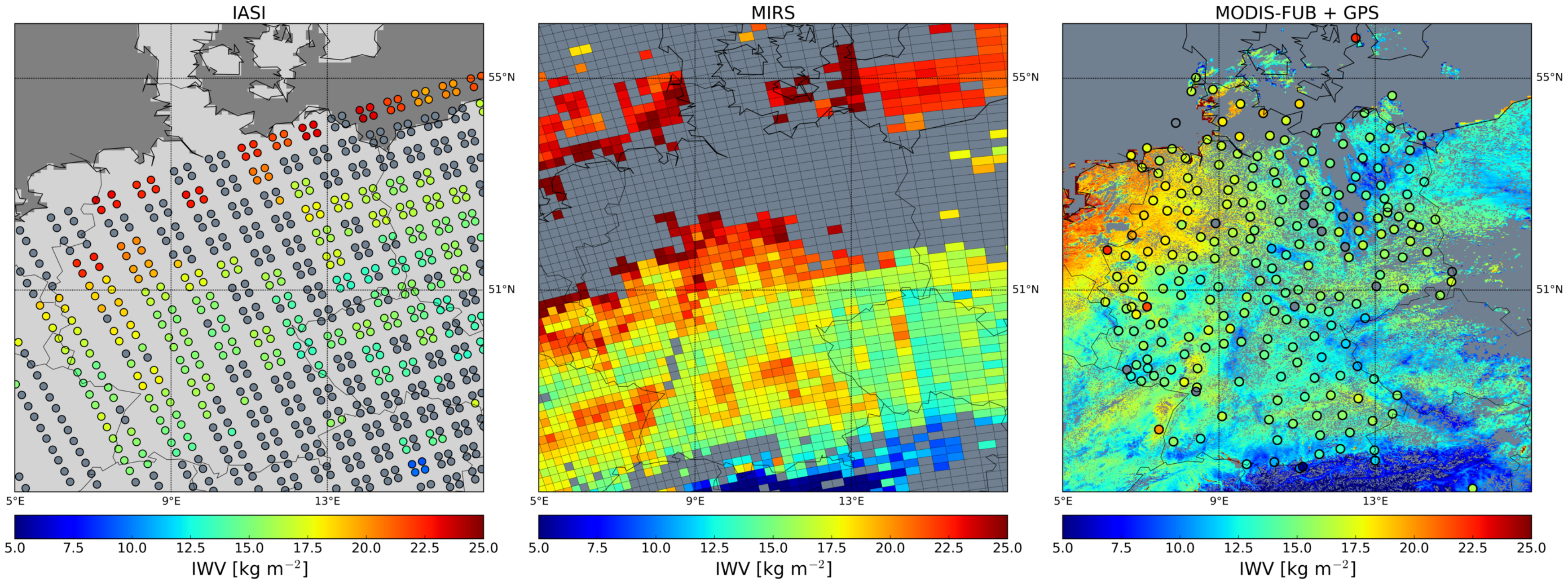
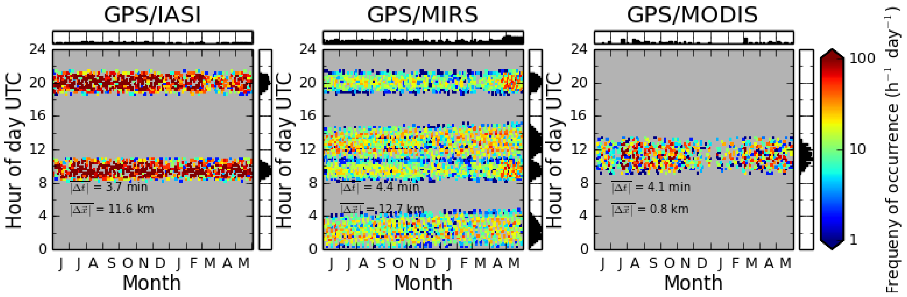
3. Matching Satellite and GPS IWV Measurements

The data sets were collected for a time period of one year, from May 2012 to June 2013 for a predefined German spatial domain (from 5${}^{\circ }$ W to 17${}^{\circ }$ W and from 47${}^{\circ }$ N to 56${}^{\circ }$ N).

The satellite IWV products were all provided as orbital data on a pixel-basis and were cut to the German domain. Before matching the satellite measurements with the GPS measurements, a quality check was applied to the GPS data, also with the help of comparisons with reanalysis simulations from the model COSMO-REA2 [36], to exclude erroneous stations due to, e.g., wrong meteorological data or receiver problems [37]. Also, GPS stations for which the area of 20 km radius around the station consists of more than 10% water surfaces, e.g., lakes, were not used. Together, this resulted in about 160 GPS stations from which IWV data is used in this study. Additionally, the corresponding SEVIRI mean cloud fraction, taking the SEVIRI 15 min time step closest to each GPS measurement time, was stored.

For each satellite overpass, one satellite pixel was attributed to each GPS station to create data pairs of corresponding satellite and GPS IWV values, taking into account several conditions. The pixel with a valid IWV retrieval that is closest to the GPS station is taken and must be located within an area with a radius of 20 km of the GPS station. The radius was chosen such that one can assume the measured IWV at the GPS station to be representative of the water vapor field within the surroundings of the station, while at the same time collecting a large number of satellite-GPS matches for proper statistical results. In this sense, it is a trade-off between exact coincidence in space and statistical significance of the match-up datasets. Furthermore, the time difference between the satellite measurement and the GPS measurement must be within 7.5 min, which basically means the closest GPS time step is taken.

After collection of the satellite-GPS matches, additional filtering was performed. For MODIS, cases with cloud fraction of 50% or higher were filtered out, using the accompanying MODIS 1 km cloud mask, to decrease the probability of including the impact of clouds on, and therefore likely erroneous, retrieved IWV values. Also, cases with MODIS IWV values higher than 50 kg/m${}^2$ were filtered out to prevent the use of, for this spatial domain, unrealistically high IWV values due to retrieval issues, e.g., miss-classified water surfaces. Moreover, all cases where the height difference between the GPS station and the height of the location of the satellite pixel is 100 m or larger, were filtered out. For this, the free Digital Elevation Model (DEM) from NASA’s Shuttle Radar Topography Mission (SRTM) [38] with a spatial resolution of 83 m was used. The height of a satellite pixel was determined by computing the mean height within the pixel size. The mean height difference for all matched cases ranges between 3 m and 5 m for all satellite instruments, and therefore no impact of height difference on the statistical results, presented in the next section, is expected. The filtering removed about 21%, 35% and 19% of the matched cases for IASI, MIRS and MODIS, respectively.

Figure 2 shows the temporal sampling of all matched IASI, MIRS and MODIS measurements with the selected GPS stations throughout the one-year time period. This means the overpass times of the corresponding satellites over the region of interest for which IWV retrievals can be performed and matched to GPS measurements. For all instruments, numerous matched cases can be found in the morning time between 9 h and 11 h UTC, while for IASI and MIRS there are also a large amount of cases in the evening and night time due to the type of measurements, i.e., microwave radiation, used in the algorithms allowing night time retrievals. The slightly higher amount of matched cases for MIRS towards the end of the time period is related to satellite Metop-B, with a morning orbit, becoming operational in April 2013. The lower amount of matched cases for MODIS during the wintertime can be attributed to a higher amount of cloudy to overcast cases, which are not considered, as well as snow-filled pixels misidentified as cloudy.

4. Results

The comparisons and analyses of the satellite and GPS IWV datasets are performed in several ways. First, direct comparisons of the matched and valid satellite-GPS IWV data pairs are shown. However, in many if not most studies IWV climatologies are used, often in the form of monthly means. Therefore, also comparisons of satellite and GPS IWV monthly means are presented. Last, the impact of temporal, spatial and retrieval-specific sampling on the various IWV datasets is investigated to assess and quantify the effect of various sampling issues on resulting aggregated IWV as well as IWV frequency distributions.

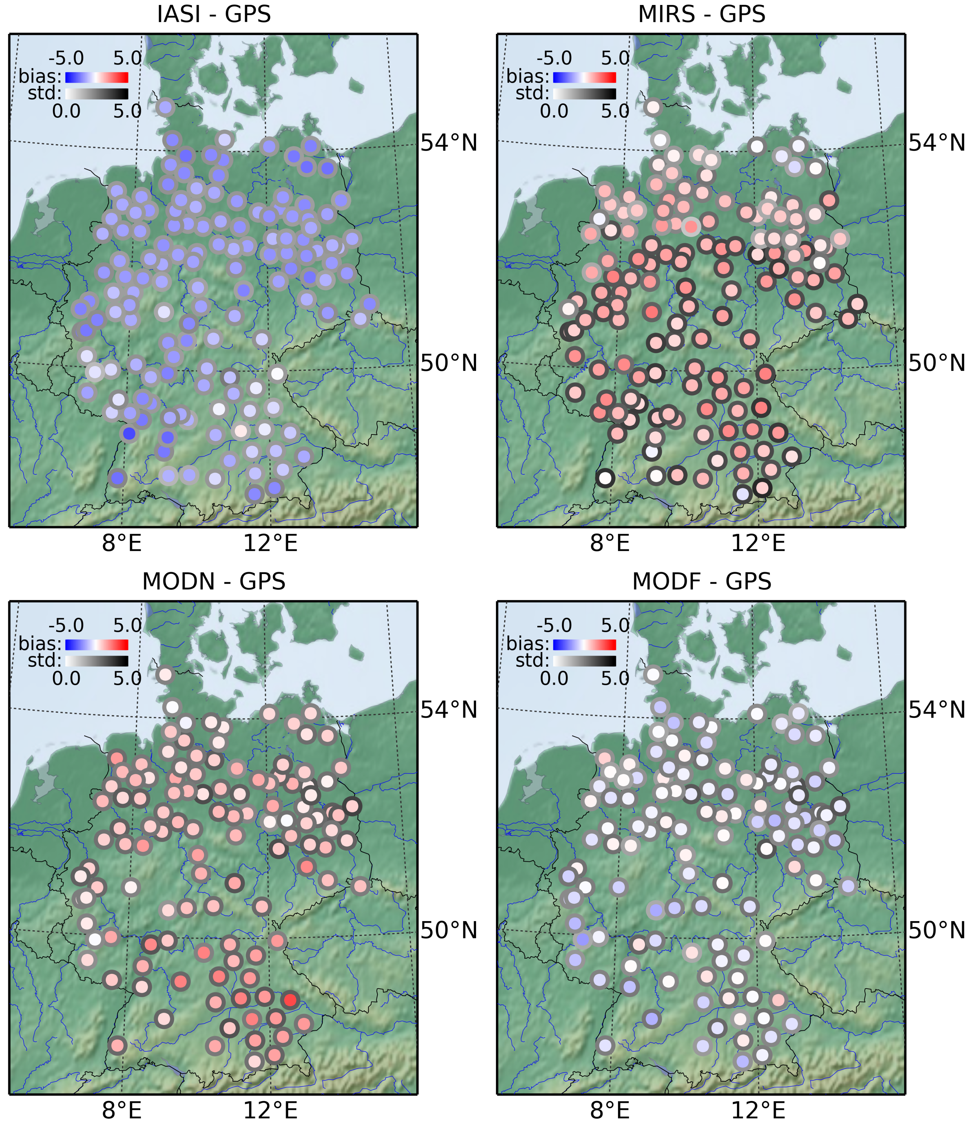
4.1. Direct Comparisons of Satellite and GPS IWV Values

As a first step, all matched and valid IWV cases for the entire German domain and one-year time period are analyzed and the satellite and GPS IWV values are directly compared. Figure 3 shows the frequency of occurrence of all matched and valid satellite-GPS IWV data pairs for each satellite instrument. Statistical quantities related to these comparisons are presented in

Table 2. Statistical quantities computed from the comparison shown in Figure 3. Presented are the number of matched measurements N, bias, root mean square error (RMSE) and standard deviation (STD) of the difference between the IWV dataset from GPS and satellite, the correlation (R) between GPS and each satellite IWV dataset and the slope and intercept of the linear fit shown by the dashed red-blue line in Figure 3. Units of bias, RMSE, Std, Mean(x), Mean(y) and Intercept are given in kg/m${}^2$.

Instrument	N	Bias	RMSE	Std	Mean (x)	Mean (y)	R	Slope	Intercept
IASI	88336	−1.77 ± 0.006	2.74	2.09	16.17	14.40	0.959	0.866 ± 0.001	0.387 ± 0.015
MIRS	41948	1.36 ± 0.016	3.77	3.50	15.98	17.36	0.881	0.807 ± 0.002	4.453 ± 0.037
MODIS	17438	1.11 ± 0.021	3.11	2.91	16.18	17.28	0.959	1.117 ± 0.003	−0.781 ± 0.046
MODIS-FUB	17437	−0.31 ± 0.019	2.52	2.50	16.18	15.87	0.955	0.967 ± 0.002	0.226 ± 0.041

. The 2D histograms and accompanying statistical quantities show that the largest scatter and root mean square error (RMSE) can be seen in the MIRS-GPS comparison, while the lowest scatter and RMSE can be found for the MODIS-FUB-GPS comparison. The range of IWV values, both towards low and high IWV values, is largest in both MODIS-GPS and MODIS-FUB-GPS comparisons, while it is smallest in the IASI-GPS comparison. For the IWV datasets from IASI, MODIS and MODIS-FUB as well as for the corresponding IWV datasets from GPS, a maximum IWV can be seen between 5 and 10 kg/m${}^2$. For MIRS, this maximum can be seen at around 18 kg/m${}^2$. For the corresponding GPS IWV datasets in the IASI, MODIS and MODIS-FUB comparisons also a second maximum around 14 kg/m${}^2$ can be seen. This bi-modal distribution can be observed for MODIS-FUB and IASI as well, and in a lesser extent also for MODIS. The slightly lower second maximum for MODIS and MODIS-FUB compared to GPS is likely related to undetected sub-pixel cloudiness, which results in lower retrieved IWV values.

Comparing the distributions of both MODIS IWV products with IASI and MIRS more extreme IWV values for the former can be seen, related to the higher spatial resolution. Due to the lower spatial resolution of IASI and MIRS, the IWV is smeared out over a larger satellite pixel, thus smoothing out extreme values. The IASI linear fit shows a clear deviation from GPS, resulting in an overall bias of −1.77 kg/m${}^2$. For MIRS, there is a clear overestimation for IWV values until about 25 kg/m${}^2$, which switches to an underestimation at higher IWV values, which are less frequent, resulting in an overall bias of 1.36 kg/m${}^2$. For MODIS, there is an overestimation of IWV values, which increases for higher IWV values, resulting in an overall bias of 1.11 kg/m${}^2$. For MODIS-FUB, there is a minimal underestimation for larger IWV values, resulting in an overall small negative bias of −0.31 kg/m${}^2$.

In a next step, a direct comparison of satellite and GPS IWV values is performed at each GPS station to analyze the spatial distribution of bias and standard deviation within the German domain, see Figure 4. For this, only GPS stations are included for which at least 20 valid satellite-GPS data pairs in the one-year time period where found. Figure 4 shows that no clear geographical distribution of bias can be observed, though the bias and standard deviation can be quite different for ‘neighboring’ GPS stations. In general, the results are dominated by the overall positive or negative bias for each satellite instrument. Furthermore, no clear relationship between bias and standard deviation is observed, though it appears that stations with a higher, absolute bias usually correspond to higher standard deviations. However, the lowest standard deviations appear to be concentrated in the lowlands of Northern Germany, which can be at least partly explained by the flat geography of the region reducing retrieval errors due to height variations within one satellite pixel as well as reducing the impact of height differences between satellite pixel and GPS station on the comparison. The overall mean bias and mean standard deviation are −1.73 kg/m${}^2$ and 2.01 kg/m${}^2$, 1.19 kg/m${}^2$ and 3.03 kg/m${}^2$, 1.12 kg/m${}^2$ and 2.81 kg/m${}^2$, and −0.31 kg/m${}^2$ and 2.41 kg/m${}^2$, for IASI, MIRS, MODIS, and MODIS-FUB, respectively.

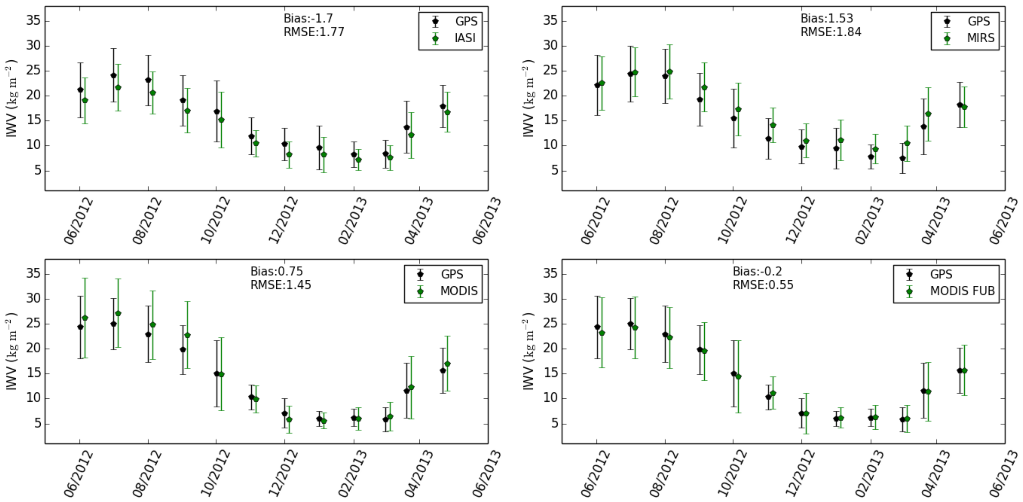
4.2. Comparisons of Satellite and GPS IWV Monthly Means

From the satellite and GPS IWV values of all matched and valid satellite-GPS cases within the German domain climatologies were computed in the form of monthly means. The monthly means were produced by spatially and temporally aggregating all valid IWV values within a one-month time period. Figure 5 shows the annual cycle of IWV, in the form of monthly means and accompanying standard deviations for the IWV dataset from each satellite instrument and the corresponding GPS IWV dataset. IWV shows a maximum in July and a minimum in February-March, except for MODIS, which shows the lowest value in January. Also, for all datasets the absolute standard deviation is highest in the summertime and lowest in the wintertime. The overall biases found before, are naturally also reflected in the monthly mean comparisons. IASI shows an underestimation of IWV for all months. In an absolute sense, the agreement is better in winter than in summer, resulting in an overall bias of −1.7 kg/m${}^2$ and a RMSE of 1.77 kg/m${}^2$. The monthly standard deviations compare well with the GPS standard deviations. MIRS shows a good agreement in the summertime and an overestimation in the wintertime. The standard deviations compare well throughout the year. The overall bias is 1.53 kg/m${}^2$ and the RMSE is 1.84 kg/m${}^2$. MODIS and MODIS-FUB show larger seasonal amplitudes and larger standard deviations than IASI and MIRS, reflecting the more observed extreme IWV values related to a higher spatial resolution. For MODIS, the IWV is overestimated in the summertime, where also the standard deviation is larger than the GPS standard deviation, and slightly underestimated in the wintertime, where the standard deviations are in better agreement. The bias is 0.75 kg/m${}^2$ and the RMSE is 1.45 kg/m${}^2$. The best match can be found for MODIS-FUB. In the summertime there is a slight underestimation of IWV, while in the wintertime the mean IWV values agree best. Throughout the year, the standard deviation is generally slightly larger than the GPS standard deviation. The bias is −0.2 kg/m${}^2$ and the RMSE is 0.55 kg/m${}^2$.

IWV climatologies can be computed for different time scales, e.g., days to seasons. To assess the impact of averaging time period on the computed satellite-based IWV climatologies and their difference to the corresponding GPS climatologies, the bootstrap technique was used. This means that from each IWV dataset all available IWV values belonging to 10,000 averaging time periods, randomly obtained from the one-year IWV dataset, were collected and averaged. Figure 6 shows the results in terms of mean satellite-GPS IWV difference as a function of averaging time period for three different settings. The reference climatology from which the mean IWV difference (error) always is computed is the GPS climatology for which all valid 15 min IWV values within each averaging time period are used. Various satellite-based climatologies are compared to the GPS climatologies.

First, the satellite-based climatologies are computed using the GPS IWV values for all matched satellite pixels (Figure 6 left panel). This was done to ignore the impact of satellite retrieval issues on the results, but only focus on the impact of satellite temporal sampling. All satellite-based climatologies show an underestimation for all averaging time periods. The median ranges from about −0.2 kg/m${}^2$ to −0.5 kg/m${}^2$ for IASI and MIRS, and from about −1.5 kg/m${}^2$ to −2 kg/m${}^2$ for MODIS and MODIS-FUB. The underestimation is thus clearly larger for both MODIS climatologies, which might be related to missing nighttime IWV retrievals and thus lower temporal and possibly stronger biased sampling than IASI and MIRS. The median IWV difference does not change significantly for the various averaging time periods, but appears to be largest around the one to two weeks averaging time. The large confidence intervals, especially for short averaging time periods of days, range from −8 kg/m${}^2$ to 2 kg/m${}^2$, and can be related to the fact that in the German domain the major IWV variability is associated with synoptic disturbances. This also corresponds well with an e-folding time of roughly 13 h that was found from autocorrelation functions for various high temporal IWV measurements obtained during HOPE [18]. However, the confidence intervals decrease significantly for the weekly and monthly averages, naturally related to smoothing due to larger sample sizes.

Second, the mean IWV difference per averaging time period is computed using satellite-based climatologies for which only GPS IWV values are used if matched to a satellite pixel with a successful IWV retrieval (Figure 6 center panel). This also allows investigation of the impact of sampling due to retrieval limitations, such as cloudy conditions for MODIS. Still, the results look very similar to the ones from the first step. The impact of possible lower sampling due to retrieval limitations does hardly affect satellite climatologies computed for any of the averaging time period.

Third, the mean IWV difference per averaging time period is computed using satellite climatologies with actual satellite IWV values (Figure 6 right panel). This allows further investigation of the impact of retrieval bias on satellite climatologies and the difference with GPS climatologies. Now the results have changed significantly. The previously established positive, for MIRS, and negative biases, for IASI, MODIS and MODIS-FUB, dominate the results and not the larger temporal sampling of GPS. The confidence intervals are much larger and vary more in extent between the satellite instruments, which is related to retrieval algorithms and their different limitations. Still, for all satellite instruments, the median values only change very slightly (less than 1 kgm${}^{-2}$) per averaging time period.

4.3. Impact of Temporal and Satellite Retrieval-Specific Sampling on IWV Aggregations and Distributions

The impact of the low temporal sampling of observations from polar-orbiting satellites for the German domain as well as limitations to daytime clear-sky situations on the IWV statistics can be further investigated using the high temporal GPS IWV dataset in combination with the MSG-SEVIRI information on cloud coverage. Figure 7 shows the normalized histograms for all collected 15 min GPS IWV values within the one-year time period as well as for subsets based on daytime (from 9 h to 17 h LT), certain clear-sky (cloud coverage ≤ 0.1), and certain cloudy (cloud coverage ≥ 0.9) cases. Most distributions show a maximum around 8 kg/m${}^2$. However, limitations to daytime and clear-sky cases appear to cause a bi-modal distribution with a first maximum around 5–7 kg/m${}^2$ and a minimum around 9–10 kg/m${}^2$. Also, a relative decline of high IWV values can be noticed. This relates well with the MODIS IWV distributions presented in Figure 3. Overall, the mean IWV and standard deviations for the different subsets vary within 3% of the mean values obtained using all 15 min GPS IWV values. The mean IWV value for the daytime and certain clear-sky cases is the lowest, while considering only daytime and certain cloudy cases has the highest mean IWV value.

The high temporal resolution of the GPS IWV product allows the computation of the mean IWV diurnal cycle for the German domain. Figure 8 shows that the most pronounced mean IWV diurnal cycle is observed in the summertime with an amplitude of about 0.5 kg/m${}^2$. This is related to surface heating due to increasing solar insolation during the day, stimulating convective processes with accompanying transport of moisture into the atmosphere. In the other seasons, the weather conditions and accompanying atmospheric moisture content are even more dominated by large-scale synoptic systems, typical for the mid-latitudes, and thus not necessarily showing a clear diurnal cycle for IWV [37]. This also explains the corresponding large hourly standard deviations, which go up to 6–8 kg/m${}^2$ for all seasons (not shown). The large difference between 00h and 01h LT (23 and 24 UTC) is a known issue of the GPS near-real-time retrieval, which is also seen in the investigations by Steinke et al. [18] as well as in the assessment of the daily cycle at stations in North-America in Dai et al. [39].

To check the representativity of our one-year dataset a longer GPS time series is also considered. Herein, the difference between the one-year IWV diurnal cycle and the one obtained from the years 2007–2013 is only small, especially considering the corresponding large standard deviations. The geographical distribution of the diurnal cycles was also investigated by computing mean IWV diurnal cycles for each GPS station (not shown). Within the German domain, the most pronounced IWV diurnal cycles, i.e., largest amplitudes, were found in the North-eastern part of the domain, which is a flat area near the coast. However, also in this case the magnitude of the standard deviations is much larger than the differences in mean diurnal cycles.

The impact of the reduced temporal sampling of the satellite instruments on computed daily means shows a largest bias for MODIS in the autumn (SON) of about 0.25 kg/m${}^2$. Here, a small diurnal cycle is observed and the MODIS temporal sampling between 10 h and 15 h LT coincides with IWV values that are on average slightly higher than the daily mean. A slightly less pronounced effect can be observed in the summertime, for which also IASI shows a small positive bias of about 0.15 kg/m${}^2$. In general, the satellite overpass times in the late morning and early afternoon (10 h–15 h LT) coincide well with the phase of the IWV mean diurnal cycle that is close to the IWV daily mean. Similar findings for MODIS, but on a global scale, are shown in Diedrich et al. [17]. For IASI and MIRS, the increased temporal sampling at additional daily periods during the evening and nighttime appear to lead to a cancelling out of various deviations from the daily mean, resulting in absolute biases below 0.1 kg/m${}^2$.

Figure 9 shows the impact of temporal sampling and retrieval-specific characteristics/limitations for each satellite instrument, now also making use of the actual satellite IWV values. Compared are distributions and corresponding statistics obtained from (1) IWV values from all GPS timesteps, (2) GPS IWV values for timesteps matched with satellite observations, (3) GPS IWV values for timesteps matched with satellite observations with a valid IWV retrieval, (4) all valid satellite IWV values. Going from step 1 to step 2, i.e., the impact of temporal sampling, leads to a slightly lower frequency of lower IWV value and slightly higher frequency of mid-to-high IWV values, thus resulting in a higher mean IWV value. Going to step 3, i.e., including the impact of retrieval limitations such as daytime or clear-sky cases, results in a higher frequency of lower IWV values as well as in a lower frequency of higher IWV values. For MODIS and IASI this could be related to the filtering out of cloudy cases, which are related to higher IWV values, see Figure 7. Now both MODIS retrievals also show a much clearer bi-modal distribution with a minimum around 9–10 kg/m${}^2$, which corresponds well with the result presented in Figure 7 for the IWV distribution under daytime and clear-sky conditions. Going to step 4, i.e., considering the performance of the satellite retrieval algorithms, the difference to step 1 becomes largest for all instruments showing that the overall retrieval bias has the largest impact on the distributions and its corresponding statistics. IASI shows a much lower number of higher IWV values, while MIRS misses many lower IWV values. This ’smoothing’ is related to the large satellite pixel sizes of the instruments and is also reflected in the lower standard deviations. MODIS-FUB still shows a clear bi-modal distribution, while for MODIS the second bump is smoothed out and shows a much larger number of higher IWV values resulting in a clear wet bias.

We have seen that while the shape of IWV distributions can change significantly due to changes in sampling method, the mean values only show minor changes. The limitations of daytime and clear-sky cases do not seem to impact mean results significantly. More specifically, the low temporal sampling of the satellite instruments and retrieval-specific limitations only lead to small biases of −0.06 kg/m${}^2$, −0.25 kg/m${}^2$, −0.05 kg/m${}^2$ and −0.05 kg/m${}^2$ for IASI, MIRS, MODIS and MODIS-FUB, respectively. The overall biases, obtained by comparing directly all matched GPS and satellite IWV values, are much larger, indicating that the impact of the performance of the retrieval algorithms clearly dominates in the mean statistics.

However, a closer look at the statistics listed in

Table 3. Summary of difference between average GPS IWV obtained from various sampling methods and average GPS IWV obtained from all GPS time steps and all GPS stations ($\mathsf{\Delta }$IWV in kg/m${}^2$). Results are shown for the average computed from all relevant IWV values ($\overline{All}$), the 10th, 50th and 90th percentiles and for the averages computed from all relevant IWV values within the periods June-August ($\overline{JJA}$), September-November ($\overline{SON}$), December-February ($\overline{DJF}$) and March-May ($\overline{MAM}$). Numbers within brackets indicate the relative frequency of IWV values with respect to the complete time period of one year. Please note that the relative frequency of IWV values from all GPS time steps and all stations with respect to the complete time period of one year is about 25% for each season.

$\mathbf{\Delta }$IWV	$\overline{\mathit{All}}$	10%	50%	90%	$\overline{\mathit{JJA}}$	$\overline{\mathit{SON}}$	$\overline{\mathit{DJF}}$	$\overline{\mathit{MAM}}$
Certain clear sky	0.24	0.10	0.70	−0.50	−1.83 (33.7%)	−1.24 (33.5%)	−0.89 (13.7%)	−1.19 (19.1%)
Daytime	0.12	−0.10	0.20	0.20	0.15 (25.2%)	0.05 (25.0%)	0.09 (24.1%)	−0.14 (25.7%)
Daytime & certain clear sky	−0.01	−0.80	0.50	−0.20	−1.20 (31.0%)	−1.31 (35.5%)	0.25 (11.5%)	−3.06 (22.0%)

and

Table 4. Summary of difference between average GPS IWV obtained from satellite sampling (GPS with satellite sampling) as well as average satellite IWV (Bias) and average GPS IWV obtained from all GPS time steps and all GPS stations ($\mathsf{\Delta }$IWV in kg/m${}^2$). Results are shown for the average computed from all IWV values ($\overline{All}$), the 10th, 50th and 90th percentiles and for the averages computed from all IWV values within the periods June-August ($\overline{JJA}$), September-November ($\overline{SON}$), December-February ($\overline{DJF}$) and March-May ($\overline{MAM}$). Numbers within brackets indicate the relative frequency of IWV values with respect to the complete time period of one year. Please note that the relative frequency of IWV values from all GPS time steps and all stations with respect to the complete time period of one year is about 25% for each season.

$\mathbf{\Delta }$IWV	$\overline{\mathit{All}}$	10%	50%	90%	$\overline{\mathit{JJA}}$	$\overline{\mathit{SON}}$	$\overline{\mathit{DJF}}$	$\overline{\mathit{MAM}}$
GPS with IASI sampling	−0.05	0.50	0.00	−1.10	−1.28 (28.8%)	−0.90 (29.7%)	−0.70 (23.1%)	0.45 (18.4%)
IASI Bias	−1.83	−0.28	−1.48	−3.79	−3.66	−2.62	−2.25	−0.74
GPS with MIRS sampling	−0.25	−0.10	0.30	−1.11	−0.83 (24.0%)	−1.29 (24.6%)	−1.07 (18.4%)	0.79 (33.0%)
MIRS Bias	1.12	1.90	1.70	−0.81	−0.26	1.01	0.45	2.05
GPS with MODIS sampling	−0.05	−1.20	0.30	0.49	−0.41 (31.5%)	−0.93 (32.3%)	−3.44 (7.9%)	−3.24 (28.3%)
MODIS Bias	1.06	−1.35	1.20	3.85	1.53	0.07	−4.23	−2.40
MODIS-FUB Bias	−0.36	−1.46	−0.11	0.49	−1.23	−1.11	−3.36	−3.24

, corresponding to the distributions shown in Figure 7 and Figure 9, respectively, reveal that for various subsets of the IWV datasets the IWV differences can be as large or even larger than the overall biases obtained from the one-year time period. The 10, 50 and 90 percentiles show that while the overall mean IWV difference is positive/negative, the IWV difference at low, median and high IWV values can be negative/positive. This demonstrates that a mean IWV value is not necessarily representative for the entire IWV distribution. The same can be said for seasonal IWV subsets. For example, while the overall mean IWV difference between the GPS IWV obtained for daytime and certain clear-sky cases and all GPS time steps is nearly zero, the mean IWV difference for the spring period is −3.06 kg/m${}^2$, see Table 3. Table 4 shows that the overall mean IWV difference is clearly smaller using the GPS IWV values with satellite sampling, compared to using the actual satellite IWV values (satellite bias), while this is not necessarily true at the low (10th percentile) and high (90th percentile) end of the IWV distributions. On a seasonal basis, the mean IWV differences can be much larger than the overall satellite bias. The largest IWV difference of −4.23 kg/m${}^2$ is found for MODIS in the winter time, which will be related to both low sampling conditions due to high cloud coverage as well as challenging retrieval conditions due to high solar zenith angles and snow covered surfaces.

5. Discussion

This study provides an assessment of various well-established integrated water vapor products from several passive instruments on polar-orbiting satellites using measurements from a one-year time period, from June 2012 to May 2013, for a German domain. The instrument characteristics differ in spectral channels, spatial resolution and overpass times, while the corresponding IWV retrieval algorithms are subject to different types of limitations such as daytime and clear-sky situations. The quantification of the impact of the temporal sampling and retrieval-specific limitations on pixel-based IWV products as well as aggregated IWV data is performed using IWV measurements from the dense German GPS network as a reference dataset. The satellite IWV products under consideration are based on data from IASI, MIRS, and MODIS.

The direct comparison of IWV values for each satellite instrument with the corresponding GPS IWV values reveal an overall bias of 1.77, 1.36, 1.11 and −0.31 kg/m${}^2$ for IASI, MIRS, MODIS and MODIS-FUB, respectively. All instrument and GPS distributions show the most frequent occurrence of IWV around 8 kg/m${}^2$, except MIRS. Both IASI and MIRS show narrower distributions, related to the large satellite pixel sizes of 12 km and 16 km, going up to about 40 km and 50 km at swath edge, respectively, which smooth out extreme IWV values. The distributions of MODIS and MODIS-FUB show the clearest bi-model shape. A direct comparison performed at each GPS station separately does not show a clear geographical distribution of mean and standard deviations of IWV differences, except for a tendency for somewhat lower standard deviations in Northern Germany, which is a flat region. This might be attributed to a low impact of height variations within a satellite pixel as well as of height differences between satellite pixel and GPS station.

From the pixel-based IWV products, aggregated statistics were computed in the form of monthly means and compared to the GPS. In general, the annual cycle and corresponding standard deviations are well represented for all instruments. Overall biases obtained earlier are also reflected in the monthly means, thus a best match with GPS was found for MODIS-FUB. Different averaging time periods, going from 1 day to 3 months, hardly influence the difference between mean satellite-based IWV and mean IWV obtained from all 15 min GPS time steps within an averaging time period. This is related to the fact that in Germany the IWV fields and their temporal variability are dominated by large synoptic disturbances occurring on the time scale of about one day.

With the use of the GPS IWV product in combination with a SEVIRI cloud coverage product, both on 15 min temporal resolution, the impact of retrieval-specific limitations on IWV distributions and corresponding statistics is assessed. The distributions change into a bi-modal distribution when only daytime and certain clear-sky cases are considered, which fits well with the MODIS bi-modal distributions observed earlier. Also, a loss of high IWV values is observed. From the GPS IWV product, a mean diurnal cycle and satellite-based daily means are computed to assess the impact of the low temporal sampling of instruments on polar-orbiting satellites on mean IWV. The satellite temporal sampling hardly leads to any biases, since the overpass times in the late morning/early afternoon are located around or close to the daily mean for MODIS or, in combination with the night time overpasses, appear to cancel each other out for IASI and MIRS. In addition, the amplitude of the mean diurnal cycle is small, about 0.5 kg/m${}^2$ for the summer time (highest amplitude), especially when compared to the corresponding standard deviations of about 8 kg/m${}^2$, related to the dominance of the noisy large-scale weather systems in Germany. However, when weather anomalies occur larger differences can be expected as fair-weather conditions introduce much stronger daily amplitudes [37].

Combining the validation results with the results of the impact of sampling issues on IWV, temporal and retrieval-specific, show that sampling effects affect mean IWV values only marginally. The overall IWV differences/biases are dominated by the performance of the retrieval algorithms. This is also reflected in the difference in performance of both MODIS IWV products, which use the same measurements, but different retrieval algorithms. However, sampling affects the shape of IWV distributions, e.g., observed with the bi-modal IWV distribution for MODIS and loss of high IWV values, while for IASI and MIRS, the low spatial resolution leads to even stronger smoothing of IWV values. A closer look at several statistics on IWV differences, corresponding to the analyzed distributions, such as the 10th, 50th and 90th percentile as well as mean seasonal differences, reveals that differences at low and high IWV values as well as a mean seasonal IWV difference can become significantly larger than the overall IWV bias, though the results differ notably per sampling method and satellite retrieval algorithm.

While this study helps us to further understand the performances and limitations of the various satellite IWV products over a region of structured terrain in Central-Europe, the results are not necessarily applicable to other regions in the world, especially if dominated by other types of weather conditions. In very cloudy regions, a MODIS IWV climatology could possess a significant bias, while it could become problematic for IASI and MIRS IWV retrievals in very wet or dry regions with extreme low or high IWV values. In a next step, the study can be extended globally making use of the increasing number of worldwide GNSS stations, which covers various climate regions, relevant for climate studies. It would naturally also benefit from including IWV products from other types of instruments/measurements as well. Furthermore, many IWV retrievals and corresponding datasets are under constant development, thus making it preferable to repeat these kinds of analyses on a regular basis and along the process including newly developed IWV datasets. Of particular interest for the impact assessment of spatial sampling on retrieved IWVs could be the inclusion of the newly developed high spatial resolution IWV product (≈300 m) from the Ocean and Land Color Instrument (OLCI) on the polar-orbiting satellite Sentinel-3 [40,41].

References

1. Kiehl, J.T.; Trenberth, K.E. Earth’s annual global mean energy budget. Bull. Am. Meteorol. Soc. 1997, 78, 197–208. [Google Scholar] [CrossRef] [Green Version]
2. Bengtsson, L. The global atmospheric water cycle. Environ. Res. Lett. 2010, 5, 025202. [Google Scholar] [CrossRef]
3. Held, I.M.; Soden, B.J. Water vapor feedback and global warming. Annu. Rev. Energy Environ. 2000, 25, 441–475. [Google Scholar] [CrossRef] [Green Version]
4. Lacis, A.A.; Schmidt, G.A.; Rind, D.; Ruedy, R.A. Atmospheric CO2: Principal control knob governing Earth’s temperature. Science 2010, 330, 356–359. [Google Scholar] [CrossRef] [Green Version]
5. Hegerl, G.C.; Black, E.; Allan, R.P.; Ingram, W.J.; Polson, D.; Trenberth, K.E.; Chadwick, R.S.; Arkin, P.A.; Sarojini, B.B.; Becker, A.; et al. Challenges in quantifying changes in the global water cycle. Bull. Am. Meteorol. Soc. 2019, 100. [Google Scholar] [CrossRef] [Green Version]
6. Bony, S.; Duvel, J.P.; Le Trent, H. Observed dependence of the water vapor and clear-sky greenhouse effect on sea surface temperature: Comparison with climate warming experiments. Clim. Dyn. 1995, 11, 307–320. [Google Scholar] [CrossRef]
7. Jiang, J.H.; Su, H.; Zhai, C.; Perun, V.S.; Del Genio, A.; Nazarenko, L.S.; Donner, L.J.; Horowitz, L.; Seman, C.; Cole, J.; et al. Evaluation of cloud and water vapor simulations in CMIP5 climate models using NASA “A-Train” satellite observations. J. Geophys. Res. Atmos. 2012, 117. [Google Scholar] [CrossRef] [Green Version]
8. Stevens, B.; Brogniez, H.; Kiemle, C.; Lacour, J.L.; Crevoisier, C.; Kiliani, J. Structure and dynamical influence of water vapor in the lower tropical troposphere. In Shallow Clouds, Water Vapor, Circulation, and Climate Sensitivity; Springer: Berlin, Germany, 2017; pp. 199–225. [Google Scholar]
9. Durre, I.; Vose, R.S.; Wuertz, D.B. Overview of the integrated global radiosonde archive. J. Clim. 2006, 19, 53–68. [Google Scholar] [CrossRef] [Green Version]
10. Mears, C.A.; Smith, D.K.; Ricciardulli, L.; Wang, J.; Huelsing, H.; Wentz, F.J. Construction and uncertainty estimation of a satellite-derived total precipitable water data record over the world’s oceans. Earth Space Sci. 2018, 5, 197–210. [Google Scholar] [CrossRef] [Green Version]
11. Rinke, A.; Segger, B.; Crewell, S.; Maturilli, M.; Naakka, T.; Nygård, T.; Vihma, T.; Alshawaf, F.; Dick, G.; Wickert, J.; et al. Trends of Vertically Integrated Water Vapor over the Arctic during 1979–2016: Consistent Moistening All Over? J. Clim. 2019, 32, 6097–6116. [Google Scholar] [CrossRef]
12. Chahine, M.T. GEWEX: The global energy and water cycle experiment. Eos Trans. Am. Geophys. Union 1992, 73, 9–14. [Google Scholar] [CrossRef]
13. Schröder, M.; Lockhoff, M.; Shi, L.; August, T.; Bennartz, R.; Borbas, E.; Brogniez, H.; Calbet, X.; Crewell, S.; Eikenberg, S.; et al. GEWEX Water Vapor Assessment (G-VAP); WCRP Report 16/2017; World Climate Research Programme (WCRP): Geneva, Switzerland, 2017. [Google Scholar]
14. Carbajal Henken, C.; Diedrich, H.; Preusker, R.; Fischer, J. MERIS full-resolution total column water vapor: Observing horizontal convective rolls. Geophys. Res. Lett. 2015, 42, 10–074. [Google Scholar] [CrossRef]
15. Sohn, B.J.; Bennartz, R. Contribution of water vapor to observational estimates of longwave cloud radiative forcing. J. Geophys. Res. Atmos. 2008, 113. [Google Scholar] [CrossRef]
16. Roman, J.; Knuteson, R.; August, T.; Hultberg, T.; Ackerman, S.; Revercomb, H. A global assessment of NASA AIRS v6 and EUMETSAT IASI v6 precipitable water vapor using ground-based GPS SuomiNet stations. J. Geophys. Res. Atmos. 2016, 121, 8925–8948. [Google Scholar] [CrossRef]
17. Diedrich, H.; Wittchen, F.; Preusker, R.; Fischer, J. Representativeness of total column water vapour retrievals from instruments on polar orbiting satellites. Atmos. Chem. Phys. 2016, 16, 8331–8339. [Google Scholar] [CrossRef] [Green Version]
18. Steinke, S.; Eikenberg, S.; Löhnert, U.; Dick, G.; Klocke, D.; Di Girolamo, P.; Crewell, S. Assessment of small-scale integrated water vapour variability during HOPE. Atmos. Chem. Phys. 2015, 15, 2675–2692. [Google Scholar] [CrossRef] [Green Version]
19. Macke, A.; Seifert, P.; Baars, H.; Barthlott, C.; Beekmans, C.; Behrendt, A.; Bohn, B.; Brueck, M.; Bühl, J.; Crewell, S.; et al. The HD (CP) 2 Observational Prototype Experiment (HOPE)—An overview. Atmos. Chem. Phys. 2017, 17, 4887–4914. [Google Scholar] [CrossRef] [Green Version]
20. Schmetz, J.; Pili, P.; Tjemkes, S.; Just, D.; Kerkmann, J.; Rota, S.; Ratier, A. An introduction to Meteosat second generation (MSG). Bull. Am. Meteorol. Soc. 2002, 83, 977–992. [Google Scholar] [CrossRef]
21. Gendt, G.; Dick, G.; Reigber, C.; Tomassini, M.; Liu, Y.; Ramatschi, M. Near real time GPS water vapor monitoring for numerical weather prediction in Germany. J. Meteorol. Soc. 2004, 82, 361–370. [Google Scholar] [CrossRef] [Green Version]
22. August, T.; Klaes, D.; Schlüssel, P.; Hultberg, T.; Crapeau, M.; Arriaga, A.; O’Carroll, A.; Coppens, D.; Munro, R.; Calbet, X. IASI on Metop-A: Operational Level 2 retrievals after five years in orbit. J. Quant. Spectrosc. Radiat. Transf. 2012, 113, 1340–1371. [Google Scholar] [CrossRef]
23. Boukabara, S.A.; Garrett, K.; Chen, W.; Iturbide-Sanchez, F.; Grassotti, C.; Kongoli, C.; Chen, R.; Liu, Q.; Yan, B.; Weng, F.; et al. MiRS: An all-weather 1DVAR satellite data assimilation and retrieval system. IEEE Trans. Geosci. Remote Sens. 2011, 49, 3249–3272. [Google Scholar] [CrossRef]
24. Gao, B.; Kaufman, Y.J. Water vapor retrievals using moderate resolution imaging spectroradiometer (MODIS) near-infrared channels. J. Geophys. Res. Atmos. 2003, 108, D13. [Google Scholar] [CrossRef]
25. Diedrich, H.; Preusker, R.; Lindstrot, R.; Fischer, J. Retrieval of daytime total columnar water vapour from MODIS measurements over land surfaces. Atmos. Meas. Tech. 2015, 8, 823–836. [Google Scholar] [CrossRef] [Green Version]
26. Fang, P.; Bevis, M.; Bock, Y.; Gutman, S.; Wolfe, D. GPS meteorology: Reducing systematic errors in geodetic estimates for zenith delay. Geophys. Res. Lett. 1998, 25, 3583–3586. [Google Scholar] [CrossRef]
27. Steinke, S. Variability of Integraded Water Vapor: An Assessment on Various Scales with Observations and Model Simulations over Germany. Ph.D. Thesis, University of Cologne, Cologne, Germany, 2017. [Google Scholar]
28. Ning, T.; Wang, J.; Elgered, G.; Dick, G.; Wickert, J.; Bradke, M.; Sommer, M. The uncertainty of the atmospheric integrated water vapour estimated from GNSS observations. Atmos. Meas. Tech. 2016, 9, 79–92. [Google Scholar] [CrossRef] [Green Version]
29. Zhang, D.; Guo, J.; Chen, M.; Shi, J.; Zhou, L. Quantitative assessment of meteorological and tropospheric Zenith Hydrostatic Delay models. Adv. Space Res. 2016, 58, 1033–1043. [Google Scholar] [CrossRef]
30. Dick, G.; Gendt, G.; Reigber, C. First experience with near real-time water vapor estimation in a German GPS network. J. Atmos. Sol.-Terr. Phys. 2001, 63, 1295–1304. [Google Scholar] [CrossRef]
31. NOAA Center for Satellite Applications and Research (STAR). Available online: https://www.star.nesdis.noaa.gov/mirs/downloaddap.php (accessed on 10 January 2020).
32. NASA Level-1 and Atmosphere Archive & Distribution System (LAADS) Distributed Active Archive Center (DAAC). Available online: https://ladsweb.nascom.nasa.gov/ (accessed on 10 January 2020).
33. Lindstrot, R.; Preusker, R.; Diedrich, H.; Doppler, L.; Bennartz, R.; Fischer, J. 1D-Var retrieval of daytime total columnar water vapour from MERIS measurements. Atmos. Meas. Tech. 2012, 5, 631. [Google Scholar] [CrossRef] [Green Version]
34. Reuter, M.; Thomas, W.; Albert, P.; Lockhoff, M.; Weber, R.; Karlsson, K.G.; Fischer, J. The CM-SAF and FUB cloud detection schemes for SEVIRI: Validation with synoptic data and initial comparison with MODIS and CALIPSO. J. Appl. Meteorol. Climatol. 2009, 48, 301–316. [Google Scholar] [CrossRef]
35. Rathke, C.; Fischer, J. Retrieval of cloud microphysical properties from thermal infrared observations by a fast iterative radiance fitting method. J. Atmos. Ocean. Technol. 2000, 17, 1509–1524. [Google Scholar] [CrossRef]
36. Wahl, S.; Bollmeyer, C.; Crewell, S.; Figura, C.; Friederichs, P.; Hense, A.; Keller, J.D.; Ohlwein, C. A novel convective-scale regional reanalysis COSMO-REA2: Improving the representation of precipitation. Meteorol. Z. 2017, 26, 345–361. [Google Scholar] [CrossRef]
37. Steinke, S.; Wahl, S.; Crewell, S. Benefit of high resolution COSMO reanalysis: The diurnal cycle of column-integrated water vapor over Germany. Meteorol. Z. 2019, 28, 165–177. [Google Scholar] [CrossRef]
38. Farr, T.G.; Kobrick, M. Shuttle Radar Topography Mission produces a wealth of data. Eos Trans. Am. Geophys. Union 2000, 81, 583–585. [Google Scholar] [CrossRef]
39. Dai, A.; Wang, J.; Ware, R.H.; Van Hove, T. Diurnal variation in water vapor over North America and its implications for sampling errors in radiosonde humidity. J. Geophys. Res. Atmos. 2002, 107. [Google Scholar] [CrossRef] [Green Version]
40. Donlon, C.; Berruti, B.; Buongiorno, A.; Ferreira, M.H.; Féménias, P.; Frerick, J.; Goryl, P.; Klein, U.; Laur, H.; Mavrocordatos, C.; et al. The global monitoring for environment and security (GMES) sentinel-3 mission. Remote Sens. Environ. 2012, 120, 37–57. [Google Scholar] [CrossRef]
41. Aguirre, M.; Berruti, B.; Bezy, J.L.; Drinkwater, M.; Heliere, F.; Klein, U.; Mavrocordatos, C.; Silvestrin, P.; Greco, B.; Benveniste, J. Sentinel-3-the ocean and medium-resolution land mission for GMES operational services. ESA Bull. 2007, 131, 24–29. [Google Scholar]
Figure 1. Examples of spatial sampling for IASI, MIRS and MODIS for 24 April 2013 over a German domain, at overpass times of about 19:34 UTC, 20:30 UTC and 12:30 UTC, respectively. On the right are the GPS stations (circles) from the German GPS network used in this study and corresponding IWV values at the MODIS overpass time. For this day IWV products from 236 GPS stations were available. Areas in grey indicate that no (successful) IWV retrievals were performed or obtained.
Remotesensing 12 01170 g001
Figure 2. Temporal sampling of the IASI, MIRS and MODIS instruments at all GPS stations combined for one year, assuming for each satellite overpass a maximum distance of 20 km and a maximum time difference of 7.5 min between satellite pixel and GPS station.
Remotesensing 12 01170 g002
Figure 3. 2D histograms and probability density functions for IWV GPS vs. IWV from IASI, MIRS, MODIS and MODIS-FUB. The dashed black-white diagonal line is the 1:1 line, while the dashed red-blue line presents a linear fit through the data. Corresponding statistical quantities can be found in Table 2.
Remotesensing 12 01170 g003
Figure 4. Bias (inner circle colors ranging from blue to red) and standard deviation (std; outer circle colors in greyish colors) at each GPS station for all matched IWV observations within one year. Only the GPS stations are included with at least 20 valid satellite-GPS data pairs.
Remotesensing 12 01170 g004
Figure 5. Comparison of monthly mean of IWV from GPS to IASI, MIRS, MODIS and MODIS-FUB for all months from June 2012 to May 2013. The error bars show the standard deviation. Bias and root mean square error (RMSE) are given in kg/m 2 .
Remotesensing 12 01170 g005
Figure 6. Averaging time period vs. error (using as reference GPS climatologies computed from all 15 min IWV values within an averaging time period) obtained from bootstrap using a sample size of 10,000 for each averaging time period. The dots show the median and the bars indicate the 5% and 95% confidence levels. Left: for GPS IWV values for all matched satellite pixels. Middle: for GPS IWV values for all matched satellite pixels with successfully retrieved satellite IWV values. Right: satellite IWV values for all matched satellite pixels and successfully retrieved satellite IWV values
Remotesensing 12 01170 g006
Figure 7. IWV distributions for all GPS IWV observations, for all GPS IWV observations during daytime as well as for certain clear-sky and certain cloudy cases.
Remotesensing 12 01170 g007
Figure 8. Hourly deviations from the IWV daily mean (zero black dashed line) computed using all 15 min GPS IWV values from the one-year time period (black line) and using all 15 min GPS IWV values from the years 2007–2013 (grey line). Overlaid are the deviations of the satellite daily means, computed using the GPS IWV values for matched GPS-satellite cases, to the GPS daily mean from the one-year time period (colored horizontal lines). The relative frequency of occurrence of satellite IWV values at corresponding hourly time intervals is shown in the lower parts of the panels. Results are presented for local time (LT) for four seasons: June–July–August (JJA), September–October–November (SON), December–January–February (DJF), March–April–May (MAM).
Remotesensing 12 01170 g008
Figure 9. IWV distributions for GPS IWV values for all GPS time steps (black), for GPS IWV values for all time steps matched with satellite observations (green), for GPS IWV values for all timesteps matched with satellite observations with valid IWV retrieval (blue), and for all matched valid satellite IWV values (red).
Remotesensing 12 01170 g009