Article

Regional Dependence of Atmospheric Responses to Oceanic Eddies in the North Pacific Ocean

1
College of Ocean and Earth Sciences, Xiamen University, Xiamen 361102, China
2
Second Institute of Oceanography, MNR, Hangzhou 310012, China
3
Collaborative Innovation Center on Forecast and Evaluation of Meteorological Disasters, University of Information Science and Technology, Nanjing 210044, China
4
Oceanic Modeling and Observation Laboratory, Nanjing University of Information Science & Technology, Nanjing 210044, China
5
Department of Geography, University of California Berkeley, CA 94720-4740, USA
6
School of Oceanography, Shanghai Jiao Tong University, Shanghai 200000, China
*
Author to whom correspondence should be addressed.
Remote Sens. 2020, 12(7), 1161; https://doi.org/10.3390/rs12071161
Submission received: 28 February 2020 / Revised: 26 March 2020 / Accepted: 1 April 2020 / Published: 4 April 2020
(This article belongs to the Section Ocean Remote Sensing)

Abstract

:
Based on sea surface height anomaly (SSHA) from satellite altimeter and microwave radiometer datasets, this study investigates atmospheric responses to oceanic eddies in four subdomains of the North Pacific Ocean with strongest eddy activity: Kuroshio Extension (KE), Subtropical Front (SF), California Coastal Current (CC) and Aleutian Islands (AI). Analyses show that anticyclonic eddies cause sea surface temperature, surface wind speed and precipitation rate to increase in all four subdomains, and vice versa. Through a further examination of the regional dependence of atmospheric responses to oceanic eddies, it is found that the strongest and the weakest surface wind speed responses (in winter and summer) are observed in the KE and AI region, respectively. For precipitation rate, seasonal variation of the atmospheric responses to oceanic eddies is strongest in winter and weakest in summer in the KE, CC and AI regions, but stronger in summer in the SF area. The reasons for such regional dependence and seasonality are the differences in the strength of SST anomalies, the vertical kinetic energy flux and atmospheric instability in the four subdomains.

Graphical Abstract

1. Introduction

Mesoscale eddies are ubiquitous in oceans globally [1,2,3,4,5,6] and play integral roles in redistributing ocean heat, salt, momentum and nutrients [7,8,9,10,11,12,13,14,15,16,17,18,19,20]. These structures span tens to hundreds of kilometers and can occur from tens to hundreds of days.
Recently available high-resolution satellite measurements of the global ocean and the rapid development of supercomputing resources has led to more intensive mesoscale air–sea interaction research. Extensive research shows that the majority of sea surface temperature anomaly (SSTA) phenomena are associated with oceanic mesoscale processes such as oceanic mesoscale eddies and fronts [2,9,21,22,23]. Several studies [24,25,26,27,28,29,30], using satellite and numerical data to investigate air–sea interactions over mesoscale oceanic eddies and frontal regions, show a high positive correlation between wind speed and SST. Their results are contrary to basin-scale ocean circulation and variation driven by the overlying atmosphere (wind stress), which portray a negative correlation between wind speed and SST in the extratropics. The effects of transient oceanic eddies on the overlying atmosphere are examined in Kuroshio Extension [24], Kuroshio, Gulf Stream, Agulhas Return Current, and Southern Ocean [28,29,30] regions, respectively. In these studies, it is found that cyclonic (anticyclonic) eddies can promote decreases (increases) in SST, wind speed, cloud liquid and precipitation rate. Recent studies also indicate that oceanic frontal-scale variations in some strong current regions impact the marine atmospheric boundary layer (MABL) [29,31], and even the troposphere [21,24,32].
Two primary mechanisms are responsible for sea surface wind responses to SSTA: (1) the vertical mixing mechanism [32,33], in which the near-surface atmosphere becomes unstable over warmer SSTs, thereby inducing an enhanced downward momentum transport from higher up in the atmospheric column and consequently, intensifying surface winds; (2) the sea level pressure (SLP) adjustment mechanism [34], where SST anomalies alter the MABL’s air temperature, resulting in an SLP increase on the cold side. Over warm SST, these low-pressure anomalies generate cyclonic circulation and induce surface wind convergence.
As discussed above, several previous studies have investigated the effects of mesoscale eddies on the overlying atmosphere in specific regions [24,27,28,29,30,31,32,35,36,37], such as Kuroshio Extension [24], Gulf Stream, Agulhas Return Current, Southern Ocean, and Kuroshio [27,28,29,30] regions. Such separate studies do not answer how the oceanic and atmospheric conditions affect the atmospheric response to the oceanic eddies, which is essential to understand the problem fully. In the present study, we chose four areas to investigate how the oceanic eddies impact the atmospheric physical processes under different oceanic and atmospheric conditions. However, studies on the regional dependence of atmospheric responses to oceanic eddies are still lacking. To bridge this gap, we used high-resolution satellite data and a reanalysis product to establish two air–sea coupled mesoscale eddy data sets in four eddy-rich subdomains of the North Pacific Ocean: Kuroshio Extension [KE, (28°N–42°N, 140°E–180°E)], Subtropical Frontal region [SF, (15°N–23°N, 123°E–150°W)], California Coastal Current [CC, (20°N–40°N, 105°W–140°W)] and Aleutian Islands [AI, (48°N–56°N, 165°E–155°W)]. We used the two datasets to examine the regional dependence of atmospheric responses to mesoscale eddies with temporal variations by comparisons among the four subdomains. The underlying mechanisms are also discussed.
The remainder of the present paper is organized as follows: Section 2 introduces the data and method; Section 3 investigates eddy characteristics and atmospheric responses to mesoscale eddies. Section 4 and Section 5 are a discussion of the underlying mechanisms and a summary, respectively.

2. Data and Methods

2.1. SSHA

Archiving, Validation and Interpretation of Satellite Oceanographic (AVISO) produce and distribute altimeter SSHA datasets at a spatial resolution of 1/3° × 1/3° and a weekly time resolution. Data covering 2002–2010 in the four North Pacific subdomains are used.

2.2. AMSR-E

The Advanced Microwave Scanning Radiometer (AMSR) is a passive microwave radiometer with twelve channels and six frequencies installed on the National Aeronautics and Space Administration’s (NASA’s) Aqua satellite. It measures brightness temperatures in vertical and horizontal polarizations at 6.9, 10.7, 18.7, 23.8, 36.5 and 89.0 GHz. Footprint spatial resolutions are 75 × 43 km, 51 × 29 km, 27 × 16 km, 32 × 18 km, 14 × 8 km and 6 × 4 km, respectively. Wind speeds can be inversed with measured brightness temperatures in multi-channels at both low (6.9 and 10.7 GHz) and high (36.5 GHz) frequencies. Moreover, the low frequency 6.9 and 10.7 GHz channels are applied to retrieve SST and the 23.8 GHz channel is chosen as the water vapor absorption frequency. For the precipitation rate and cloud liquid water, inversion techniques are based on brightness temperature at channels 36.5 and 89.0 GHz. The detailed algorithms could be found in Shibata et al. [38]. The present study applies the grid daily data (SST, sea surface wind, water vapor, cloud liquid water and precipitation rate) distributed by Remote Sensing Systems (REMSS) with a spatial resolution of 25 km. We focus on the period 2002–2010 in the four North Pacific subdomains.

2.3. J-OFURO3

The latent and sensible heat fluxes are estimated from the bulk formula: Q S = ρ C p C S U 10 ( t s t a ) ,   Q L = ρ L E C L U 10 ( q s q a ) , with SST, wind speed, air temperature and specific humidity, where Q S and Q L are the latent and sensible heat fluxes; C p , C S and C L are the specific heat capacity of air, sensible and latent heat transfer coefficients, respectively; L E represents the latent heat of evaporation; U 10 is the wind speed at 10 m above the sea surface; t a and t s are the air and sea temperature, respectively; and q s and q a are the 10 m specific humidity at the sea surface and above, respectively. The Japanese Ocean Flux with Use of Remote Sensing Observations (J-OFURO) [39] version 2 dataset is employed to obtain latent and sensible heat fluxes at a spatial resolution of 0.25°. Both high-resolution fluxes are obtained from satellite data provided by the School of Marine Science and Technology at Tokai University and are available from January 1988 to December 2013. We focus on the period of 2002–2010 in the four North Pacific subdomains.

2.4. CFSR

The Climate Forecast System Reanalysis (CFSR) dataset is a global coupled atmosphere–ocean–land surface–sea ice system reanalysis product. SST, surface winds (10 m) and heat fluxes (latent and sensible) data with a spatial resolution of 0.313° × 0.313°, and wind, vertical velocity and air temperature data at isobaric levels and sea surface pressure on a 0.5° × 0.5° grid are employed. The 6-hourly product spans from 2002 to 2010.

2.5. Eddy Detection Scheme

In this study, we apply the eddy-detection algorithm proposed by Nencioli et al. [40]. This method is based on eddy vector geometry and has successfully used in a variety of earlier eddy-related studies of different oceans [41,42,43]. The detection scheme is applied to 9 years (2002–2010) of altimetry SSHA-derived geostrophic velocity anomalies to obtain the eddy dataset used in this study. The eddy detection scheme is briefly introduced below; four criteria are defined to determine an eddy center based on the geometry of velocity vectors:
  • Along an east–west (E–W) section, the v′ component of velocity changes sign across the eddy center, and its magnitude increases away from the center.
  • Along a north–south (N–S) section, the u′ component of velocity changes sign across the eddy center, and its magnitude increases away from the center. In addition, the u′ or v′ component should rotate in the same direction.
  • The minimum velocity, which is defined at the eddy center in a region which extends up to a specific grid point.
  • The directions must change with an invariable rotation direction of two neighboring velocity vectors around the eddy center, and be located within the same or two adjacent quadrants.
u′ and v′ are the geostrophic current anomalies as calculated from the AVISO SSHA dataset. Only where a point satisfies all the criteria listed above is an eddy center defined. The outermost closed streamline around the center is then searched for and the eddy boundary is regarded as the point where the velocity magnitude ceases to increase in the radial direction.

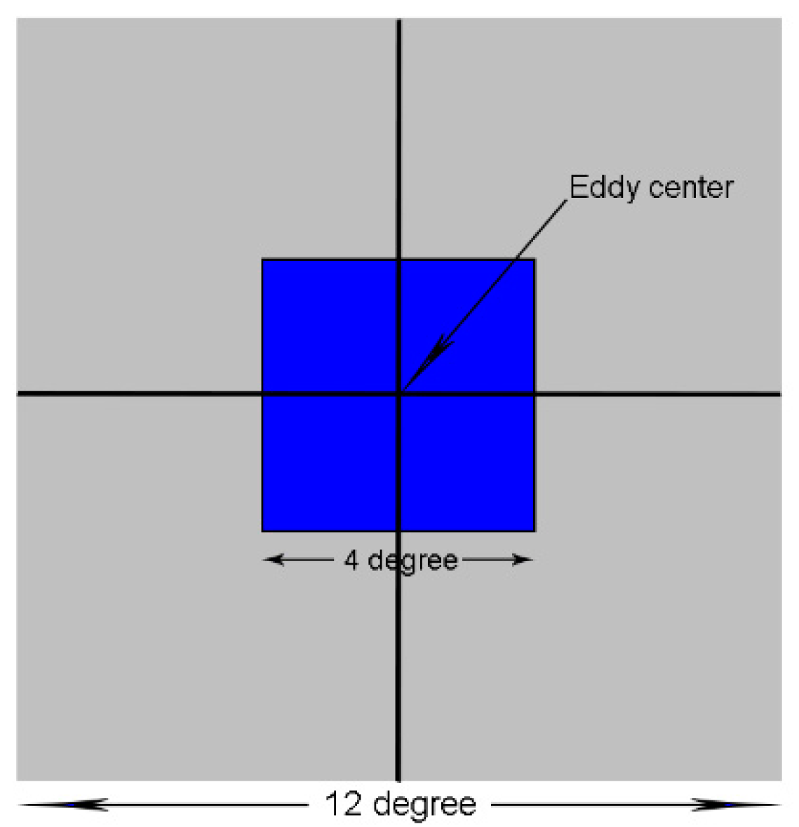
2.6. Method of Matching Atmospheric Variables with Oceanic Eddies

The fine-scale characteristics of atmospheric and oceanic variables (such as SST, wind speed and precipitation rate) are obtained through an 8° zonal moving average subtracted from each variable (the formula is X ( i , k ) = X ( i , k ) ( X ( i , k ) ) ¯ 8 ° z o n a l _ a v e r a g e , where X represents SST, precipitation rate, wind speed, etc.). Eddies with SSTA at the eddy center less than −0.05 °C (for cyclonic eddies) and larger than 0.05 °C (for anticyclonic eddies), and radii larger than 20 km, are selected. As a result, there are about 14,677, 19,636, 16,684 and 12,220 cyclonic eddies, and 14,469, 22,043, 16,747 and 13,195 anticyclonic eddies in the KE, SF, CC and AI regions, respectively. The matching method is adopted from Ma et al. [24]. Figure 1 is the schematic diagram for the matching method. The 4° × 4° bin is large enough to cover the oceanic eddy to undertake composite analysis. The bin 12° × 12° is selected as the background for the eddy field.

3. Results

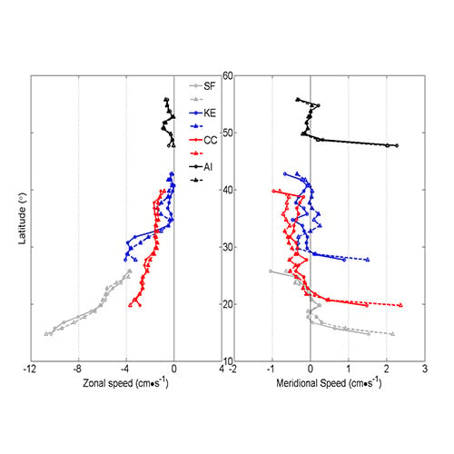
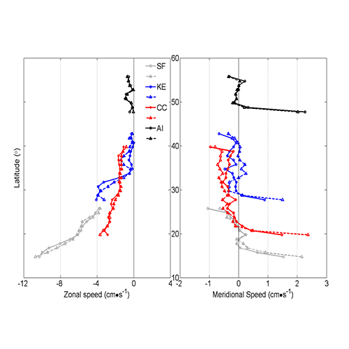
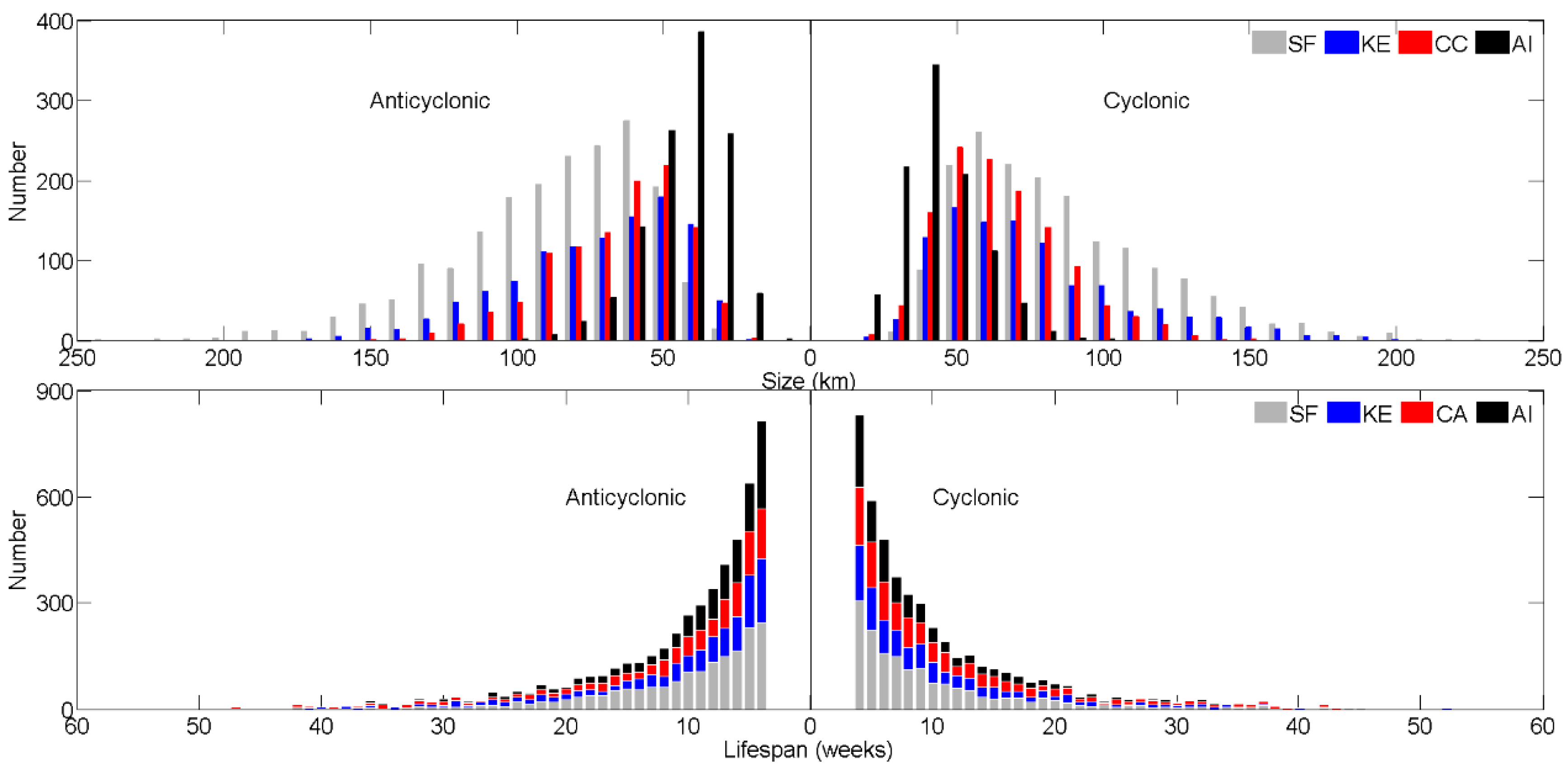
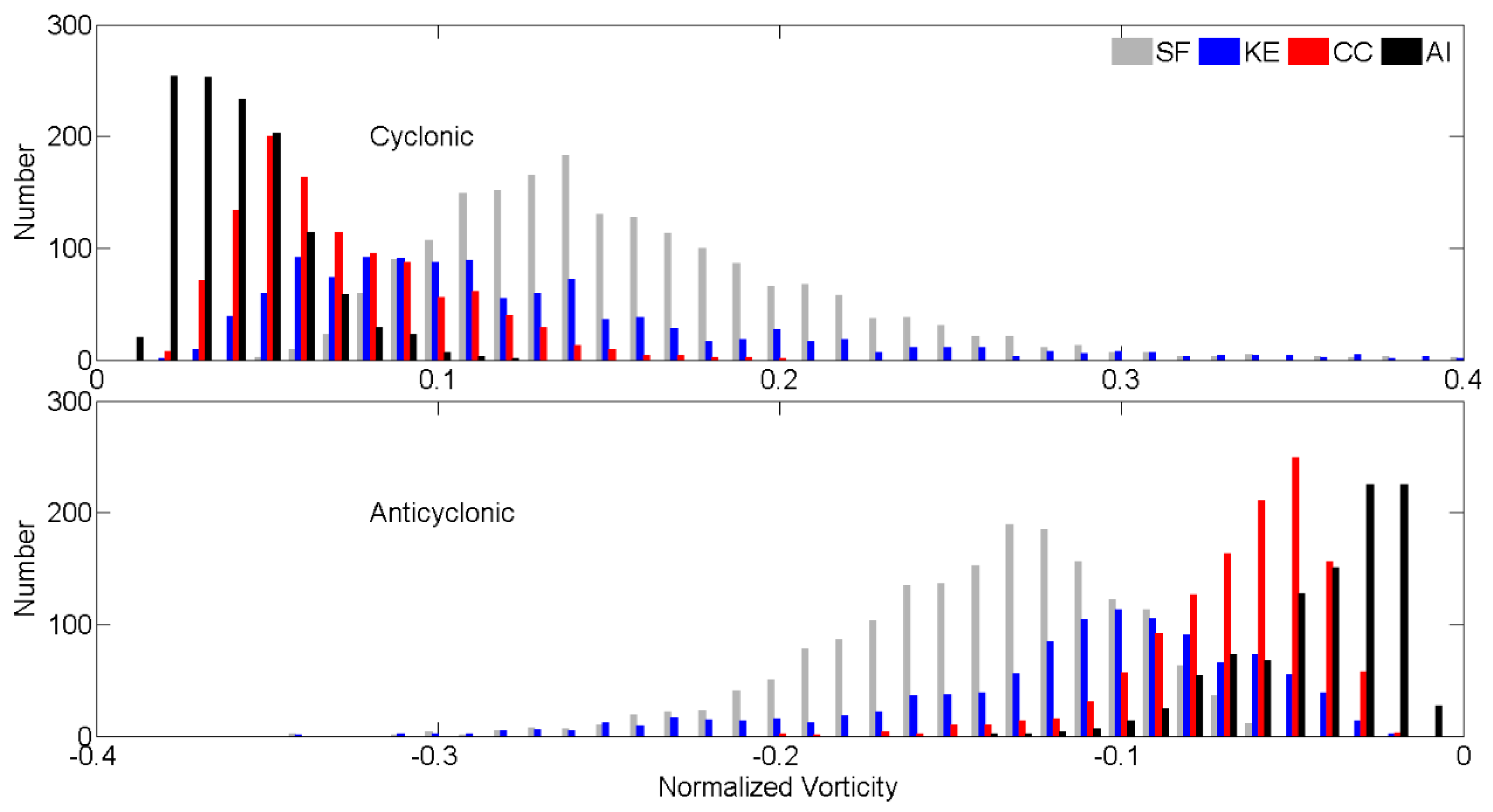
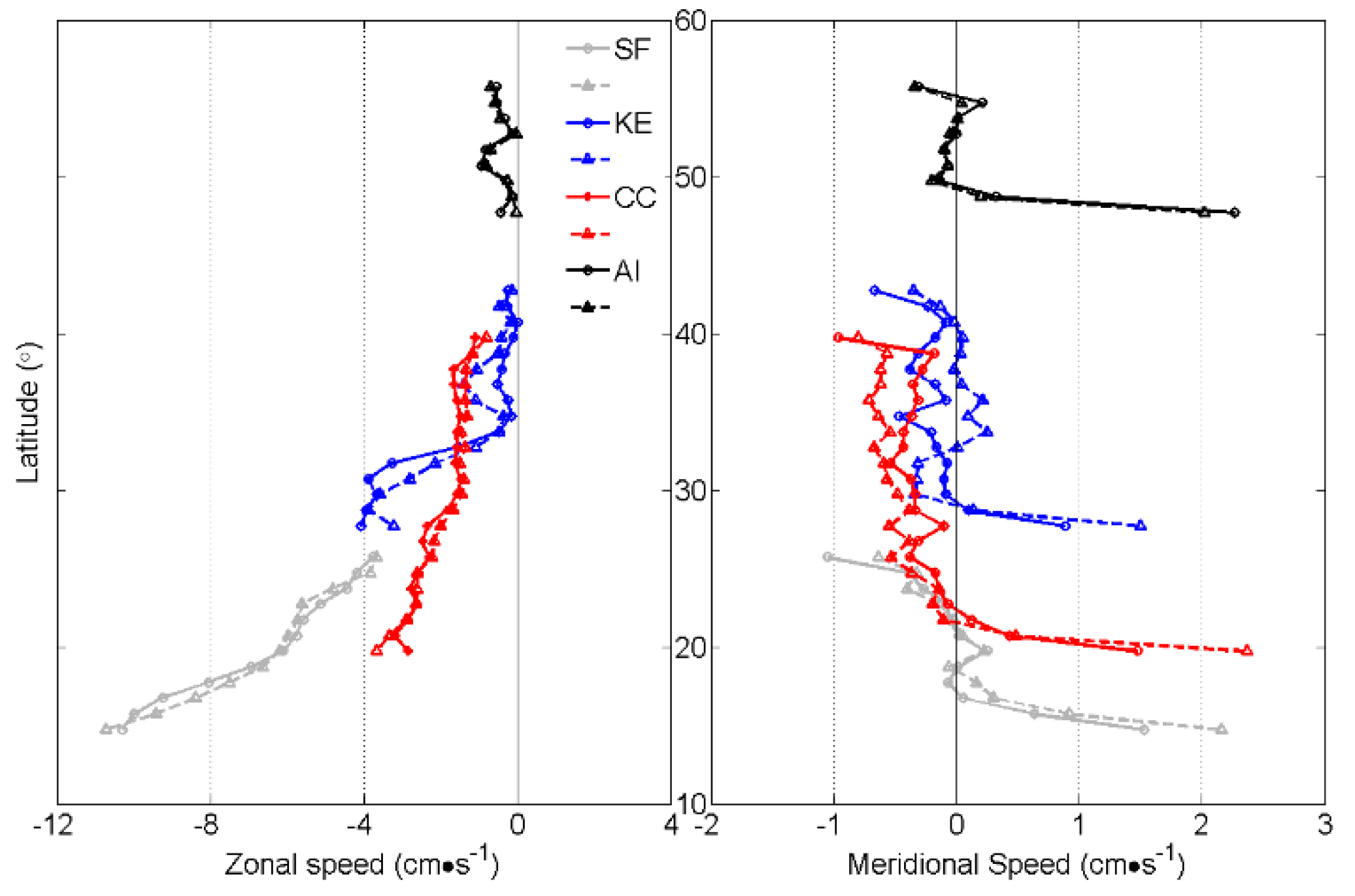
3.1. Statistics of Eddy Characteristics

Eddy kinetic energy (EKE) is used to characterize eddy activity intensities and is calculated by the formula: E K E = 1 2 ( u 2 + v 2 ) , where u′ and v′ are the geostrophic current anomalies. Figure 2 shows the 90-day high pass-filtered surface EKE averaged from 2002 to 2010 in the North Pacific. The highest EKE occurs in the KE and SF regions [42,43]. In addition, compared with adjacent areas, EKE is also high in the AI and CC regions. The largest EKE in the KE region is primarily caused by the strong horizontal shear and the meandering of the Kuroshio path [42]. The higher EKE in the SF region is predominantly modulated by the baroclinic instability of the background currents [44]. The CC region is characterized by strong eddy activity where the persistent equatorward wind causes coastal upwelling fronts. Instability of these upwelling fronts results in eddy generation. The instability of the coast shelf trapped jet causes the eddy formation in the AI region. One can see that the eddy generation mechanisms are varied in the four subdomains, which could cause a difference in mesoscale air–sea interaction characteristics in the four regions.
Satellite altimetry data provides an opportunity to characterize eddies in terms of their basic parameters such as polarity, lifetime, size, vorticity and moving speed in the four subdomains. We utilize two eddy counting methods. Eddy number is defined using the trajectory method (Lagrangian method: counting all the eddies over the course of its lifetime as one eddy [1]), and also through the snapshot method (Eulerian method: counting each individual eddy on the snapshot in each moment as one eddy [45]). Figure 3 shows the histogram of eddy radii and lifespans. The eddy size is the largest in the SF region and the smallest in the AI region (upper panels in Figure 3). Eddy sizes in the KE and CC regions are similar. The peak eddy radius differs in each subdomain, with 60–70 km in the SF region, about 50 km in the KE and CC regions, and only 40 km in the AI region. Eddy size decreases from the low to high latitudes. Eddy sizes at each latitude are close to the first baroclinic Rossby wave deformation radius [46], which mainly controls the eddy characteristics. According to Chelton et al. [46], when the latitude is greater than 5°, the first baroclinic Rossby wave deformation radius decreases poleward. Eddy lifespans are displayed on the bottom panels of Figure 3. Both cyclonic and anticyclonic eddy numbers decrease as lifespan increases. Eddies with lifespans equal to and longer than 4 weeks are selected for the present study, which reduces uncertainties in eddy detection.
Vorticity is one of the main parameters used to describe eddy intensity. Figure 4 presents the distributions of the eddy vorticity normalized by the local Coriolis coefficient for the four subdomains where it can be observed that the pattern follows a normal distribution. The eddy vorticity is defined at the approximate eddy center. The largest normalized eddy vorticity at the peak occurs in the SF domain (anticyclone: −0.13, cyclone: 0.14), the smallest in the AI region (anticyclone: −0.03, cyclone: 0.03). Normalized vorticity at the peak is about −0.1 (0.1) for anticyclonic (cyclonic) eddies in the KE region and −0.04 (0.04) in the CC region. The oceanic eddies are stronger in SF and KE due to the strong baroclinic instability in these two areas. In detail, in the SF and KE regions, the strong density front is presented around the year. Due to the baroclinic instability, the high available potential energy stored in the density front in the SF and KE regions is released to the eddy kinetic energy, causing strong eddy activities in these two regions.
Eddy movement is also an essential eddy characteristic. Westward movement is a common feature for the eddies in all four domains (left panel in Figure 5). In the SF area, the westward propagation speed is between 3.8–11.1 cm·s−1. Furthermore, the speed decreases with increasing latitude. The same distribution is observed in the CC region but with zonal speeds ranging from 0.8 to 3.93 cm·s−1. In the KE region, the westward movement increases with the latitude till 30°N, then decreases to almost zero at around 33°N. It increases between 33 and 36°N, and then decreases with the latitude. This behavior is because the main axis of the eastward KE current located near 35°N obstructs the westward movement of eddies. In the AI domain, the eddies propagate westward with a small zonal speed in a range of 0 to 0.93 cm·s−1. These results are generally congruent with results observed by Chelton et al. [46], which show that eddy propagation speed is of the same order as the first baroclinic Rossby wave propagation speed decreasing with the latitude. The curves of the northward movements of eddies in the four subdomains share a similar "Z-shape" (right panel of Figure 5). Eddies in the southern part of each subdomain tend to move northward with larger speeds, while eddies in the northern part move southward with smaller speeds.

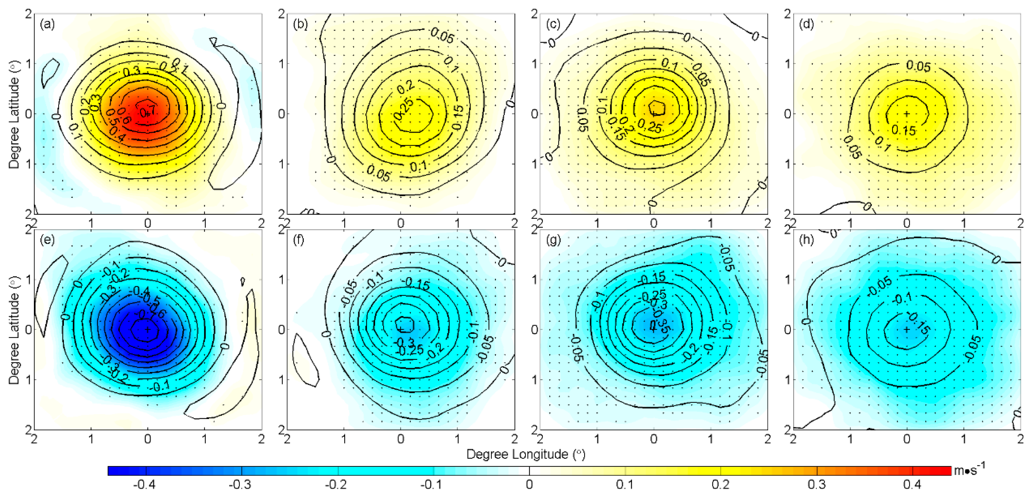
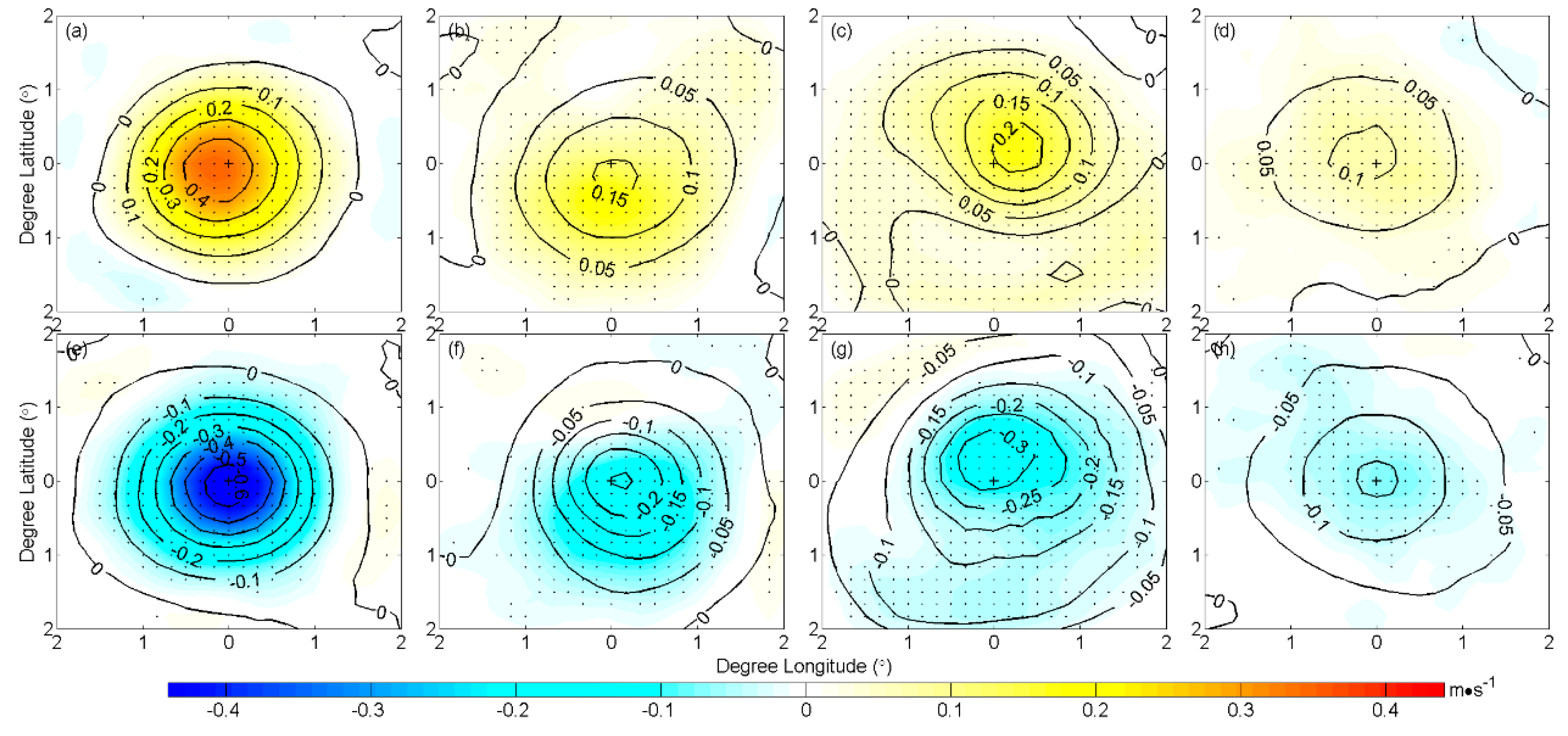
3.2. Atmospheric Responses to Eddies
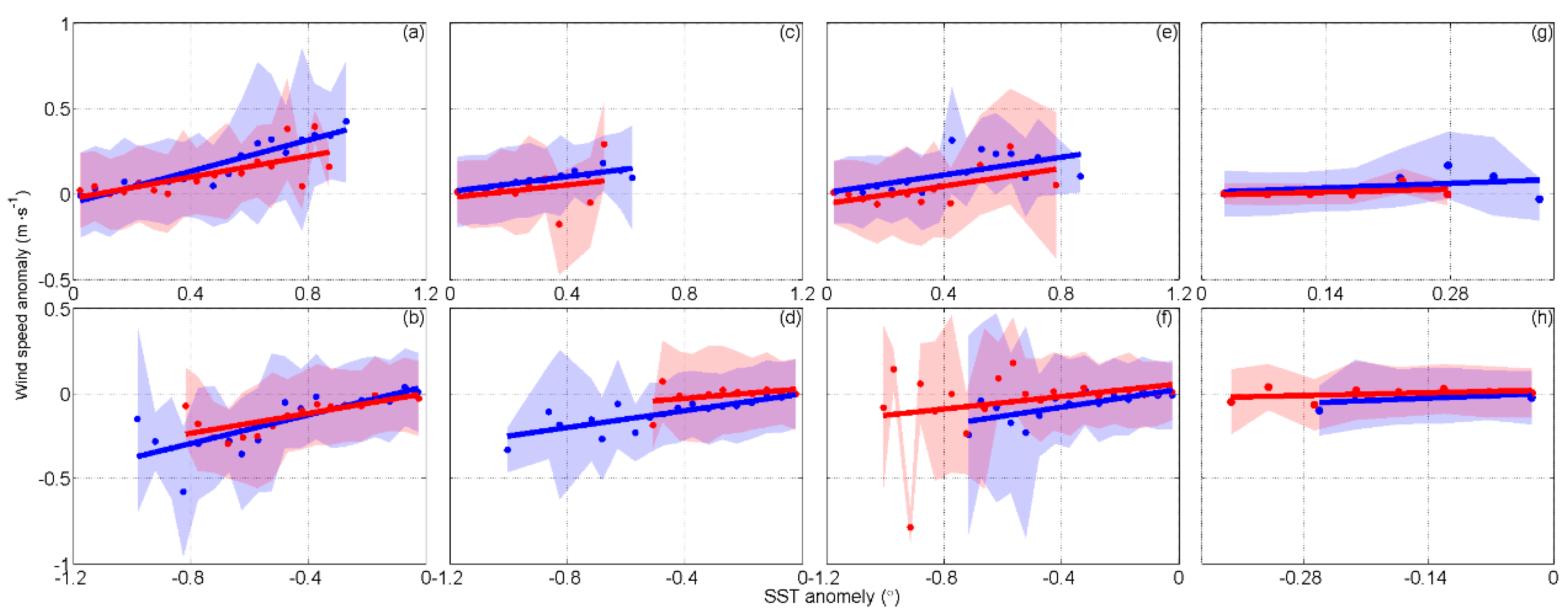
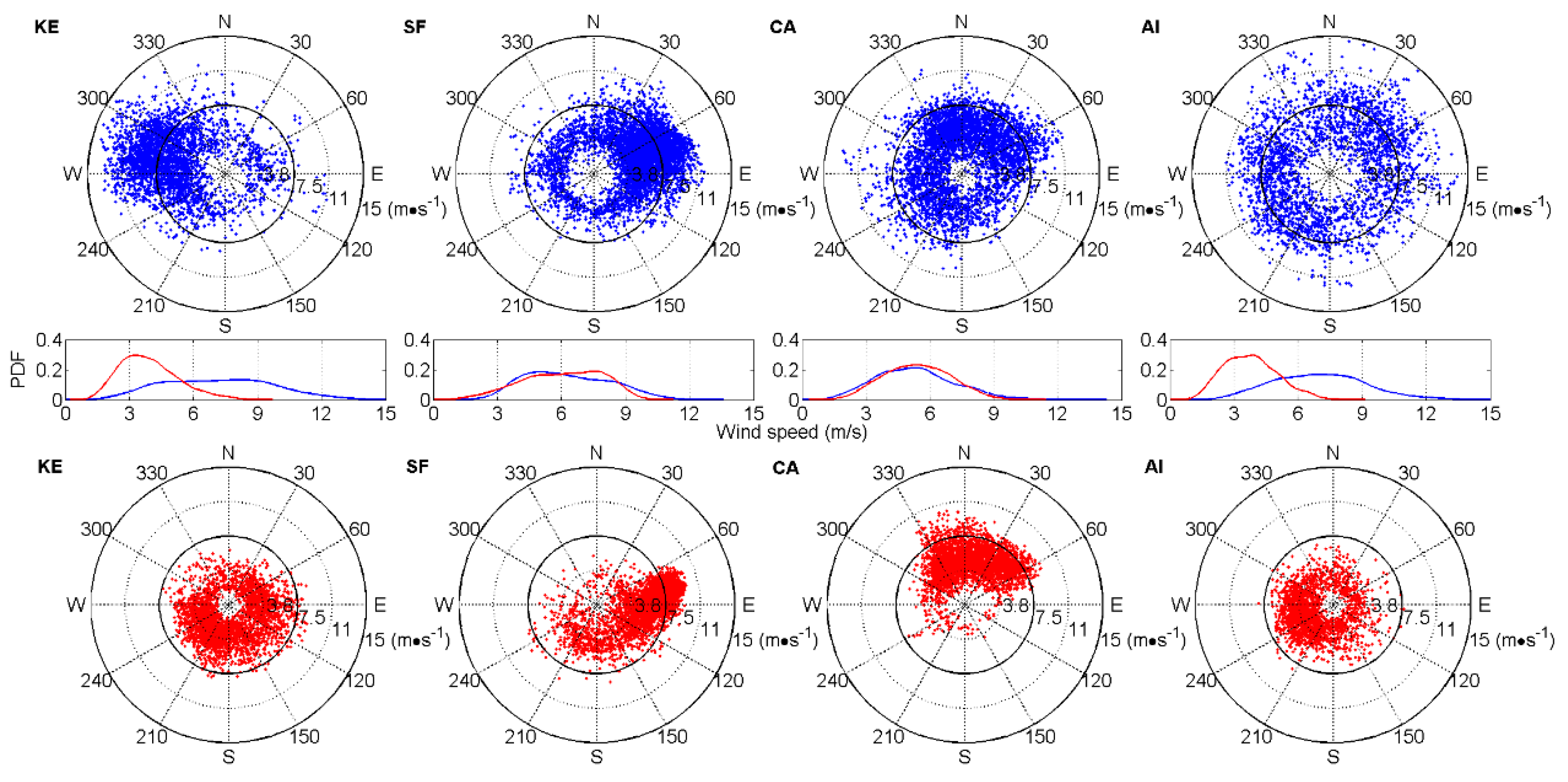
3.2.1. Wind Speed

Atmospheric responses to oceanic mesoscale eddies are primarily manifested in sea surface winds, precipitation and heat fluxes. Figure 6 and Figure 7, respectively, show the winter and summer composites of SST and sea surface wind speed anomalies in response to the oceanic eddies. In each subdomain, wind speed anomalies are positive for anticyclonic eddies both in winter and summer, and negative for cyclonic eddies. Furthermore, the maximum wind speed anomalies are located over the eddy center, corresponding to the maximum SST anomalies. However, the magnitudes of the wind speed anomalies vary from region to region and exhibit a distinct seasonal variability. During the wintertime, the wind speed anomaly and SSTA is the strongest in the KE region (0.5 m·s−1, 0.7 °C). However, little difference can be observed in the other three subdomains (0.2–0.3 m·s−1, 0.15–0.3 °C). In summer, wind speed anomaly and SSTA is still the largest in the KE region (0.35 m·s−1, 0.7 °C) and the smallest in the AI region (0.1 m·s−1). The wind speed anomaly (SSTA) is about 0.2 m·s−1 (0.25 °C) in both SF and CC regions. Therefore, regardless of season, the eddy impacts on the sea surface wind speed and sea surface temperature are the strongest in the KE region.

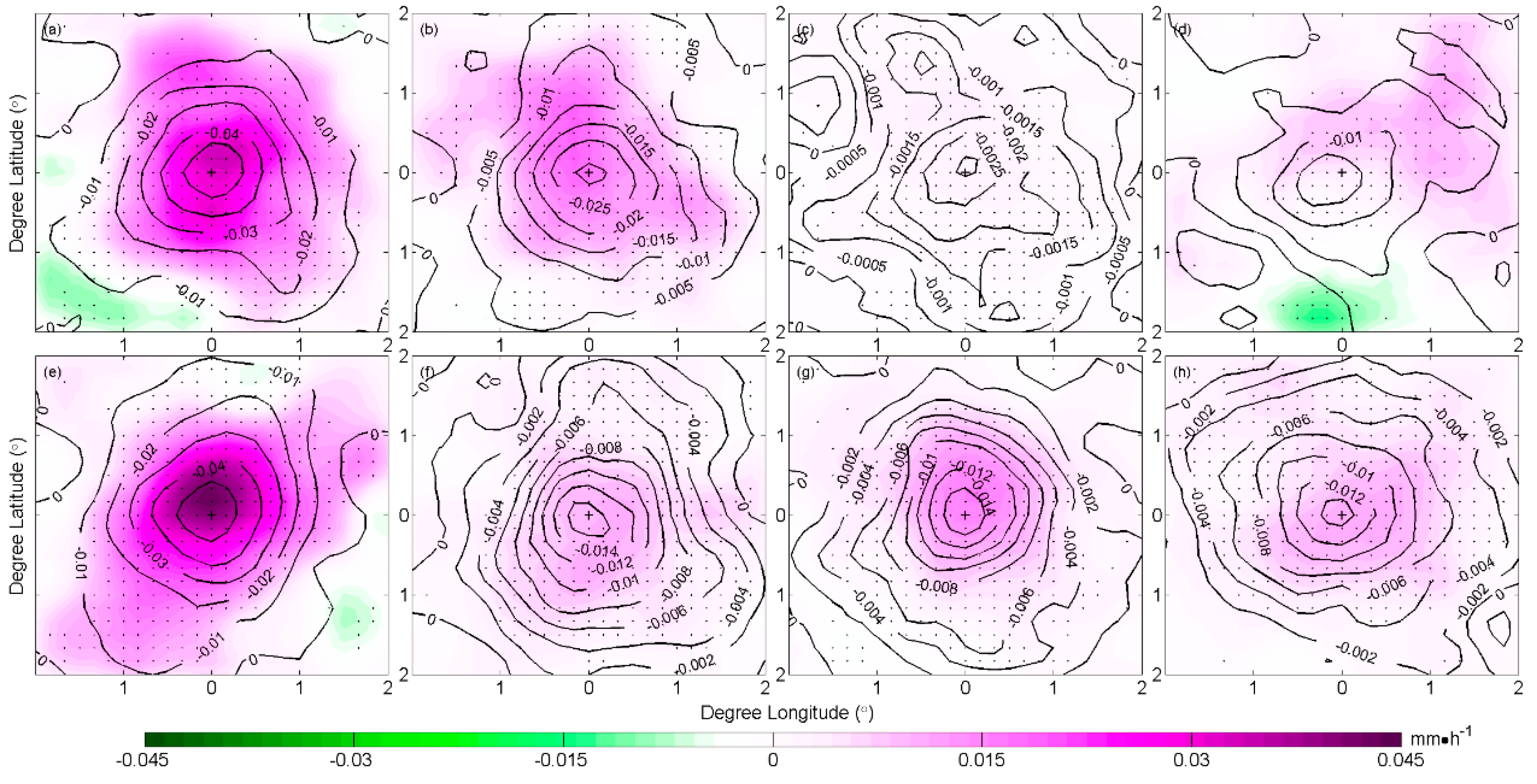
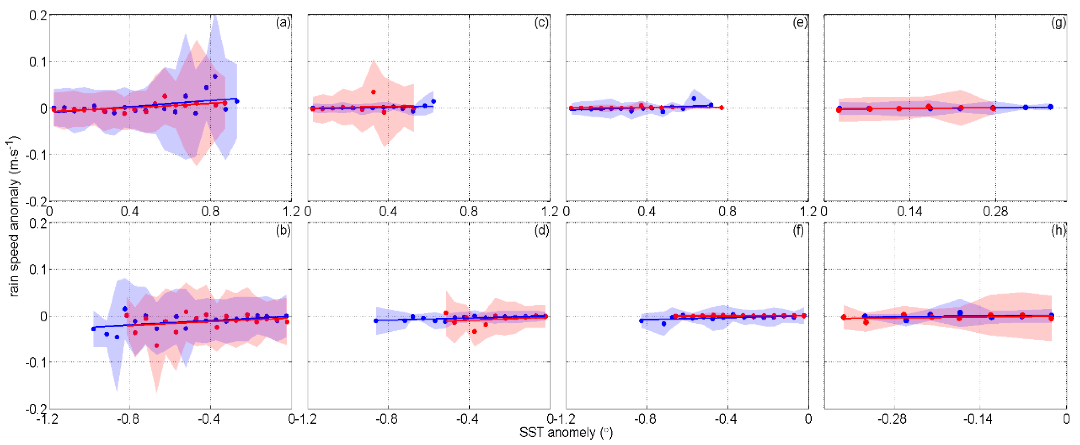
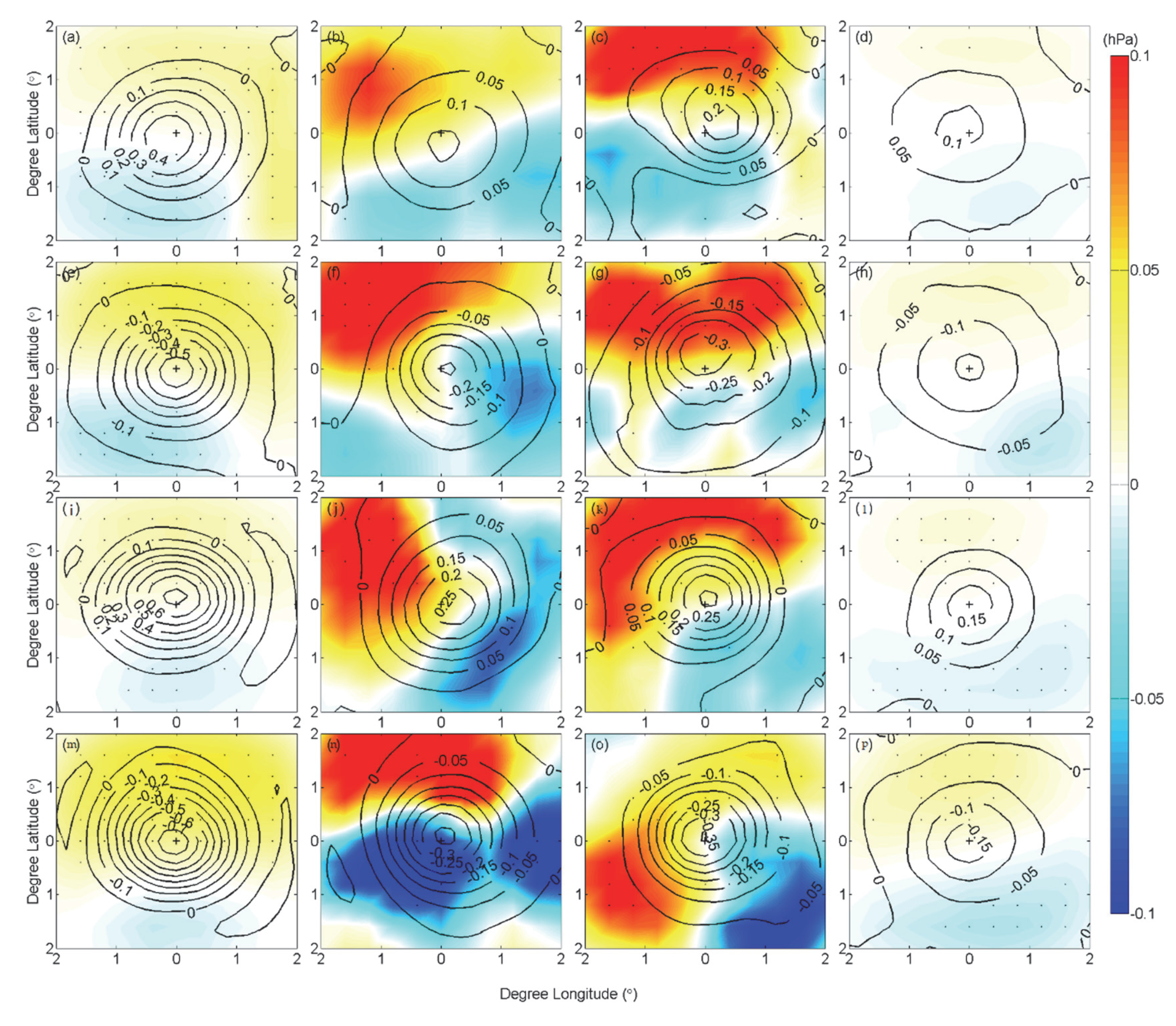
3.2.2. Precipitation
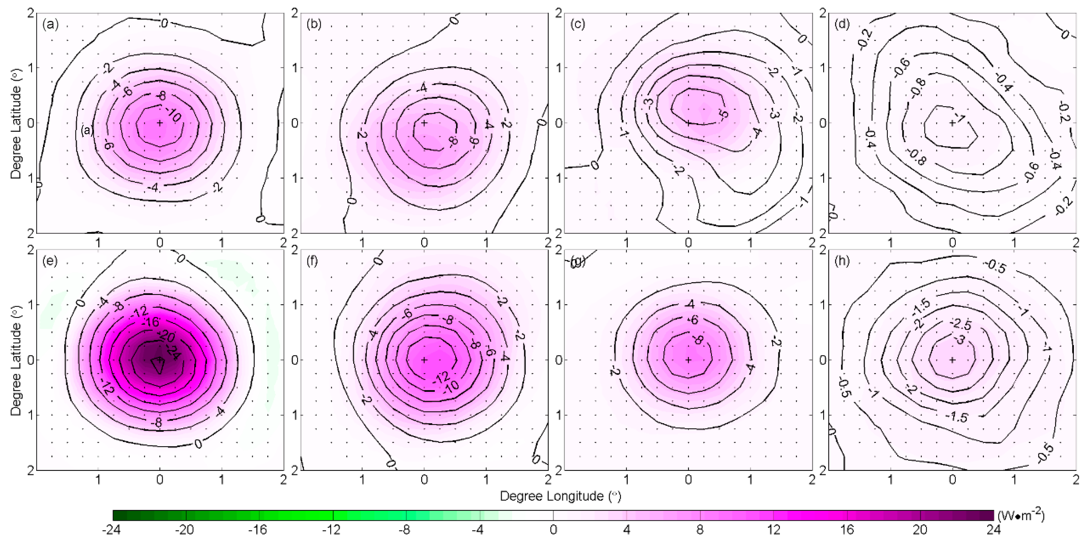
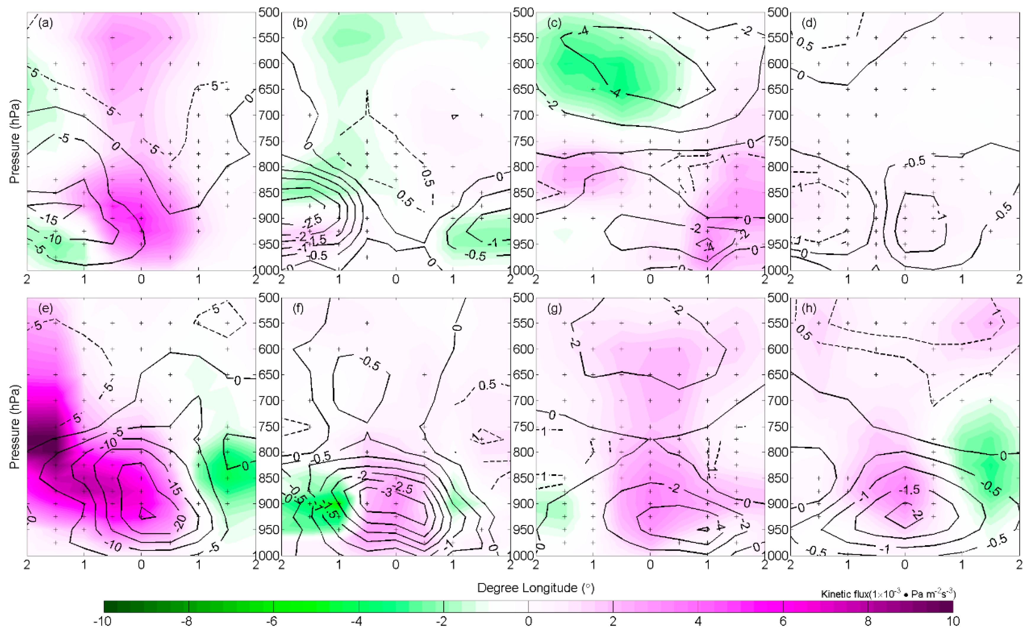
As shown by the previous analyses, oceanic eddies thus contribute to SST and wind speed anomalies. Moreover, mesoscale eddies also influence the local cloud coverage and precipitation due to changes in atmospheric stability and anomalous secondary circulation. Previous studies [6,28] show that this can happen in two ways: vertical motion caused by anomalous surface divergence (dynamic effect), and changes in the water vapor content (thermodynamic effect).
Figure 8 displays composites of precipitation above oceanic eddies. The precipitationrate anomaly above anticyclonic eddies is positive (negative in cyclonic eddies) in agreement with previous studies [24,28]. However, the magnitudes of the precipitation rate anomalies differed among the subdomains. In winter, the largest and smallest anomalies occur in the KE and AI regions, respectively. The CC and SF regions follow after the KE region. Summer and winter present distinct, regional dependence of precipitation. The maximum value is still located in the KE region while the minimum value appears in the CC region, instead of the AI area. In addition, in comparison with the winter season, the magnitude of the precipitation rate anomaly increases in the SF region, in contrast to the wind speed anomaly displayed in Figure 6 and Figure 7. This observation may be related to the difference in the atmospheric environment of each subdomain. More detailed discussions are given in Section 4.

3.2.3. Heat Flux

Latent and sensible heat fluxes are two crucial factors in the transfer of heat between the ocean and atmosphere. When an air mass moves over a mesoscale eddy, a turbulent heat flux anomaly is caused by differences in humidity in addition to SST and wind speed anomalies at the ocean surface. For anticyclonic eddies, warm SST anomalies increase the temperature difference between the ocean and atmosphere, and increase the sensible heat flux transfer from the ocean to the atmosphere. Simultaneously, the anomalous warming also increases the saturated specific humidity, which in turn increases the humidity difference between sea and air. Thus, the evaporative cooling at the sea surface is enhanced and the latent heat flux increases. Therefore, anticyclonic eddies correspond to upward turbulent heat flux anomalies; that is, the ocean heats the atmosphere. On the other hand, cyclonic eddies correspond to downward turbulent heat flux anomalies, where the ocean absorbs heat from the atmosphere [24].
The contours in Figure 9 show that negative latent heat flux anomalies are indeed found above cyclonic eddies in winter and summer (sensible heat flux anomalies are not shown since they have the same pattern). The shading in Figure 9 shows the opposite case of an anticyclonic anomaly. Table 1 shows the maximum sensible and latent heat flux anomalies, enhanced by the oceanic mesoscale eddies in the KE, SF, CC and AI regions. The heat flux altered by oceanic mesoscale eddies is stronger in winter than summer. The atmospheric response to SST anomalies of oceanic mesoscale eddies is the strongest in the KE region and the weakest in the AI region. Here, the influence of eddies on heat flux is slightly stronger in cyclonic than anticyclonic eddies.

4. Possible Mechanisms for Atmospheric Response and Regional Dependence

To investigate the regional dependence of the atmospheric response to oceanic mesoscale eddies in the four eddy activity regions, we quantify the change of various properties with the SST anomaly. There is a high correlation between atmospheric parameters (wind speed, precipitation rate) and SSTA (correlation coefficients are not shown here). The regression of SSTA and wind speed (precipitation rate) anomaly in the four subdomains and seasons are investigated in Figure 10 and Figure 11. In addition, Table 2 summarizes the linear regression coefficients of wind speed and precipitation rate anomalies onto SST anomalies for cyclonic and anticyclonic eddies in each subdomain during winter and summer. The response of wind speed to oceanic mesoscale eddies is much stronger during winter in the four subdomains than during summer. However, regardless of the subdomain, the wind speed anomaly above the cyclonic eddies is slightly stronger than that above anticyclonic eddies. Comparing the response of wind speed to SST in all four subdomains, the strongest response occurs in the KE region, followed by CC and SF domains, and the weakest is in the AI region.
Due to the limited observational data, a CFSR reanalysis dataset is used to provide atmospheric variables both at the surface and in the vertical levels, which allow us to further investigate the mechanism underlying atmosphere responses to oceanic eddies. Although not shown, composites of SST, wind speed, precipitation and heat flux anomalies from the reanalysis data show similar patterns, but the magnitude is slightly smaller than that of observed data. Furthermore, the SST anomaly has a good linear relationship with other variables (wind speed, precipitation rate, sensible heat flux and latent heat flux). The maximum SST anomaly corresponds to the largest wind speed, precipitation rate, sensible heat flux and latent heat flux anomalies. Previous studies show that the wind speed weakens or strengthens above oceanic eddies depending on the strength of atmospheric vertical kinetic energy flux [24,47]. In this study, we propose three parameters which could influence the vertical energy transport: (1) intensity of SST anomalies (or eddy size), (2) stability of atmospheric stratification (potential temperature shown in Figure 13), and (3) vertical mixing term (the transient kinetic energy flux shown in Figure 14).
The main factor which increases or decreases the wind speed happens through SST anomalies due to heat fluxes across the air–sea interface. The eddy size controls the area that can be influenced by SST anomalies. Sun et al. [48] suggest two main impacts of SST-wind speed coupling: the SST gradient associate with mesoscale progresses and wind speed steadiness. For detectable mesoscale coupling to occur, they determine that a constant wind speed plays a crucial role, especially when the SST gradients associated with mesoscale progresses are relatively weak. Chelton et al. [49] find that variations in the wind directional steadiness mainly modulate mesoscale SST-wind coupling. It should be noted that the SST anomaly in this study is defined as a spatial anomaly with respect to the SST in the surrounding area. The SST anomaly inside an eddy is equivalent to the SST gradient, except that it is divided by the eddy radius. Therefore, one can consider that the relationship between the wind speed anomaly and SST anomaly inside an eddy is equivalent to the wind speed anomaly and SST gradient, as discussed by Sun et al. [48] and Chelton et al. [49]. As the Kuroshio region carries the warm water far from the equator, the water temperature contrast in KE to the adjusting area is large, so the eddies shed off the Kuroshio region are highly energetic, which makes the SST anomaly in the KE area is the largest among the four selected areas. As Figure 6 and Figure 7 show, SST anomalies are noticeably larger in the winter regardless of the domain, and the SSTA maximum occurs in the KE region, followed by the CC and SF area, and the smallest in the AI subdomain. Furthermore, Figure 12 illustrates the rose scatter distribution and the Probability Distribution Function (PDF) of wind speed in the four areas in summer and winter. By comparing the magnitude of wind speed in winter and summer, it is noted that the wind is stronger in winter than in summer in all subdomains. The PDF of wind speed in the KE and AI regions shows a similar distribution both with a peak value of 3–4 m·s−1. However, the wind speed anomalies in the KE region are stronger than in the AI area (Figure 6 and Figure 7).
Wallace et al. [33] proposed that variability in atmospheric stability could influence vertical momentum transport, and hence the sea surface wind. The vertical profile of potential temperature is used to represent the stability of the MABL. Figure 13 displays the composited vertical profiles of potential temperature over the eddy centers in winter and summer. Steeper slopes correspond to weaker stratifications (stronger instability), indicating that kinetic energy can be transported to the sea surface, ultimately leading to larger wind speed anomalies. In the KE region, potential temperature changes little with an altitude below 900 hPa in winter, indicating that the atmosphere is relatively unstable. By contrast, potential temperature decreases with altitude in summer, suggestive of a stable atmosphere. Similarly, the slope of potential temperature profile under 900 hPa in the SF region is steeper in winter than summer. In the CC and AI regions, the potential temperature increases quickly above 950 hPa in summer, rather than during the winter. The difference in atmospheric stability between winter and summer may be the primary cause of the seasonal dependence of atmospheric responses in the KE region. Among the four subdomains, the slope of potential temperature profile below 900 hPa is steepest in the KE domain, followed by the SF, AI and CC regions, indicative of the strongest instability in the KE region. This observation is potentially linked to the strongest surface wind speed response in the KE region.
The transitional kinetic energy (TKE) flux ω ( u 2 + v 2 ) ¯ is an important parameter which is used to represent how ocean eddies affect the above atmosphere through the vertical mixing mechanism, where ω , u and v are synoptic scale transient vertical, zonal and meridional wind velocities at isobaric levels. If ω ( u 2 + v 2 ) ¯ is positive (negative), the transitional energy is transported downward toward (upward and away from) the sea surface, thus increasing (decreasing) the wind speed at the sea surface. Figure 14 shows the longitude-height cross-section of composite ω ( u 2 + v 2 ) ¯ along the eddy center. From Figure 14, it can be seen that ω ( u 2 + v 2 ) ¯ is almost positive for anticyclonic eddies, showing downward energy transport; the opposite is true of cyclonic eddies. Further, the maximum TKE flux is located in the KE region regardless of the season, followed by the SF and the CC regions, and the weakest in the AI area. It is consistent with the wind speed anomalies shown in Figure 6 and Figure 7. In addition, the maximum TKE flux for anticyclonic eddies is observed above 800 hPa and almost reaches 900 hPa in the SF, CC and AI regions. The TKE flux in the AI region is the weakest among the four subdomains. Moreover, the maximum TKE flux of the cyclonic eddies is slightly larger than that of the anticyclonic eddies. Furthermore, the TKE flux is weaker during summer than in winter in all four subdomains. It corresponds to larger wind speed anomaly in winter than in summer (Table 2).
The SLP adjustment mechanism was first suggested by Lindzen et al. 1978 [21], which requires that negative pressure anomaly occurs over the anticyclonic eddy, and positive pressure anomaly occurs over the cyclonic eddy. Figure 15 shows the composites of SLP anomaly over anticyclonic and cyclonic eddies in the four areas. The SLP anomalies are characterized by dipole patterns, different from what is expected from the SLP adjustment mechanism. Therefore, we conclude that the SLP adjustment is not a dominant mechanism for the atmospheric responses to the oceanic eddies in these four regions.
The seasonal difference in precipitation rate anomalies to 1 °C of SSTA differs among the four subdomains, with stronger responses in winter over the KE, CC and AI regions, but a larger response in summer over the SF region (Figure 8). These results may be related to the seasonal variations in precipitation over these regions. In the SF region, more precipitation occurs in summer due to the influence of the summer monsoon. Wang et al. [50] showed that the SF region is one of the peak rainfall regions during the Asia–Pacific summer monsoon. In the midlatitudes, the majority of winter precipitation is associated with frontal systems and related cyclonic activities. In the KE region, the extratropical storms may be the primary contributor to heavy precipitation in winter [51]. The Aleutian Low (AL) is one of the principal causal factors of both the synoptic and climatic conditions in the AI region. In addition, the AL is a deep baroclinic atmospheric system with a low-pressure center that can almost reach the surface. That is why the wind direction in the AI region displays a circular pattern (Figure 12). The CC region is influenced by a tropical Mediterranean-type climate characterized by wet winters and dry summers [52]. The westerly wind path is located closer to the tropical area in winter than in summer, which means that the path of the extratropical cyclone through California could bring more vapor through the atmospheric river. Winter storm tracks and extratropical cyclones heavily influence rainfall in the CC region. In the summer, northeasterly wind prevails (upper panel in Figure 12), carrying less humidity as east of California is a desert area and induces upwelling along the coast. Cold bottom water is brought up to the surface, thus cooling the air above the current and reducing evaporation.

5. Conclusions and Discussion

In this study, we chose four eddy rich regions, which are separated from each other by over 1000 km geographically, so there is no mutual relationship between them and they do not affect each other. Based on the above discussion, one can clearly see that there are common influencing factors and also differences in the atmospheric responses to the oceanic eddies among these four areas. The common parts can be summarized as: The increase in the SSTA can cause increases in the sea surface wind, precipitation rate and heat flux, and vice versa. The underlying mechanism driving the atmosphere responses is the vertical kinetic energy flux among the four areas. The different parts can be summarized as: The atmospheric responses (wind speed, precipitation rate) are the strongest and weakest in the KE and AI (or CC) regions. The strong seasonal variation difference in the atmospheric responses are presented. As any type of observational and reanalysis product, uncertainties exist in the data we use in the present study. Based on the validations by the producer of these products, the level of uncertainty is acceptable for the scientific studies. Therefore, these uncertainties associated with the data used do not change the conclusion reached by the present study.
Through the above investigation, the EKE, eddy characteristic, SSTA and atmospheric stability vary across the four subdomains and seasons, and could be responsible for differences in mesoscale air–sea interaction characteristics. In addition, several meteorological quantities (SST, wind speed, precipitation, potential temperature, and the heat and TKE fluxes) are statistically examined and a dynamic analysis is performed. It is observed that anticyclonic eddies lead to an enhancement of SST, surface wind speed, precipitation and heat flux over the eddy center, while cyclonic eddies show the opposite.
By comparing composites for the SST, wind speed and heat flux anomalies in the four subdomains, the strongest response is always observed in the KE region, followed by the CC and the SF regions, and the AI region shows the weakest response. However, it is slightly different for precipitation anomalies over the oceanic eddies. The observations might be related to the different magnitude of seasonal precipitation over the four subdomains. The strongest responses are found in the KE, CC and AI in winter. However, in summer it is worth noting that the weakest response shows in the CC region instead of the AI region like the other variables mentioned above, and the strongest response is still observed in the KE area. In addition, the precipitation in the SF region is contrary to the other three subdomains: the strongest response shows in summer with the influence of the summer monsoon acting as the background of the atmosphere.
The same method is applied to the CFSR product. Similar variations for each variable occur in the four subdomains. It also shows that surface wind speed responses to oceanic eddies are stronger in winter than in summer, which can be partially explained by the potential temperature profile and the TKE flux ω ( u 2 + v 2 ) ¯ anomalies. The slope of the potential temperature profile below 900 hPa is steepest in the KE domain, followed by the SF, AI, and CC regions, indicative of the strongest instability in the KE region, which is related to the strongest surface wind speed. The TKE flux is positive above anticyclonic eddies, indicating that energy transport is downward as sea surface wind speed increases; the opposite is true for cyclonic eddies. Through the analysis of SSTA, potential temperature and the TKE flux, it was found that there exists a regional dependence of the atmospheric responses to oceanic eddies.

Author Contributions

All authors have read and agree to the published version of the manuscript. Conceptualization, J.J. and C.D.; methodology, J.M. and J.J.; software, J.J.; validation, J.C.H.C., D.C. and M.J.; formal analysis, J.J.; investigation, J.J.; resources, D.C.; data curation, J.J.; writing—original draft preparation, J.J.; writing—review and editing, J.C.H.C., J.M., C.D., and D.C.; visualization, J.J.; supervision, D.C.; project administration, C.D.; funding acquisition, D.C. and C.D.

Funding

This research is funded by the National Key Research and Development Program of China (2017YFA0604100), National Programme on Global Change and Air–Sea Interaction (GASI-IPOVAI-04), the National Key Research and Development Program of China (2016YFA0601803 and 2016YFC1401407),the National Natural Science Foundation of China (41476022, 41490643, 41730535 and 41706008), the Startup Foundation for Introducing Talent of Nanjing University of Information Science & Technology (2014r072), the Program for Innovation Research and Entrepreneurship team in Jiangsu Province (2191061503801), the National Programme on Global Change and Air–Sea Interaction (GASI-IPOVAI-02, GASI-03-IPOVAI-05), the National Science Foundation of China (OCE 06-23011) and the China Ocean Mineral Resources R & D Association (DY135-E2-2-02, DY135-E2-3-01).

Acknowledgments

The authors would like to thank Yu Liu for his early stage work. Thanks are also extended to Kenny T.C. Lim Kam Sian for improving the writing. The altimeter products were produced and distributed by Aviso+ (https://www.aviso.altimetry.fr/), as part of the Ssalto ground processing segment. AMSR data are produced by Remote Sensing Systems and were sponsored by the NASA AMSR-E Science Team and the NASA Earth Science MEaSUREs Program. The Japanese ocean flux data set using remote-sensing observations J-OFURO (http://dtsv.scc.u-tokai.ac.jp/j-ofuro/).

Conflicts of Interest

The authors declare no conflict of interest.

References

  1. Chelton, D.B.; Schlax, M.G.; Samelson, R.M. Global observations of nonlinear mesoscale eddies. Prog. Oceanogr. 2011, 91, 167–216. [Google Scholar] [CrossRef]
  2. Chelton, D. Ocean–atmosphere coupling: Mesoscale eddy effects. Nat. Geosci. 2013, 6, 594. [Google Scholar] [CrossRef]
  3. Zhang, Z.; Zhong, Y.; Tian, J.; Yang, Q.; Zhao, W. Estimation of eddy heat transport in the global ocean from Argo data. Acta Oceanol. Sin. 2014, 33, 42–47. [Google Scholar] [CrossRef]
  4. Faghmous, J.H.; Frenger, I.; Yao, Y.; Warmka, R.; Lindell, A.; Kumar, V. A daily global mesoscale ocean eddy dataset from satellite altimetry. Sci. Data 2015, 2, 150028. [Google Scholar] [CrossRef] [PubMed] [Green Version]
  5. Luecke, C.A.; Arbic, B.K.; Bassette, S.L.; Richman, J.G.; Shriver, J.F.; Alford, M.H.; Smedstad, O.M.; Timko, P.G.; Trossman, D.S.; Wallcraft, A.J. The global mesoscale eddy available potential energy field in models and observations. J. Geophys. Res. Ocean. 2017, 122, 9126–9143. [Google Scholar] [CrossRef]
  6. Chen, G.; Han, G. Contrasting Short-Lived With Long-Lived Mesoscale Eddies in the Global Ocean. J. Geophys. Res. Ocean. 2019, 124, 3149–3167. [Google Scholar] [CrossRef]
  7. Roemmich, D.; Gilson, J. Eddy transport of heat and thermocline waters in the North Pacific: A key to interannual/decadal climate variability? J. Phys. Oceanogr. 2001, 31, 675–687. [Google Scholar] [CrossRef]
  8. Chelton, D.B.; Schlax, M.G.; Samelson, R.M.; de Szoeke, R.A. Global observations of large oceanic eddies. Geophys. Res. Lett. 2007, 34, L15606. [Google Scholar] [CrossRef]
  9. Chelton, D.B.; Xie, S.P. Coupled ocean-atmosphere interaction at oceanic mesoscales. Oceanography 2010, 23, 52–69. [Google Scholar] [CrossRef]
  10. Volkov, D.L.; Lee, T.; Fu, L.L. Eddy-induced meridional heat transport in the ocean. Geophys. Res. Lett. 2008, 35, L20601. [Google Scholar] [CrossRef] [Green Version]
  11. Wang, X.; Li, W.; Qi, Y.; Han, G. Heat, salt and volume transports by eddies in the vicinity of the Luzon Strait. Deep Sea Res. Part I Oceanogr. Res. Papers 2012, 61, 21–33. [Google Scholar] [CrossRef]
  12. Bishop, S.P.; Watts, D.R.; Donohue, K.A. Divergent eddy heat fluxes in the Kuroshio extension at 144–148 E. Part I: Mean structure. J. Phys. Oceanogr. 2013, 43, 1533–1550. [Google Scholar] [CrossRef] [Green Version]
  13. Dong, C.; McWilliams, J.C.; Liu, Y.; Chen, D. Global heat and salt transports by eddy movement. Nat. Commun. 2014, 5, 3294. [Google Scholar] [CrossRef] [PubMed] [Green Version]
  14. Zhang, Z.; Wang, W.; Qiu, B. Oceanic mass transport by mesoscale eddies. Science 2014, 345, 322–324. [Google Scholar] [CrossRef] [PubMed]
  15. Griffies, S.M.; Winton, M.; Anderson, W.G.; Benson, R.; Delworth, T.L.; Dufour, C.O.; Dunne, J.P.; Goddard, P.; Morrison, A.K.; Rosati, A.; et al. Impacts on ocean heat from transient mesoscale eddies in a hierarchy of climate models. J. Clim. 2015, 28, 952–977. [Google Scholar] [CrossRef]
  16. Guo, M.; Xiu, P.; Li, S.; Chai, F.; Xue, H.; Zhou, K.; Dai, M. Seasonal variability and mechanisms regulating chlorophyll distribution in mesoscale eddies in the South China Sea. J. Geophys. Res. Ocean. 2017, 122, 5329–5347. [Google Scholar] [CrossRef]
  17. Doddridge, E.W.; Marshall, D.P. Implications of Eddy Cancellation for Nutrient Distribution within Subtropical Gyres. J. Geophys. Res. Ocean. 2018, 123, 6720–6735. [Google Scholar] [CrossRef]
  18. Huang, J.; Xu, F. Observational Evidence of Subsurface Chlorophyll Response to Mesoscale Eddies in the North Pacific. Geophys. Res. Lett. 2018, 45, 8462–8470. [Google Scholar] [CrossRef] [Green Version]
  19. Harrison, C.S.; Long, M.C.; Lovenduski, N.S.; Moore, J.K. Mesoscale effects on carbon export: A global perspective. Glob. Biogeochem. Cycles 2018, 32, 680–703. [Google Scholar] [CrossRef]
  20. Sun, B.; Liu, C.; Wang, F. Global meridional eddy heat transport inferred from Argo and altimetry observations. Sci. Rep. 2019, 9, 1345. [Google Scholar] [CrossRef] [Green Version]
  21. Minobe, S.; Kuwano-Yoshida, A.; Komori, N.; Xie, S.P.; Small, R.J. Influence of the Gulf Stream on the troposphere. Nature 2008, 452, 206. [Google Scholar] [CrossRef] [PubMed]
  22. Shimada, T.; Minobe, S. Global analysis of the pressure adjustment mechanism over sea surface temperature fronts using AIRS/Aqua data. Geophys. Res. Lett. 2011, 38, L06704. [Google Scholar] [CrossRef] [Green Version]
  23. Byrne, D.; Münnich, M.; Frenger, I.; Gruber, N. Mesoscale atmosphere ocean coupling enhances the transfer of wind energy into the ocean. Nat. Commun. 2016, 7, 11867. [Google Scholar] [CrossRef] [PubMed] [Green Version]
  24. Ma, J.; Xu, H.; Dong, C.; Lin, P.; Liu, Y. Atmospheric responses to oceanic eddies in the Kuroshio Extension region. J. Geophys. Res. Atmos. 2015, 120, 6313–6330. [Google Scholar] [CrossRef]
  25. Bishop, S.P.; Small, R.J.; Bryan, F.O.; Tomas, R.A. Scale dependence of midlatitude air-sea interaction. J. Clim. 2017, 30, 8207–8221. [Google Scholar] [CrossRef]
  26. Bryan, F.O.; Tomas, R.; Dennis, J.M.; Chelton, D.B.; Loeb, N.G.; McClean, J.L. Frontal scale air-sea interaction in high-resolution coupled climate models. J. Clim. 2010, 23, 6277–6291. [Google Scholar] [CrossRef]
  27. Byrne, D.; Papritz, L.; Frenger, I.; Münnich, M.; Gruber, N. Atmospheric response to mesoscale sea surface temperature anomalies: Assessment of mechanisms and coupling strength in a high-resolution coupled model over the South Atlantic. J. Atmos. Sci. 2015, 72, 1872–1890. [Google Scholar] [CrossRef] [Green Version]
  28. Frenger, I.; Gruber, N.; Knutti, R.; Münnich, M. Imprint of Southern Ocean eddies on winds, clouds and rainfall. Nat. Geosci. 2013, 6, 608. [Google Scholar] [CrossRef]
  29. Nonaka, M.; Xie, S.P. Covariations of sea surface temperature and wind over the Kuroshio and its extension: Evidence for ocean-to-atmosphere feedback. J. Clim. 2003, 16, 1404–1413. [Google Scholar] [CrossRef]
  30. Small, R.D.; deSzoeke, S.P.; Xie, S.P.; O’neill, L.; Seo, H.; Song, Q.; Cornillon, P.; Spall, M.; Minobe, S. Air–sea interaction over ocean fronts and eddies. Dyn. Atmos. Ocean. 2008, 45, 274–319. [Google Scholar] [CrossRef]
  31. Tokinaga, H.; Tanimoto, Y.; Nonaka, M.; Taguchi, B.; Fukamachi, T.; Xie, S.P.; Nakamura, H.; Watanabe, T.; Yasuda, I. Atmospheric sounding over the winter Kuroshio Extension: Effect of surface stability on atmospheric boundary layer structure. Geophys. Res. Lett. 2006, 33, L04703. [Google Scholar] [CrossRef] [Green Version]
  32. Sweet, W.; Fett, R.; Kerling, J.; La Violette, P. Air-sea interaction effects in the lower troposphere across the north wall of the Gulf Stream. Mon. Weather Rev. 1981, 109, 1042–1052. [Google Scholar] [CrossRef] [Green Version]
  33. Wallace, J.M.; Mitchell, T.P.; Deser, C. The influence of sea-surface temperature on surface wind in the eastern equatorial Pacific: Seasonal and interannual variability. J. Clim. 1989, 2, 1492–1499. [Google Scholar] [CrossRef]
  34. Lindzen, R.S.; Nigam, S. On the role of sea surface temperature gradients in forcing low-level winds and convergence in the tropics. J. Atmos. Sci. 1987, 44, 2418–2436. [Google Scholar] [CrossRef] [Green Version]
  35. Kilpatrick, T.; Schneider, N.; Qiu, B. Atmospheric response to a midlatitude SST front: Alongfront winds. J. Atmos. Sci. 2016, 73, 3489–3509. [Google Scholar] [CrossRef]
  36. O’Neill, L.W.; Chelton, D.B.; Esbensen, S.K. Observations of SST-induced perturbations of the wind stress field over the Southern Ocean on seasonal timescales. J. Clim. 2003, 16, 2340–2354. [Google Scholar] [CrossRef] [Green Version]
  37. Tanimoto, Y.; Xie, S.P.; Kai, K.; Okajima, H.; Tokinaga, H.; Murayama, T.; Nakamura, H. Observations of marine atmospheric boundary layer transitions across the summer Kuroshio Extension. J. Clim. 2009, 22, 1360–1374. [Google Scholar] [CrossRef] [Green Version]
  38. Shibata, A.; Imaoka, K.; Koike, T. AMSR/AMSR-E level 2 and 3 algorithm developments and data validation plans of NASDA. IEEE Trans. Geosci. Remote Sens. 2003, 41, 195–203. [Google Scholar] [CrossRef]
  39. Kubota, M.; Tomita, H. Present state of the J-OFURO air–sea interaction data product. Flux News 2007, 4, 13–15. [Google Scholar]
  40. Nencioli, F.; Dong, C.; Dickey, T.; Washburn, L.; McWilliams, J.C. A vector geometry–based eddy detection algorithm and its application to a high-resolution numerical model product and high-frequency radar surface velocities in the Southern California Bight. J. Atmos. Ocean. Technol. 2010, 27, 564–579. [Google Scholar] [CrossRef]
  41. Dong, C.; Lin, X.; Liu, Y.; Nencioli, F.; Chao, Y.; Guan, Y.; Chen, D.; Dickey, T.; McWilliams, J.C. Three-dimensional oceanic eddy analysis in the Southern California Bight from a numerical product. J. Geophys. Res. Ocean. 2012, 117, C00H14. [Google Scholar] [CrossRef] [Green Version]
  42. Ji, J.; Dong, C.; Zhang, B.; Liu, Y.; Zou, B.; King, G.P.; Xu, G.; Chen, D. Oceanic eddy characteristics and generation mechanisms in the Kuroshio Extension region. J. Geophys. Res. Ocean. 2018, 123, 8548–8567. [Google Scholar] [CrossRef]
  43. Liu, Y.; Dong, C.; Guan, Y.; Chen, D.; McWilliams, J.; Nencioli, F. Eddy analysis in the subtropical zonal band of the North Pacific Ocean. Deep Sea Res. Part I Oceanogr. Res. Pap. 2012, 68, 54–67. [Google Scholar] [CrossRef]
  44. Qiu, B.; Chen, S. Concurrent decadal mesoscale eddy modulations in the western North Pacific subtropical gyre. J. Phys. Oceanogr. 2013, 43, 344–358. [Google Scholar] [CrossRef]
  45. Fu, L.L.; Chelton, D.B.; Le Traon, P.Y.; Morrow, R. Eddy dynamics from satellite altimetry. Oceanography 2010, 23, 14–25. [Google Scholar] [CrossRef] [Green Version]
  46. Chelton, D.B.; DeSzoeke, R.A.; Schlax, M.G.; El Naggar, K.; Siwertz, N. Geographical variability of the first baroclinic Rossby radius of deformation. J. Phys. Oceanogr. 1998, 28, 433–460. [Google Scholar] [CrossRef]
  47. Chen, L.; Jia, Y.; Liu, Q. Oceanic eddy-driven atmospheric secondary circulation in the winter Kuroshio Extension region. J. Oceanogr. 2017, 73, 295–307. [Google Scholar] [CrossRef]
  48. Chelton, D.B.; Schlax, M.G.; Samelson, R.M. Summertime coupling between sea surface temperature and wind stress in the California Current System. J. Phys. Oceanogr. 2007, 37, 495–517. [Google Scholar] [CrossRef]
  49. Sun, S.; Fang, Y.; Zu, Y.; Liu, B.; Samah, A.A. Seasonal Characteristics of Mesoscale Coupling between the Sea Surface Temperature and Wind Speed in the South China Sea. J. Clim. 2020, 33, 625–638. [Google Scholar] [CrossRef]
  50. Wang, B.; Wu, R.; Lau, K.M. Interannual variability of the Asian summer monsoon: Contrasts between the Indian and the western North Pacific–East Asian monsoons. J. Clim. 2001, 14, 4073–4090. [Google Scholar] [CrossRef]
  51. Hawcroft, M.K.; Shaffrey, L.C.; Hodges, K.I.; Dacre, H.F. How much Northern Hemisphere precipitation is associated with extratropical cyclones? Geophys. Res. Lett. 2012, 39, L24809. [Google Scholar] [CrossRef] [Green Version]
  52. Seager, R.; Osborn, T.J.; Kushnir, Y.; Simpson, I.R.; Nakamura, J.; Liu, H. Climate variability and change of Mediterranean-type climates. J. Clim. 2019, 32, 2887–2915. [Google Scholar] [CrossRef] [Green Version]
Figure 1. The schematic diagram for the matching method.
Remotesensing 12 01161 g001
Figure 2. 90-day high pass-filtered eddy kinetic energy (EKE; shaded) averaged from January 2002 to December 2010. The black dashed lines delineate the four subdomains in this study.
Remotesensing 12 01161 g002
Figure 3. Histograms of eddy sizes (upper panel) and eddy lifespan (bottom panel).
Remotesensing 12 01161 g003
Figure 4. Histogram of normalized eddy vorticity. Upper (bottom) panel is the anticyclonic (cyclonic) eddy.
Remotesensing 12 01161 g004
Figure 5. Variations of zonal and meridional speeds with latitude. Solid (dash) curves represent anticyclonic (cyclonic) eddies, respectively. Units: cm·s−1.
Remotesensing 12 01161 g005
Figure 6. Composites of wind speed anomalies (color; m·s−1) and sea surface temperature anomaly (SSTA) (contours; °C) in winter. From left to right: KE, SF, CC, AI. Upper panels are the anticyclonic eddies; bottom panels are the cyclonic eddies. The dotted areas denote data at 95% confidence level and the plus sign represents the eddy center.
Remotesensing 12 01161 g006
Figure 7. Same as for Figure 6, but in summer.
Remotesensing 12 01161 g007
Figure 8. Composites of precipitation rate anomalies over oceanic mesoscale cyclonic (contours) and anticyclonic (colors) eddies. From left to right: KE, SF, CC, and AI region. Summer period: (ad); winter period: (eh). The areas with dots indicate the t-test is passed at a 95% confidence level and the plus sign represents the eddy center. Units: mm·h−1.
Remotesensing 12 01161 g008
Figure 9. Same as for Figure 8, but for latent heat flux anomalies. Units: W·m−2.
Remotesensing 12 01161 g009
Figure 10. The regression of SSTA and wind speed anomaly in each subdomain, shading is the standard deviation, red (blue) stands for summer (winter). From left to right: KE, SF, CC, AI. Upper panels are the anticyclonic eddies; bottom panels are the cyclonic eddies.
Remotesensing 12 01161 g010
Figure 11. Same as for Figure 10, but for the regression of SSTA and precipitation rate anomaly.
Remotesensing 12 01161 g011
Figure 12. Rose scatter distribution (upper and bottom panels) and the PDF (middle panels) of wind speed in four subdomains in winter (blue) and summer (red).
Remotesensing 12 01161 g012
Figure 13. Composites of vertical profiles of potential temperature along eddy center in the zonal direction: (a) KE, (b) SF, (c) CC and (d) AI.
Remotesensing 12 01161 g013
Figure 14. Composites of vertical variation of TKE flux ( ω ( u 2 + v 2 ) ¯ ) along the cyclonic (contours) and anticyclonic (colors) eddy center in the zonal direction. Bottom (upper) panel: winter (summer): (a,e) KE, (b,f) SF, (c,g) CC, (d,h) AI. The areas with the plus sign represent passes of the t-test at the 95% confidence level.
Remotesensing 12 01161 g014
Figure 15. Composites of sea level pressure anomalies (colors, hPa) and SSTA (contours, °C) over the cyclonic (eh, mp) and anticyclonic (ad, il) eddies. Bottom (upper) two panels: winter (summer). (a,e,i,m) KE; (b,f,j,n) SF, (c,g,k,o) CC, (d,h,l,p) AI. The plus sign represents the eddy center.
Remotesensing 12 01161 g015
Table 1. The maximum heat fluxes anomalies over anticyclonic (cyclonic) eddies.
SubdomainKE Cyclone/AnticycloneSF Cyclone/AnticycloneCC Cyclone/AnticycloneAI Cyclone/Anticyclone
Variables
Sensible heat flux Winter (Summer)
Unit: W·m−2
12.6 (3.2)/−14.8 (−4.4)2.9 (1.1)/−3.7 (−1.7)2.6 (2.0)/−3.6 (−1.9)2.1 (0.5)/−3.2 (−0.6)
Latent heat flux Winter (Summer)
Unit: W·m−2
19.6 (6.9)/−24.5 (−9.9)9.3 (5.1)/−12.1(−7.4)6.9 (4.1)/−7.8 (−4.5)2.1 (0.5)/−2.3 (−0.6)
Table 2. Linear fitting coefficients of atmospheric parameters anomalies with SSTA, showing by how much the wind speed and precipitation rate increase (decrease) above anticyclonic (cyclonic) eddies in response to an SST anomaly of 1 °C in the four regions.
SubdomainKE Cyclone/AnticycloneSF Cyclone/AnticycloneCC Cyclone/AnticycloneAI Cyclone/Anticyclone
Variables
Wind speed Winter (Summer)
Unit: m s−1·°C−1
0.461 (0.291)/0.407 (0.284)0.246 (0.168)/0.234 (0.166)0.285 (0.241)/0.267 (0.201)0.211 (0.137)/0.2 (0.116)
precipitation rate Winter (Summer)
Unit: mm h−1·°C−1
2.27 × 10⁻² (1.52 × 10⁻²)/2.22 × 10−2 (1.37 ×10⁻²)1.09 × 10⁻² (1.35 × 10⁻²)/0.73 × 10−2 (0.94 × 10⁻²)1.15 × 10⁻² (0.23 × 10⁻²)/0.93 × 10−2 (0.2 × 10⁻²)1.37 × 10⁻² (1.12 × 10⁻²)/1.17 × 10−2 (0.81 × 10⁻²)

