Challenges in Estimating Tropical Forest Canopy Height from Planet Dove Imagery

Abstract

Monitoring tropical forests using spaceborne and airborne remote sensing capabilities is important for informing environmental policies and conservation actions. Developing large-scale machine learning estimation models of forest structure is instrumental in bridging the gap between retrospective analysis and near-real-time monitoring. However, most approaches use moderate spatial resolution satellite data with limited capabilities of frequent updating. Here, we take advantage of the high spatial and temporal resolutions of Planet Dove images and aim to automatically estimate top-of-canopy height (TCH) for the biologically diverse country of Peru from satellite imagery at 1 ha spatial resolution by building a model that associates Planet Dove textural features with airborne light detection and ranging (LiDAR) measurements of TCH. We use and modify features derived from Fourier textural ordination (FOTO) of Planet Dove images using spectral projection and train a gradient boosted regression for TCH estimation. We discuss the technical and scientific challenges involved in the generation of reliable mechanisms for estimating TCH from Planet Dove satellite image spectral and textural features. Our developed software toolchain is a robust and generalizable regression model that provides a root mean square error (RMSE) of 4.36 m for Peru. This represents a helpful advancement towards better monitoring of tropical forests and improves efforts in reducing emissions from deforestation and forest degradation (REDD+), an important climate change mitigation approach.

1. Introduction

Tropical forests are an important component in the global carbon cycle and for mitigating climate change, but continued forest use [1] is transforming tropical forests into sources of atmospheric carbon [2]. Mapping tropical forests is essential to understanding deforestation and degradation impacts, supporting natural resource monitoring, informing future conservation, and validating carbon sequestration agreements [3,4]. Achieving such a monitoring capability in an economically viable way requires integrating spaceborne and airborne remote sensing capabilities with ground truth data into robust and accurate machine learning models [5].

Mapping forest structure usually relies on measuring and estimating tree characteristics, such as wood density, stem diameter or top-of-canopy height (TCH) [6]. Of these, TCH is one of the easiest to determine remotely using terrestrial [7], airborne [8] or spaceborne [9,10] instruments. When not measured directly, TCH can be estimated from a variety of sensors, like Moderate Resolution Imaging Spectroradiometer (MODIS) [11,12] and Landsat [13,14], which have been used to scale-up light detection and ranging (LiDAR) measurements of TCH. However, their moderate spatial and temporal resolutions might constitute a drawback for tropical TCH estimation [15]. Developing large-scale estimation models using higher spatial and temporal resolution will be instrumental in bridging the gap between retrospective analysis and near-real-time monitoring [16].

Such a high spatial and temporal capability is provided by the largest fleet of small cube satellites, Planet Dove, imaging the globe daily at 3.7 m resolution [17]. Moving from Landsat collections to the Planet Dove data source presents a substantial challenge in that Planet Dove data does not possess the same spectral resolution or stability. It does, however, provide substantially higher spatial and temporal resolution than Landsat, necessary to detect rapid changes in the underlying tropical forest vertical structure. While orthorectified Planet Dove imagery does not directly contain height information, textures present in high-resolution imagery can capture indications of TCH difference, canopy diameter via shapes, roughness, shadowing, and spectral differences [18]. In this context, some popular texture analysis studies employ gray-level co-occurrence matrices (GLCM) [19,20], Fourier textural ordination (FOTO) [21,22], or Gabor wavelets [23]. A model that predicts TCH from spectral and textural information can be further used to estimate aboveground carbon density (ACD) using previously calibrated and reported relationships [24,25,26,27].

In this study, we take advantage of the high spatial and temporal resolutions of Planet Dove images and aim to automatically estimate TCH for the entire country of Peru from satellite imagery at 100 m (1 ha) spatial resolution by building a model that associates Planet Dove textural features with airborne LiDAR measurements of TCH. We created a country-scale generalizable software toolchain for TCH estimation focusing our methods on (i) spatial texture analysis with modified FOTO textures and (ii) creating a machine learning regression model using gradient boosted regression trees. Our work has implications towards near-real-time monitoring of tropical forest canopy height at high spatial resolution. This will improve efforts in reducing emissions from deforestation and forest degradation (REDD+), an important climate change mitigation approach [4].

2. Data and Methods

2.1. Study Area and Datasets

Our study area is the entire country of Peru, which covers more than 128.5 million ha with a wide range of ecosystems, from dry deserts to tropical forests and from lowlands to the mountainous Andes. The various types of vegetation include, but are not limited to, lowland rainforests and palm swamps, montane rainforests, dry forests and Andean forests, grasslands, shrublands and wetlands. Tropical forests of Peru are biologically diverse, with many native and endemic species [28], and some regions have more than 300 tree species per ha [29].

The primary data sets employed in this study were a cloud-free Planet Dove normalized multi-spectral mosaic and a LiDAR derived TCH, together with Shuttle Radar Topography Mission (SRTM) elevation (30 m resolution) [30] (Figure 1). The spatial resolution of the analysis was 1 ha (100 m × 100 m grid cells).

We created a normalized mosaic using 64,075 Planet Dove scenes having cloud-free pixels, with the near-infrared, red, green, and blue bands for the dry season of 2018 (July to September) at a resolution of 3.7 m [31]. The Planet Dove scenes were processed with atmospheric correction routines (see [31] for details) and each cloud-free Dove pixel was calibrated to co-registered Landsat data using a linear fit. This normalization was needed in order to reduce the scene-to-scene variability. To create a seamless normalized mosaic, a seam line removal algorithm was applied in the end, without blurring or affecting the spatial resolution of the images. This algorithm creates a long-wavelength adjustment to intensity near scene boundaries, so that edge lines from adjacent scenes are similar [26]. The final cloud contamination for the mosaic was 0.5% for the entire area of Peru.

The LiDAR data transect samples were acquired by the Global Airborne Observatory (GAO, formerly Carnegie Airborne Observatory) [8] during flight campaigns in 2011 and 2013 [25]. An average-on-the-ground LiDAR points spacing of 4–8 shots per square meter led to the creation of a digital terrain model (DTM) and a digital surface model (DSM) at 2 m spatial resolution. The TCH at 2 m resolution was obtained by subtracting the DTM and DSM and covered 6.17 million ha with transects well distributed throughout the country (for details, see [25]) (Figure 1).

2.2. Motivation for Extending FOTO

Our feature space started as radial Fourier power spectra. Indexes of forest canopy texture, via the FOTO method, as derived from such spectra of aerial imagery have been shown to describe stand structure parameters in local areas [22,32], suggesting that frequency domain representations of areas may be good starting points for machine learning algorithms designed to predict stand structure at large scales.

FOTO consists of two basic steps: (i) computing radially-averaged Fourier power spectra from a grayscale image as features and (ii) using normalized principal component analysis (PCA) to reduce the dimensionality of the spectra [21]. The normalization procedure, as implemented by FOTO, consists of scaling the power spectra such that they have unit norms prior to performing PCA. This eliminates spectral information contained in the features, which may not be beneficial to the general problem of predicting forest structural characteristics. Forest structure diversity, or indeed general terrain diversity, can complicate the PCA strategy for ordination, since it selects eigenvectors of a covariance matrix. Top PCA components will select directions that maximally explain variance in the feature space. For a diverse landscape, the structural differences within forest canopies will be overpowered (in the top eigenvectors) by the vast differences in landscape, resulting in what resembles a complex low-pass filter. It is perhaps for this reason that researchers have suggested dropping the first couple of PCA indexes when employing FOTO [33].

We modified the FOTO method by replacing its PCA stage with a spectral projection technique that has been shown to differentiate image textures well for the purposes of unsupervised segmentation [34] (Figure 2). We also modified the Fourier features avoiding extra normalization and took their square root. This retained input image intensity units and magnitude, allowing us to retain potentially beneficial spectral information.

2.3. Fourier Power Spectra as a Texture Measure

Two-dimensional Fourier transforms were used to decompose images into a collection of sinusoidal components with differing wavelengths, representing variations at different size scales. Radially summed, or averaged power spectra may be computed from the transformed images and have been shown useful in describing image texture in a manner suitable for correlating with forest stand properties [22]. This kind of decomposition, illustrated in real space, is shown in Figure 3.

In addition, for an appropriately constructed radial power spectra, Parseval’s theorem describes how to relate it to the root-mean-squared (RMS) intensity of the original image; that is, when the forward Fourier transform is chosen to be unitary (i.e., with a normalization factor of 1/2), Parseval’s theorem is described in Equation (1).

$${\displaystyle \sum }_{n=0}^{N-1}{\left|x\left(n\right)\right|}^2=\frac{1}{N}{\displaystyle \sum }_{k=0}^{N-1}{\left|X\left(k\right)\right|}^2$$

(1)

$$x_{rms}=\frac{1}{N}{\left({\displaystyle \sum }_{k=0}^{N-1}{\left|X\left(k\right)\right|}^2\right)}^{\frac{1}{2}}$$

(2)

where $X\left(k\right)$ is the Fourier transform of $x\left(t\right)$ (equation presented in 1D). Since this relationship naturally holds for spatially band-passed images constructed by dropping Fourier modes outside of a selected range of wavenumbers, it also holds element-wise for radial power spectra. This means that, as shown in Equation (2), we can interpret corresponding elements of Fourier periodograms computed from each band of a multispectral reflectance image as an RMS measure of reflectance for a particular coarseness length scale in an image. As a result, there was motivation for employing widely used pixel-based multispectral analysis techniques, such as spectral angle mapping [35] on each Fourier mode independently, thereby providing a strategy for combining spectral and textural features in a common analytical framework. Employing this framework on an N-band image patch processed into an M-element power spectrum, results in an M × N element feature matrix, where columns correspond to image bands, and rows to Fourier length scales.

2.4. Local-Scale Random Forest Models

Random forest (RF) models [36] have been an extremely popular tool across a variety of application areas including the estimation of TCH and aboveground carbon density for tropical forests [26]. There are a variety of reasons for this, including ease of application (i.e., minimal parameter tuning requirements), ability to handle large numbers of input variables, and the traditional perception that they are somewhat immune to overfitting [37]. Such models, trained over smaller regions, can produce good accuracy results, but behave poorly when transferring the model to other regions [38,39]. For TCH prediction, a variety of factors can lead to this, including high dimensionality of input features, comparatively low complexity of the output TCH prediction, spatially localized imaging artifacts in source data, and ecologically relevant spatial autocorrelations. While the first two issues are traditional fitting challenges, the other challenges are more specialized to the spatial/remote sensing domain and are worth discussing as related to RF methodologies in general.

Spatial autocorrelation for RF

A number of studies have discussed spatial autocorrelations in ecology [40,41,42]. Of greater relevance are studies discussing the origin and conditions of overfitting in RF models that identify diversity and locality of estimators as crucial conditions for consistency [43]. Of crucial concern is how spatial autocorrelations caused by both natural and artificial factors can undermine RF statistical infrastructure, as well as cross validation infrastructure, leading to overfit models with undefined uncertainty that evade detection by standard measures.

At their core, RFs are variance reduction techniques that use batch-aggregation (or bagging) to produce an ensemble of trees, each constructed from a subset of the data [36]. They make predictions by voting (in the classification case) or averaging (in the regression case). The ensemble’s performance relies on having low-bias trees that are uncorrelated and having the resulting series of uncorrelated errors average to 0. In other words, the individual trees in the forest must be sufficiently different from one another for model variance to be reduced and for generalization to be possible.

Based on a two-dimensional Wigner–Seitz style estimate [44], randomly sampled subsets of a sufficiently large and symmetric region will have an average inter-sample spacing ($L$) as shown in Equation (3),

$$L\cong {\left(\frac{A}{\pi \delta N}\right)}^{\frac{1}{2}}$$

(3)

where $A$ is the sampled area, $N$ is the number of samples, and $\delta$ is the pixel size.

In a region with spatial autocorrelations, the expected correlation between two sampled subsets is the value of the spatial autocorrelation function evaluated at this $L$. For example, this means that 1000 pixels, sampled from a 1000 × 1000 compact region of training data, with a pixel size of 100 m, will have an estimated average inter-sample spacing of 1.8 km. In this idealized case, we would thus expect reasonably independent sampled subsets if the autocorrelation function (1.8 km) is “small”, in which case bagging techniques for variance reduction would work as expected. The validity of inferring model generalization performance using a sampled hold-out set is similarly constrained.

RFs use attribute bagging rather than (or in addition to) sample bagging [45]. In this scheme, the variation in decision trees is influenced by random number and order of dimensions considered during each stage of tree generation. An unfortunate consequence of spatial autocorrelations arising from systematic imaging artifacts or true ecological features is that measurable features are expected to be correlated in the region due to a shared local geometry, leading to the random subspace variance reduction scheme being undermined. These issues complicate the interpretation of models trained on smaller regions and suggest that modeling at large scales over diverse environments is necessary for producing meaningful uncertainty estimates.

This realization drove our approach towards employing large-scale gradient-boosted regression trees, with early stopping based on a large scale validation set, which amounts to a bias reduction technique that is far more difficult to overfit [46].

2.5. Generalization of TCH Estimation by Controlling Overfitting

Two general strategies for controlling overfitting in order to create a generalizable model are to restrict information available to the model and penalize model complexity. Like the FOTO method, we have chosen to restrict information available to the model by reducing the dimensionality of our features.

The validity of PCA for dimensionality reduction, as employed in FOTO, would suggest that there is redundant information in different length scales and bands. With Fourier decomposition of reflectance-derived data, this may not be such a great assumption, since each extra attribute contributes either a length scale or a band. As a direct alternative to PCA, as employed by FOTO, we used a manifold embedding to reduce the dimensionality of our space. This embedding is constructed by placing each feature in a fully connected, undirected graph, with each edge weighted by an affinity function that we can choose, and then computing a continuous analog of the graph Laplacian (degree -adjacency). The low dimensional space is constructed from eigenvectors of this graph Laplacian. This technique is known as a spectral embedding constructed using Laplacian eigenmaps [47].

2.5.1. Affinity Function

The ${\chi }^2$ metric was found to be a good affinity function for segmentation based on neighborhood image histograms [34,48]. Since power spectra are length scale histograms, we applied the same metric for our models. In addition, the kernel is positive-definite which was helpful for subsequent steps of the algorithm.

Since our normalized Fourier power spectra represent RMS reflectance values resolved by length scale, we considered a cosine similarity, or spectral angle measure of affinity that operates on each length scale. This is particularly interesting because it means that brightness artifacts that are present in Planet Dove images and mosaics would not impact the similarity between image patches. As such it is expected that models trained based on a mosaic using this affinity would not reflect signatures of cutlines used in generating the mosaic. It also would take advantage of the work done to generate reflectance data. Our constructed affinity is the RMS value of cosine similarity at each length scale (Equation (4)):

$$a_k\left(X, X\prime \right)=\sqrt{\frac{1}{N}{\displaystyle \sum }_{k=0}^N{\left(\frac{x_{k}x{\prime }_k}{\left|x_k\right|\left|x{\prime }_k\right|}\right)}^2}$$

(4)

Unfortunately, this manifold constructed using this affinity, when fit, retained the ability to differentiate between component images of the mosaic for moderate numbers of dimensions, indicating that the source Planet Dove data contained spectral artifacts as well as brightness artifacts. As such, we reverted to the more standard ${\chi }^2$ metric. We mention this metric because it may be useful in a situation with more stable bands.

2.5.2. Spectral Projection

The Nyström method is a general way to derive an approximation of a full N × N kernel with one derived from a smaller, explicit, sampled set of landmark features [34]. It operates by computing the full kernel over the sampled subset and evaluating new elements in terms of the approximated kernel function evaluated against elements of this subset. This was necessary for our manifold embedding to scale to larger datasets. The combination of manifold embedding and Nyström extension is known as spectral projection and has been used as an effective unsupervised segmentation technique that operates on image textures [34]. In addition, if approximating a positive-definite kernel, the algorithm can operate in a one-shot manner, which enables us to establish a manifold space and embed new vectors into the same space easily.

This means that if we have a well-selected sample set, and our kernel function adequately captures the meaningful similarity between our features, then we should be able to group an arbitrary number of image patches in an unsupervised manner, producing a transformed feature space suitable for training machine learning algorithms. This partially moves the problem of finding a good embedding space to finding a good set of landmark samples. To intelligently sample our output TCH space, we first partitioned our features by TCH and attempted to select an equal number of samples from each bin. Additionally, since right-tail outliers represented a proportionally larger contribution for a subsequent carbon estimation, we also explicitly sampled them to serve as landmark features for spectral projection.

2.5.3. Implicit Terrain Classification

Simple K-means clustering can be applied to the low dimensional manifold constructed using spectral projection [34]. An appropriately fit example revealed different categories of terrain types in the dataset, as well as mixtures of those terrain types, which encoded much of the TCH variation in the data. In addition, these categories were highly unevenly sampled. This was readily seen, qualitatively, by examining a random sampling of source image patches from each cluster, sorted according to cluster averaged TCH (Figure 4).

These clusters were highly unevenly sampled, meaning that statistical models can be expected to have high bias with respect to implicit categorical variables and their mixtures. Further, since terrain mixtures fill in the continuous output TCH space, the categorical bias may readily be hidden within regression results and can obscure evaluation of intra-class model performance. In combination with the issues associated with small spatial scale modeling, a terrain categorization and weighting scheme needs to be a part of a large-scale model, and such a scheme would likely need to be unsupervised in order to be practically applicable to large datasets. The combination of spectral projection, K-means clustering, and inverse frequency weighting represents a functional attempt at such a method.

2.5.4. Gradient Boosted Trees

Once low-dimensional features were generated, we augmented them with SRTM elevation and trained a regression using gradient boosted trees. In contrast to RF techniques, gradient boosted regression combines a sequentially trained series of high bias, low variance learners into an improved ensemble model [46]. As such, it is a bias reduction technique rather than a variance reduction technique, and not subject to the same degree of spatial autocorrelation risk. Since individual trees are produced sequentially, we continually tested their performance against a sampled hold out set and stopped adding to the ensemble when no improvement was shown. This early stopping technique is subject to previously mentioned autocorrelation risk when applied on small regions, but provides protection against overfitting when the sample set is sufficiently independent. Gradient boosting also typically employs much shallower trees than RFs, which is also helpful in avoiding overfitting. This parameter, however, has not been extensively tuned, and doing so may be beneficial.

2.6. Software Implementation

The entire workflow (Figure 2) was developed using Python and tested on a high performance computing environment on a node with 24 cores of X86 Intel Xeon E5-2680v4 2.4 Ghz processors with 128 GB DDR4 2400 memory. A source normalized mosaic (e.g., Planet Dove), an augment parameters layer (e.g., SRTM elevation), and a prediction target image (e.g., LiDAR TCH) are needed to train and use the model. The general steps to train and apply a model using our developed routines are: (i) data preparation; (ii) generating training data; (iii) fitting and saving a model; and (iv) applying the new model to new imagery. The software implementation is available as Supplementary Material.

3. Results

3.1. The Performance of the Generalized Model for TCH Estimation

Investigations into estimating TCH in Peruvian tropical rainforests from textural information present in Planet Dove imagery have ultimately yielded a modeling framework and software toolchain that generalized well to country scale, as well as to new data. Using this software, our country-scale predictions of TCH achieved an out-of-sample R² of 0.65 and RMSE of 4.36 m, for an area over 128.5 million ha (Figure 5, Figure 6 and Figure 7). These values were consistent with those during fitting of the algorithm, which resulted in R² of 0.66 and RMSE of 4.32 m. In addition, models were qualitatively validated against new Planet Dove scenes and found to produce reasonable results (not shown here). As far as we are aware, this is the first generalizable, country-scale model of TCH estimation. Due to intensive computational needs in deriving textural measures from Planet Dove, the analysis at 1 ha resolution for the entire country of Peru was executed in 30 h.

The country-scale spatial distribution of TCH is highly influenced by elevation, geological substrate, soil fertility, and climate [25], as seen in Figure 6. Our model was able to generalize well for the entire country, correctly detecting areas of intact forest, disturbed forest, and deforestations (Figure 7). However, the model saturates for TCH values above 25 m, underestimating the values higher than that (Figure 5).

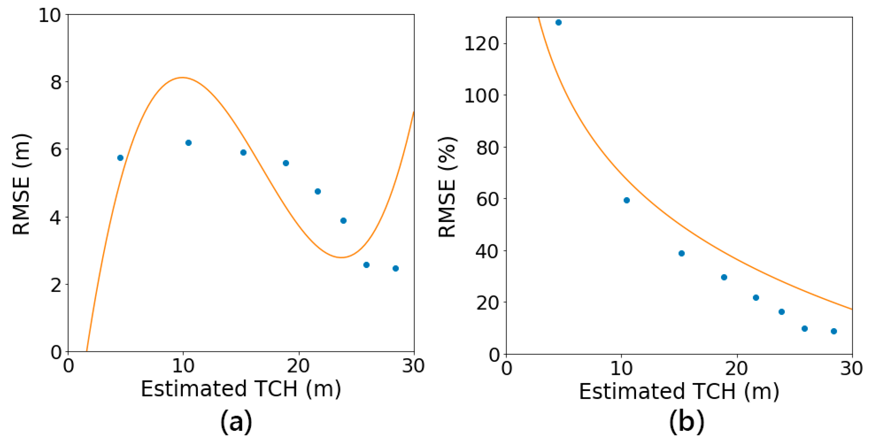
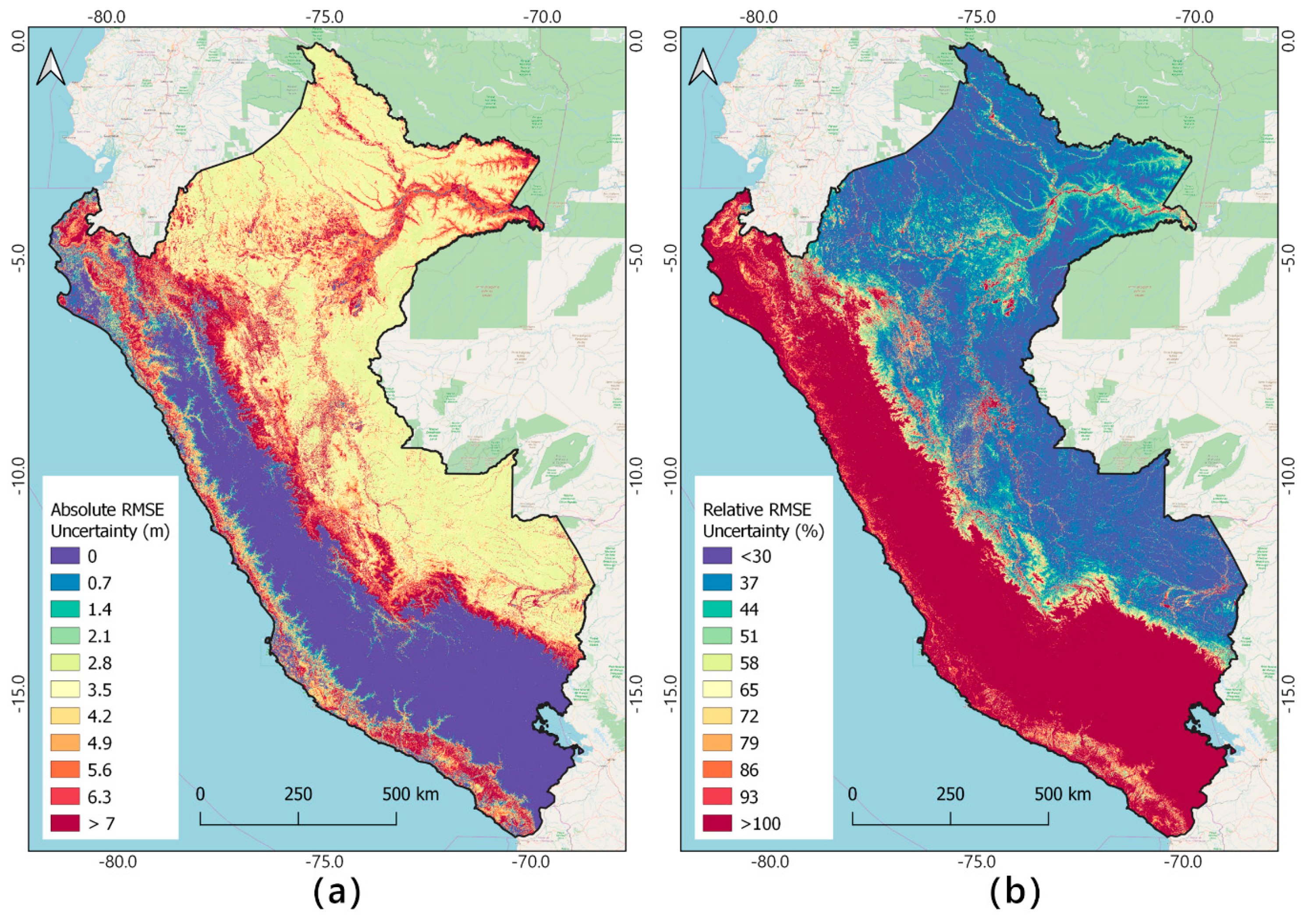
3.2. The Uncertainty of TCH Estimation

In addition to the R² and RMSE values of the TCH estimation, we generated spatially-explicit estimates of absolute RMSE (m) and relative RMSE uncertainty (%) of the estimated TCH (Figure 8, Figure 9). This was done by grouping the TCH into 10 bins by natural breaks and computing the RMSE values for each bin. To create wall-to-wall uncertainty maps for the entire area of Peru, we fitted a polynomial function (R² = 0.94, p-value = 0.001) and a logarithmic function (R² = 0.62, p-value = 0.011) for the absolute estimated uncertainty (Figure 8a) and the relative estimated uncertainty (Figure 8b), respectively. The absolute RMSE (m) declines from around 5–6 m for estimated TCH of 0–20 m towards 2.5 m for TCH values of 20–25 m. The error then abruptly increases for the highest TCH values due to the saturation in model predictions (Figure 8a). In terms of relative RMSE uncertainty, more than 50% error of the estimated TCH is characteristic for TCH values lower than 10 m. The error then lowers towards 10%–20% for estimated TCH values of 20–25 m (Figure 8b).

The spatial distribution of the absolute uncertainty shows that the higher errors (in m) correspond to the transition zones between lowland forest and Andean slopes, as well as to the wetlands and converted land use change areas (Figure 9a). Extremely sparse mountainous vegetation areas have high relative errors (>100%); however, the absolute errors for these areas are very low (<1 m). The areas with high TCH values have lower than 20% relative uncertainty, an important asset when the TCH estimations are further used to derive, for example, aboveground carbon density (Figure 9b). Overall, higher the estimated TCH, the lower the relative uncertainty, leading to high relative uncertainty for mountainous areas and low relative uncertainty for tropical forests.

4. Discussion

Our proposed high-resolution Peru-wide estimate of TCH resulted in an R² of 0.65 and RMSE of 4.36 m, comparable to other approaches available at different extents and resolutions. For example, Lefsky [49] used 500 m MODIS data with Geoscience Laser Altimeter System (GLAS) height transects to create a global forest canopy height map with an RMSE of 5.9 m. Using MODIS and GLAS data, Wang et al. [50] used a balanced RF algorithm at 500 m resolution to estimate a global mean forest canopy height with RMSEs of 2.7–4.4 m. Simard et al. [51] estimated global forest vertical structure at 1 km resolution using GLAS and ancillary data with RMSE of 6.1 m. Hansen et al. [52] used Landsat 7 and 8 with GLAS data to map the tree height in Sub-Saharan Africa with an overall mean absolute error (MAE) of 2.45 m. Qi et al. [53] estimated forest height by fusing TanDEM-X InSAR, simulated Global Ecosystem Dynamics Investigation (GEDI) canopy height, and digital terrain models to obtain an estimation with RMSEs of 4.0−6.7 m. In the context of the recently launched GEDI spaceborne LiDAR [10], the high spatial and temporal resolution of our approach will have significant contribution towards near-real-time monitoring of forest canopy height.

4.1. Model Performance

Parameter selection for model training is crucial for managing the model’s prediction performance when working with data prone to artifacts [54]. The addition of extra embedding dimensions, extra clusters, or the modification of landmark and projection chunk parameters can have negative effects on model behavior, despite achieving improved apparent performance. For example, despite utilizing the techniques above, an alternate set of parameters allows the model to differentiate mosaic components and reflect that in predictions. These artifacts persist at the country scale but are less severe.

Models trained over smaller regions (tested up to 100 × 100 km), based on the Fourier features mentioned above, were able to produce strong apparent R² and RMSE values, but behaved poorly when transferring the model to other regions. These results were misleading for a variety of factors, including high dimensionality of input features, comparatively low complexity of the output TCH prediction, spatially localized imaging artifacts in source data, and ecologically relevant spatial autocorrelations.

Underlying data and environmental challenges that were identified and addressed during this work suggest that interpreting results and uncertainties in prior modeling efforts requires careful consideration. In addition, despite the relative generalization success of the presented method, it is still an open question as to what degree are structure parameters discernable from Planet Dove textures.

4.2. Generalization Challenges

Research towards regional application of FOTO features to estimate aboveground biomass in central African forests have identified two main challenges: (i) variation in sensor and lighting parameters, and (ii) forest structural diversity [21]. When working specifically with Planet Dove normalized mosaics taken over Peru, generalizing a TCH estimation model for tropical rainforests involves addressing imaging challenges such as: (i) lighting inconsistencies across mosaic elements (sensor variation, atmospheric variation, preprocessing variation), and (ii) resolution inconsistencies across mosaic elements (angle from nadir, different sensors).

To operate at a large geographic scale, a model needs to be able to handle some of the challenges of using data collected across a highly varied ecosystem. These include: (i) the presence of forested and non-forested areas of an unspecified, and perhaps unknown variety of classes that are not labeled in advance; (ii) the presence of mixtures of those classes within 100 m cells, which produce continuous changes in output TCH simply due to coverage fraction; and (iii) highly unbalanced training data with respect to those classes and mixtures.

Further, the presence of ecologically-derived spatial correlations can compromise our ability to intuit generalization performance using a sampled validation set, when working on a smaller region. In a related effect, the high degree of similarity between plots can lead to minimal variances between sample distributions of both input attributes and prediction parameters, as well as correlation between input attributes used for prediction. As a result, the mechanisms employed by ensemble methods designed as variance reduction strategies, such as bagging or column subsampling (as part of RFs), may be compromised, leading to misleading estimates of generalization behavior.

4.2.1. Imaging Artifacts

The presence of the two categories of imaging artifacts represents a problematic combination for our texture features. Avoiding learning from inconsistent lighting involves ignoring the large length scale properties of the image, which are captured by the low frequency region of the power spectra. At the same time, avoiding learning from resolution inconsistencies in the Planet Dove mosaic involves ignoring small length scale behavior, which is captured by the high frequency region. In addition, when working with a mosaic, imaging artifacts present in constituent pieces can lead them to be identifiable, which can provide complex model location information, and defeat the model’s ability to generalize.

4.2.2. Environmental Challenges

The presence of challenges such as unspecified terrain types, climatic conditions, and regulatory limitations means that properly balanced and stratified sampling is nearly impossible to achieve. As a result, the application of machine learning algorithms without a mechanism for accounting for terrain types and mixtures via a land-use/land-cover (LULC) classification risks being biased towards the behavior of the oversampled class, even with ideally selected features. Decision tree-based machine learning techniques, in particular, are known to be sensitive to imbalanced training data [54]. While at smaller scales it may be possible to manually mask out forested areas for analysis, such efforts are impractical at a large geographic scale. Further, the presence of mixtures of terrain within grid cells of appropriate size for allometry may present a sizable question, because they do not properly represent a categorical variable and the allometric equations are not designed with mixtures in mind. In the future, a mixture modeling approach may be investigated to address this issue.

4.3. Limitations

Our proposed method is globally applicable and may be used to make predictions on new Planet Dove collections, enabling continuous monitoring of a region with imagery that has been prepared in the same way. To make predictions on new collections, images must be histogram-matched to the reference training mosaic. This is not ideal for many reasons. First, primary areas of interest are areas of change, where histogram matching is not very valid. Second, predictions are geographically constrained to the coverage of the training mosaic. Nevertheless, this technique has been implemented into the software package.

The time delay between the acquisition of LiDAR data (2011–2013) and the Planet Dove images (2018) may have influenced our results due to changes in land cover that occurred in this timeframe. The influence of this mismatch is minimized by the vast amount of data and by using an ensemble classifier that produces a number of decision trees by randomly selecting subsets of training samples and variables and is less sensitive to outliers. This influence is also minimized by using a resolution of 1 ha for our analysis.

5. Conclusions

We presented the technical and scientific challenges involved in the generation of reliable mechanisms for estimating TCH from Planet Dove satellite image spectral and textural features. We focused our methods on spatial texture analysis with modified FOTO textures and created a machine learning regression model using gradient boosted regression trees. Our developed software toolchain is a robust and generalizable regression model that provides an RMSE of 4.36 m in Peru. This represents a helpful advancement towards better monitoring of tropical forests, which can be further used for informing environmental policies and conservation actions.

References

1. Taubert, F.; Fischer, R.; Groeneveld, J.; Lehmann, S.; Müller, M.S.; Rödig, E.; Wiegand, T.; Huth, A. Global patterns of tropical forest fragmentation. Nature 2018, 554, 519–522. [Google Scholar] [CrossRef] [PubMed]
2. Mitchard, E.T.A. The tropical forest carbon cycle and climate change. Nature 2018, 559, 527–534. [Google Scholar] [CrossRef] [PubMed]
3. Asner, G.P.; Mascaro, J.; Anderson, C.; Knapp, D.E.; Martin, R.E.; Kennedy-Bowdoin, T.; van Breugel, M.; Davies, S.; Hall, J.S.; Muller-Landau, H.C.; et al. High-fidelity national carbon mapping for resource management and REDD+. Carbon Balance Manag. 2013, 8, 7. [Google Scholar] [CrossRef] [PubMed] [Green Version]
4. Bos, A.B.; De Sy, V.; Duchelle, A.E.; Herold, M.; Martius, C.; Tsendbazar, N.-E. Global data and tools for local forest cover loss and REDD+ performance assessment: Accuracy, uncertainty, complementarity and impact. Int. J. Appl. Earth Obs. Geoinf. 2019, 80, 295–311. [Google Scholar] [CrossRef]
5. Brodrick, P.G.; Davies, A.B.; Asner, G.P. Uncovering Ecological Patterns with Convolutional Neural Networks. Trends Ecol. Evol. 2019, 34, 734–745. [Google Scholar] [CrossRef]
6. Chave, J.; Andalo, C.; Brown, S.; Cairns, M.A.; Chambers, J.Q.; Eamus, D.; Fölster, H.; Fromard, F.; Higuchi, N.; Kira, T.; et al. Tree allometry and improved estimation of carbon stocks and balance in tropical forests. Oecologia 2005, 145, 87–99. [Google Scholar] [CrossRef]
7. Newnham, G.J.; Armston, J.D.; Calders, K.; Disney, M.I.; Lovell, J.L.; Schaaf, C.B.; Strahler, A.H.; Danson, F.M. Terrestrial laser scanning for plot-scale forest measurement. Curr. For. Rep. 2015, 1, 239–251. [Google Scholar] [CrossRef] [Green Version]
8. Asner, G.P.; Knapp, D.E.; Boardman, J.; Green, R.O.; Kennedy-Bowdoin, T.; Eastwood, M.; Martin, R.E.; Anderson, C.; Field, C.B. Carnegie airborne observatory-2: Increasing science data dimensionality via high-fidelity multi-sensor fusion. Remote Sens. Environ. 2012, 124, 454–465. [Google Scholar] [CrossRef]
9. Tang, H.; Armston, J.; Hancock, S.; Marselis, S.; Goetz, S.; Dubayah, R. Characterizing global forest canopy cover distribution using spaceborne lidar. Remote Sens. Environ. 2019, 231, 111262. [Google Scholar] [CrossRef]
10. Dubayah, R.; Blair, J.B.; Goetz, S.; Fatoyinbo, L.; Hansen, M.; Healey, S.; Hofton, M.; Hurtt, G.; Kellner, J.; Luthcke, S.; et al. The Global Ecosystem Dynamics Investigation: High-resolution laser ranging of the Earth’s forests and topography. Sci. Remote Sens. 2020, 1, 100002. [Google Scholar] [CrossRef]
11. Wang, Z.; Schaaf, C.B.; Lewis, P.; Knyazikhin, Y.; Schull, M.A.; Strahler, A.H.; Yao, T.; Myneni, R.B.; Chopping, M.J.; Blair, B.J. Retrieval of canopy height using moderate-resolution imaging spectroradiometer (MODIS) data. Remote Sens. Environ. 2011, 115, 1595–1601. [Google Scholar] [CrossRef] [Green Version]
12. Sawada, Y.; Suwa, R.; Jindo, K.; Endo, T.; Oki, K.; Sawada, H.; Arai, E.; Shimabukuro, Y.E.; Celes, C.H.S.; Campos, M.A.A.; et al. A new 500-m resolution map of canopy height for Amazon forest using spaceborne LiDAR and cloud-free MODIS imagery. Int. J. Appl. Earth Obs. Geoinf. 2015, 43, 92–101. [Google Scholar] [CrossRef] [Green Version]
13. Staben, G.; Lucieer, A.; Scarth, P. Modelling LiDAR derived tree canopy height from Landsat TM, ETM+ and OLI satellite imagery—A machine learning approach. Int. J. Appl. Earth Obs. Geoinf. 2018, 73, 666–681. [Google Scholar] [CrossRef]
14. Hudak, A.T.; Lefsky, M.A.; Cohen, W.B.; Berterretche, M. Integration of lidar and Landsat ETM+ data for estimating and mapping forest canopy height. Remote Sens. Environ. 2002, 82, 397–416. [Google Scholar] [CrossRef] [Green Version]
15. Avitabile, V.; Baccini, A.; Friedl, M.A.; Schmullius, C. Capabilities and limitations of Landsat and land cover data for aboveground woody biomass estimation of Uganda. Remote Sens. Environ. 2012, 117, 366–380. [Google Scholar] [CrossRef]
16. Reiche, J.; Hamunyela, E.; Verbesselt, J.; Hoekman, D.; Herold, M. Improving near-real time deforestation monitoring in tropical dry forests by combining dense Sentinel-1 time series with Landsat and ALOS-2 PALSAR-2. Remote Sens. Environ. 2018, 204, 147–161. [Google Scholar] [CrossRef]
17. Planet Team. Planet Application Program Interface: In Space for Life on Earth; Planet Team: San Francisco, CA, USA, 2017. [Google Scholar]
18. Wood, E.M.; Pidgeon, A.M.; Radeloff, V.C.; Keuler, N.S. Image texture as a remotely sensed measure of vegetation structure. Remote Sens. Environ. 2012, 121, 516–526. [Google Scholar] [CrossRef]
19. Solórzano, J.V.; Gallardo-Cruz, J.A.; González, E.J.; Peralta-Carreta, C.; Hernández-Gómez, M.; de Oca, A.F.-M.; Cervantes-Jiménez, L.G. Contrasting the potential of Fourier transformed ordination and gray level co-occurrence matrix textures to model a tropical swamp forest’s structural and diversity attributes. J. Appl. Remote Sens. 2018, 12, 036006. [Google Scholar] [CrossRef]
20. Haralick, R.M.; Shanmugam, K.; Dinstein, I. Textural features for image classification. IEEE Trans. Syst. Man Cybern. 1973, SMC-3, 610–621. [Google Scholar] [CrossRef] [Green Version]
21. Bastin, J.F.; Barbier, N.; Couteron, P.; Adams, B.; Shapiro, A.; Bogaert, J.; De Cannière, C. Aboveground biomass mapping of African forest mosaics using canopy texture analysis: Toward a regional approach. Ecol. Appl. 2014, 24, 1984–2001. [Google Scholar] [CrossRef]
22. Couteron, P.; Pelissier, R.; Nicolini, E.A.; Paget, D. Predicting tropical forest stand structure parameters from Fourier transform of very high-resolution remotely sensed canopy images. J. Appl. Ecol. 2005, 42, 1121–1128. [Google Scholar] [CrossRef] [Green Version]
23. Singh, M.; Evans, D.; Friess, D.A.; Tan, B.S.; Nin, C.S. Mapping above-ground biomass in a tropical forest in Cambodia using canopy textures derived from Google Earth. Remote Sens. 2015, 7, 5057–5076. [Google Scholar] [CrossRef] [Green Version]
24. Asner, G.P.; Mascaro, J. Mapping tropical forest carbon: Calibrating plot estimates to a simple LiDAR metric. Remote Sens. Environ. 2014, 140, 614–624. [Google Scholar] [CrossRef]
25. Asner, G.P.; Knapp, D.E.; Martin, R.E.; Tupayachi, R.; Anderson, C.B.; Mascaro, J.; Sinca, F.; Chadwick, K.D.; Higgins, M.; Farfan, W.; et al. Targeted carbon conservation at national scales with high-resolution monitoring. Proc. Natl. Acad. Sci. USA 2014, 111, E5016–E5022. [Google Scholar] [CrossRef] [Green Version]
26. Csillik, O.; Kumar, P.; Mascaro, J.; O’Shea, T.; Asner, G.P. Monitoring tropical forest carbon stocks and emissions using Planet satellite data. Sci. Rep. 2019, 9, 17831. [Google Scholar] [CrossRef] [Green Version]
27. Csillik, O.; Asner, G.P. Aboveground carbon emissions from gold mining in the Peruvian Amazon. Environ. Res. Lett. 2020, 15, 014006. [Google Scholar] [CrossRef]
28. Ter Steege, H.; Pitman, N.C.A.; Phillips, O.L.; Chave, J.; Sabatier, D.; Duque, A.; Molino, J.-F.; Prévost, M.-F.; Spichiger, R.; Castellanos, H.; et al. Continental-scale patterns of canopy tree composition and function across Amazonia. Nature 2006, 443, 444–447. [Google Scholar] [CrossRef]
29. Gentry, A.H. Tree species richness of upper Amazonian forests. Proc. Natl. Acad. Sci. USA 1988, 85, 156–159. [Google Scholar] [CrossRef] [Green Version]
30. Jarvis, A.; Guevara, E.; Reuter, H.I.; Nelson, A.D. Hole-Filled SRTM for the Globe: Version 4: Data Grid; CGIAR Consortium for Spatial Information: Montpellier, France, 2008. [Google Scholar]
31. Planet Team. Planet Imagery Product Specifications; Planet Team: San Francisco, CA, USA, 2018. [Google Scholar]
32. Barbier, N.; Couteron, P.; Proisy, C.; Malhi, Y.; Gastellu-Etchegorry, J.-P. The variation of apparent crown size and canopy heterogeneity across lowland Amazonian forests: Amazon forest canopy properties. Glob. Ecol. Biogeogr. 2010, 19, 72–84. [Google Scholar] [CrossRef]
33. Ploton, P.; Pélissier, R.; Proisy, C.; Flavenot, T.; Barbier, N.; Rai, S.N.; Couteron, P. Assessing aboveground tropical forest biomass using Google Earth canopy images. Ecol. Appl. 2012, 22, 993–1003. [Google Scholar] [CrossRef] [Green Version]
34. Fowlkes, C.; Belongie, S.; Chung, F.; Malik, J. Spectral grouping using the Nyström method. IEEE Trans. Pattern Anal. Mach. Intell. 2004, 26, 214–225. [Google Scholar] [CrossRef] [Green Version]
35. Kruse, F.A.; Lefkoff, A.B.; Boardman, J.W.; Heidebrecht, K.B.; Shapiro, A.T.; Barloon, P.J.; Goetz, A.F.H. The spectral image processing system (SIPS)—Interactive visualization and analysis of imaging spectrometer data. Remote Sens. Environ. 1993, 44, 145–163. [Google Scholar] [CrossRef]
36. Breiman, L. Random forests. Mach. Learn. 2001, 45, 5–32. [Google Scholar] [CrossRef] [Green Version]
37. Gislason, P.O.; Benediktsson, J.A.; Sveinsson, J.R. Random forests for land cover classification. Pattern Recognit. Lett. 2006, 27, 294–300. [Google Scholar] [CrossRef]
38. Juel, A.; Groom, G.B.; Svenning, J.-C.; Ejrnæs, R. Spatial application of Random Forest models for fine-scale coastal vegetation classification using object based analysis of aerial orthophoto and DEM data. Int. J. Appl. Earth Obs. Geoinf. 2015, 42, 106–114. [Google Scholar] [CrossRef]
39. Jin, S.; Su, Y.; Gao, S.; Hu, T.; Liu, J.; Guo, Q. The transferability of Random Forest in canopy height estimation from multi-source remote sensing data. Remote Sens. 2018, 10, 1183. [Google Scholar] [CrossRef] [Green Version]
40. Lennon, J.J. Red-shifts and red herrings in geographical ecology. Ecography 2000, 23, 101–113. [Google Scholar] [CrossRef]
41. Hawkins, B.A.; Diniz-Filho, J.A.F.; Mauricio Bini, L.; De Marco, P.; Blackburn, T.M. Red herrings revisited: Spatial autocorrelation and parameter estimation in geographical ecology. Ecography 2007, 30, 375–384. [Google Scholar] [CrossRef]
42. Diniz-Filho, J.A.F.; Bini, L.M.; Hawkins, B.A. Spatial autocorrelation and red herrings in geographical ecology: Spatial autocorrelation in geographical ecology. Glob. Ecol. Biogeogr. 2003, 12, 53–64. [Google Scholar] [CrossRef] [Green Version]
43. Tang, C.; Garreau, D.; von Luxburg, U. When do random forests fail. In Advances in Neural Information Processing Systems 31; Bengio, S., Wallach, H., Larochelle, H., Grauman, K., Cesa-Bianchi, N., Garnett, R., Eds.; Curran Associates, Inc.: New York, NY, USA, 2018; pp. 2983–2993. [Google Scholar]
44. Ashcroft, N.W.; Mermin, N.D. Solid State Physics: Cengage Learning; Cengage Learning: Boston, MA, USA, 2011; ISBN 9788131500521. [Google Scholar]
45. Ho, T.K. The random subspace method for constructing decision forests. IEEE Trans. Pattern Anal. Mach. Intell. 1998, 20, 832–844. [Google Scholar]
46. Friedman, J.H. Greedy function approximation: A gradient boosting machine. Ann. Stat. 2001, 29, 1189–1232. [Google Scholar] [CrossRef]
47. Ng, A.Y.; Jordan, M.I.; Weiss, Y. On Spectral Clustering: Analysis and an algorithm. In Advances in Neural Information Processing Systems 14; Dietterich, T.G., Becker, S., Ghahramani, Z., Eds.; MIT Press: Cambridge, MA, USA, 2002; pp. 849–856. [Google Scholar]
48. Puzicha, J.; Hofmann, T.; Buhmann, J.M. Non-parametric similarity measures for unsupervised texture segmentation and image retrieval. In Proceedings of the IEEE Computer Society Conference on Computer Vision and Pattern Recognition, San Juan, PR, USA, 17–19 June 1997; pp. 267–272. [Google Scholar]
49. Lefsky, M.A. A global forest canopy height map from the moderate resolution imaging spectroradiometer and the geoscience laser altimeter system. Geophys. Res. Lett. 2010, 37. [Google Scholar] [CrossRef] [Green Version]
50. Wang, Y.; Li, G.; Ding, J.; Guo, Z.; Tang, S.; Wang, C.; Huang, Q.; Liu, R.; Chen, J.M. A combined GLAS and MODIS estimation of the global distribution of mean forest canopy height. Remote Sens. Environ. 2016, 174, 24–43. [Google Scholar] [CrossRef]
51. Simard, M.; Pinto, N.; Fisher, J.B.; Baccini, A. Mapping forest canopy height globally with spaceborne lidar. J. Geophys. Res. 2011, 116, 248. [Google Scholar] [CrossRef]
52. Hansen, M.C.; Potapov, P.V.; Goetz, S.J.; Turubanova, S.; Tyukavina, A.; Krylov, A.; Kommareddy, A.; Egorov, A. Mapping tree height distributions in Sub-Saharan Africa using Landsat 7 and 8 data. Remote Sens. Environ. 2016, 185, 221–232. [Google Scholar] [CrossRef] [Green Version]
53. Qi, W.; Lee, S.-K.; Hancock, S.; Luthcke, S.; Tang, H.; Armston, J.; Dubayah, R. Improved forest height estimation by fusion of simulated GEDI Lidar data and TanDEM-X InSAR data. Remote Sens. Environ. 2019, 221, 621–634. [Google Scholar] [CrossRef] [Green Version]
54. Belgiu, M.; Dragut, L. Random forest in remote sensing: A review of applications and future directions. ISPRS J. Photogramm. Remote Sens. 2016, 114, 24–31. [Google Scholar] [CrossRef]
Figure 1. (a) The source data used were a 4-band Planet Dove normalized mosaic, shown in false color, together with (b) Shuttle Radar Topography Mission (SRTM) elevation data. Features derived from these two data sets are used to estimate (b) top-of-canopy height (TCH) as measured by the Global Airborne Observatory (GAO) light detection and ranging (LiDAR) surveys, shown in black paths.
Remotesensing 12 01160 g001
Figure 2. The workflow for TCH estimation using Planet Dove, elevation, and airborne LiDAR datasets. The Planet Dove high-resolution mosaic was used as input for the Fourier textural ordination (FOTO) and spectral projection in order to generate features for the gradient boosted regression model weighted based on K-means clusters. The final TCH estimation was validated against hold-out airborne LiDAR measurements of TCH.
Remotesensing 12 01160 g002
Figure 3. (a) The Planet Dove red, green, blue (RGB) and (b) its green channel of a 1 ha image subset, (c) the latter decomposed into its Fourier components at different wavelengths (WLs). Real-space visualizations of the component textures of the patch are displayed. The radial power spectra components, which are used as features, measure the amount of signal in the image patch allocated to each component length scale.
Remotesensing 12 01160 g003
Figure 4. Sampled image patches from K-means clustering of the spectral projection. This clustering generated an unsupervised rough terrain classification that appears to group forested, mixture, and various unforested states into categories with a range of different average TCH values. These clusters were used as a proxy for the implicit categorical variable that partially drives the continuous TCH variable and were used to inform an inverse-frequency weighting scheme used during model fitting.
Remotesensing 12 01160 g004
Figure 5. The model produces a country-wide estimation of TCH with R2 = 0.65 and root mean square error (RMSE) of 4.36 m on 20% LiDAR-based TCH validation samples. Training parameters were 20 Fourier bins, 8 clusters, 6 dimensions, 3000 landmarks, and 600 projection samples. These parameters were chosen to balance learning image artifacts and minimize the RMSE. Note that the estimated TCH values are of the integer type.
Remotesensing 12 01160 g005
Figure 6. The TCH estimation map of Peru at 1 ha spatial resolution (100 × 100 m pixels) with subsets (a–i) shown in Figure 7. A comparison between our TCH estimation and transects of airborne LiDAR TCH is shown on the right side of the figure.
Remotesensing 12 01160 g006
Figure 7. Subsets with different TCH distribution, with locations shown in Figure 6: (a) Intact forest in Loreto; (b) transition between flooded and terra firme forest in Loreto; (c) swamp forest in Loreto; (d) Andean tree line in Cusco; (e) logging roads and deforestation in Ucayali; (f) deforestation near Puerto Maldonado in Madre de Dios; (g) gold mining in Madre de Dios; (h) oil palm plantations and agriculture near Pucallpa in Ucayali; and (i) intense deforestation south of Pucallpa in Ucayali.
Remotesensing 12 01160 g007
Figure 8. (a) Absolute RMSE uncertainty (in m) and (b) the relative RMSE uncertainty (% of estimated TCH).
Remotesensing 12 01160 g008
Figure 9. (a) Absolute estimated RMSE uncertainty (in m) and (b) relative estimated RMSE uncertainty (in % of estimated TCH) for all of Peru.
Remotesensing 12 01160 g009