1. Introduction
Mapping technologies that allow vineyard managers to better understand variability in the vineyard have proliferated in recent years. A commonly used method for mapping vineyards is normalized difference vegetation index (NDVI) [
1] which can be acquired through satellite imagery, overhead flight by plane or drone, or ground based sensing. NDVI variability maps have enabled more directed cultural practices such as selective harvest, but also offer an improvement in the efficacy of experimental protocols [
2,
3].
Spatial patterns in agricultural plots were acknowledged well before they could be imaged [
4,
5], resulting in the use of randomized complete block designs (RCBD) to compensate. More recently, researchers have realized that RCBD designs are susceptible to bias resulting from periodicity and spatial autocorrelation [
6], resulting in recommendations for use of spatially-balanced (i.e., non-random) designs [
7].
A wide range of parameters tend to be sampled in vineyards, such as soil, vine growth, and fruit composition. Vine sampling protocols have been modified by researchers to compensate for unknown spatial variability within the canopy [
8,
9,
10] and more recently to directly sample a known measured population distribution in winegrape canopies by designing sampling protocols that seek to optimize the balance between sample size and fit to population [
11].
The sampling protocol described by [
11] leveraged a manually collected dataset of approximately 800 fruit cluster sunlight exposure values, as determined by enhanced point quadrat analysis [
12], to demonstrate that whole-block sample sizes could be reduced by up 60% compared to random sampling. Optimization of sampling operations using known spatial patterns can lead to a lower information cost [
13].
Substituting a stratified sampling method, designed to reduce the labor effort by reducing the number of vines sampled, has been shown to produce samples of similar quality to the typical industry standard of random sampling when measuring the commonly monitored fruit quality parameters of Brix (a measure of soluble solids as proxy for sugar), pH, total acidity, and color [
14]. Further reduction in sampling locations to a single vineyard row within a block can both reduce the labor required to collect the sample [
2]. The sampling protocols described in [
2] demonstrated the use of 0.5-m pixel-scale aerial NDVI imagery to compute an optimal sampling strategy by directing sampling to a set of spatially explicit pixel locations. These protocols, which were designed to maximize sample fitness (i.e., ensuring that sampling was maximally reflective of known population distributions) have heretofore not been rigorously compared with other sampling methods in a field trial.
Furthermore, despite the theoretical efficiency gains, requiring a field technician to sample with such a high degree of spatial precision has practical limitations both in the time required to find the prescribed locations, and in ability to consistently sample with the specified spatial precision. It is desirable to develop sampling methods that are both spatially rigorous but also resilient to the behavioral inconsistencies of human field technicians.
This study seeks to improve upon existing best practices for sampling by using satellite NDVI vineyard imagery to compute optimal spatially-explicit sampling protocols that minimize the number of locations sampled while maximizing fitness of sample to population. In particular, the objectives of this work were to conduct field experiments to determine (1) if the algorithms from our previous work [
11] would scale to larger data sets such as whole-block NDVI and; (2) if sampling efficiency could be improved, compared to both previous stratified protocols and random sampling, by further reducing the total number of sampling locations and the distance between them.
2. Materials and Methods
2.1. Satellite NDVI Imagery
All NDVI imagery was LANDSAT 7 30-m scale images (each pixel covers 900 square meters of land) captured near early veraison (onset of fruit ripening) between 2012 and 2016 and selected for minimal cloud cover. Experimental vineyard blocks were bounded by shapefiles created using ArcMap (Version 10.5, Esri, Redlands, CA) which were manually processed to eliminate features such as access roads, buildings, and intra-block trees from the block image pixels. NDVI values were calculated using the red (R) and near infrared (NIR) bands of the Landsat data using the formula (NIR-R)/(NIR+R) and normalized to a range of zero to one to simplify computation. Images were not processed for atmospheric correction or otherwise calibrated across vineyards, as variability was only measured and analyzed locally within each vineyard block. Study areas were not affected by the scan line corrector failure.
2.2. Vineyards
All experimental vineyards were in California’s Central Valley. In 2016, 13 blocks were selected for use in studying the proposed sampling protocol (
Table 1). In 2017, 24 blocks were selected. Of the 24 blocks selected for 2017, 16 were used for studying the efficacy of the proposed sampling protocol compared to random sampling. All 24 were used to conduct a temporal stability analysis for the four seasons 2013 and 2016 inclusive.
2.3. Sampling Protocols
Three sampling protocols (
Table 2) were employed in the study: (1) a random sample collected from 20 locations (R20); (2) a pre-existing stratified sampling protocol known as "commercial maturity" that sampled from four locations of two NDVI pixels each for a total of eight pixels (CM8); and (3) a proposed spatially-explicit method that samples from a single location, but includes three consecutive NDVI pixels (NDVI3). Both CM8 and NDVI3 were compared to R20 as a quality reference.
2.3.1. R20
Twenty locations were randomly chosen via custom software (MATLAB version 2017a, MathWorks, Natick, MA, USA). Locations were computed by selecting 20 random pixels from the block shapefile, then applying a random offset of −14 to +14 m to both the X and Y location. Vineyard edges were avoided by limiting the centroid offsets to the range of either −14 to 0 m or 0 to +14 m when the pixel was on an edge of the block. The field technician was guided to each sampling location via a GPS enabled smart phone or tablet. One fruit cluster was collected from each location, chosen by blindly reaching into the canopy at the location indicated by the GPS locating device, resulting in a total of 20 clusters per block. All clusters collected were combined to create one biological sample for each block. In 2016, all 13 blocks were sampled using the R20 protocol as close to harvest date as possible. In 2017, 16 of the 24 vineyard blocks were sampled using the R20 protocol at two different dates—one early in veraison and one close to harvest.
2.3.2. CM8
Four locations were chosen for each block, each representing a quadrant of the block, defined by the GPS location of vineyard row end-post. The field technician was guided to each sampling location via a GPS enabled smart phone or tablet. Vineyard edges were avoided by pacing off approximately 30 m (i.e., one NDVI pixel) before starting sample collection. Sampling started here, and the field technician walked at a measured pace for the length of two pixels, stopping to collect a fruit cluster every 10 steps, chosen by blindly reaching into the canopy, on alternate sides of the row. This resulted in a sample of 5 fruit clusters per each of the 4 locations (2 pixels each) for a total of 20 clusters per block. All clusters collected were combined to create one biological sample for each block. In 2016, all 13 experimental blocks were sampled using the CM8 protocol as close to harvest date as possible. In 2017, 16 experimental vineyard blocks were sampled using the CM8 protocol weekly between veraison and harvest.
2.3.3. NDVI3
Field technicians were directed to a specific location in the vineyard block where they walked at a measured pace, blindly selecting fruit clusters from alternate sides of the row middle over a distance of 90 m (three pixels)—collecting a total of 20 clusters across all three pixels. All clusters collected were combined to create one biological sample for each block. Locations were determined using Landsat NDVI image obtained from dates during the previous season phenological stage of veraison. As a result, a “current” solution for a block in 2017 is based on NDVI imagery from 2016. Sampling solutions were calculated based on previous seasons to allow for the determination of NDVI3 sampling protocols in a current season before the onset of veraison, allowing sampling to start earlier.
In 2016, the sampling location was determined by using custom software (MATLAB, MathWorks, Natick, MA, USA) to perform the following algorithm, the result of which is illustrated by
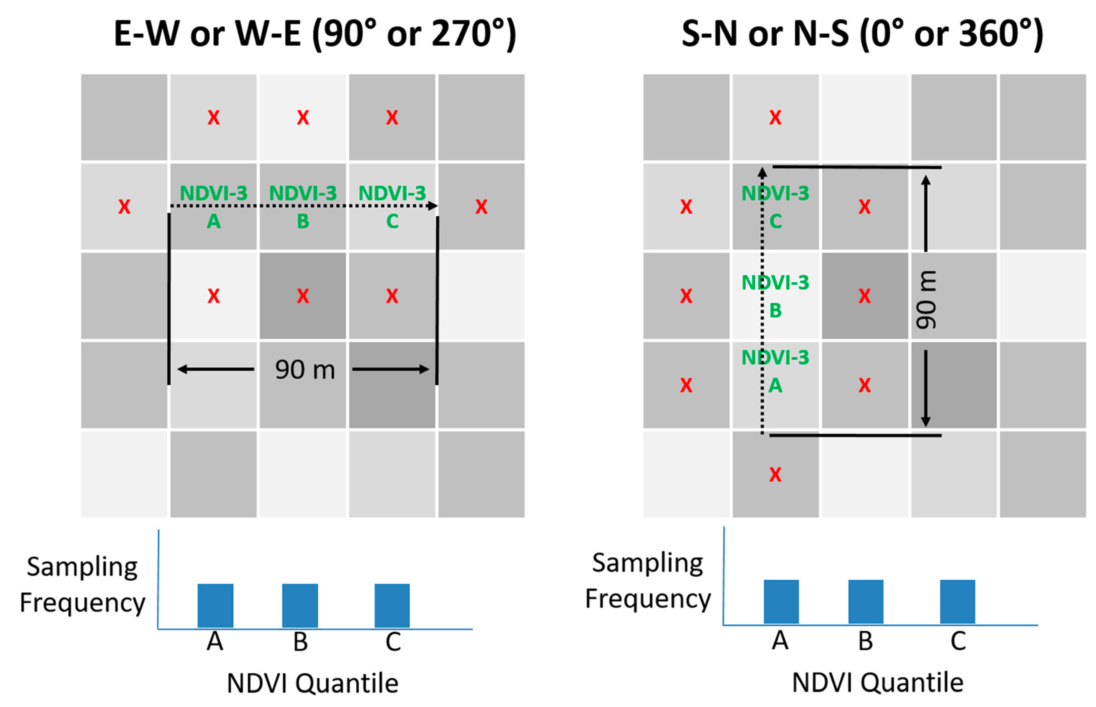
Figure 1, for vineyards planted in either east–west or north–south orientation: (1) three quantile means were computed for the NDVI block image representing the left tail, center, and right tail of the population by sorting the pixel values in ascending order, dividing all values into three equal-sized bins and averaging the values; (2) the block NDVI image was analyzed, three pixels at a time, to quantify how well those three pixels fit the target tercile means by calculating the sum of the three quantile errors. The quantile error for each pixel was computed as the percent difference compared to the target value. The center pixel was always compared to the center quantile. The first and third quantiles did not need to appear in order; (3) to account for the possibility that a field technician might over-sample or under-sample the beginning or end of the 90 m sampling region, the center pixel always represents the middle quantile, ensuring that the center quantile would not be under-sampled or over-sampled; (4) after all pixel combinations were analyzed, the combination with the lowest sum of errors was chosen as the best solution.
In 2017, vineyards were included that were planted at row angles other than North–South or East–West, for angled rows, 90 m of sampling length necessarily resulted in an unequal distribution among NDVI pixels leading to the following modified algorithm, as illustrated by
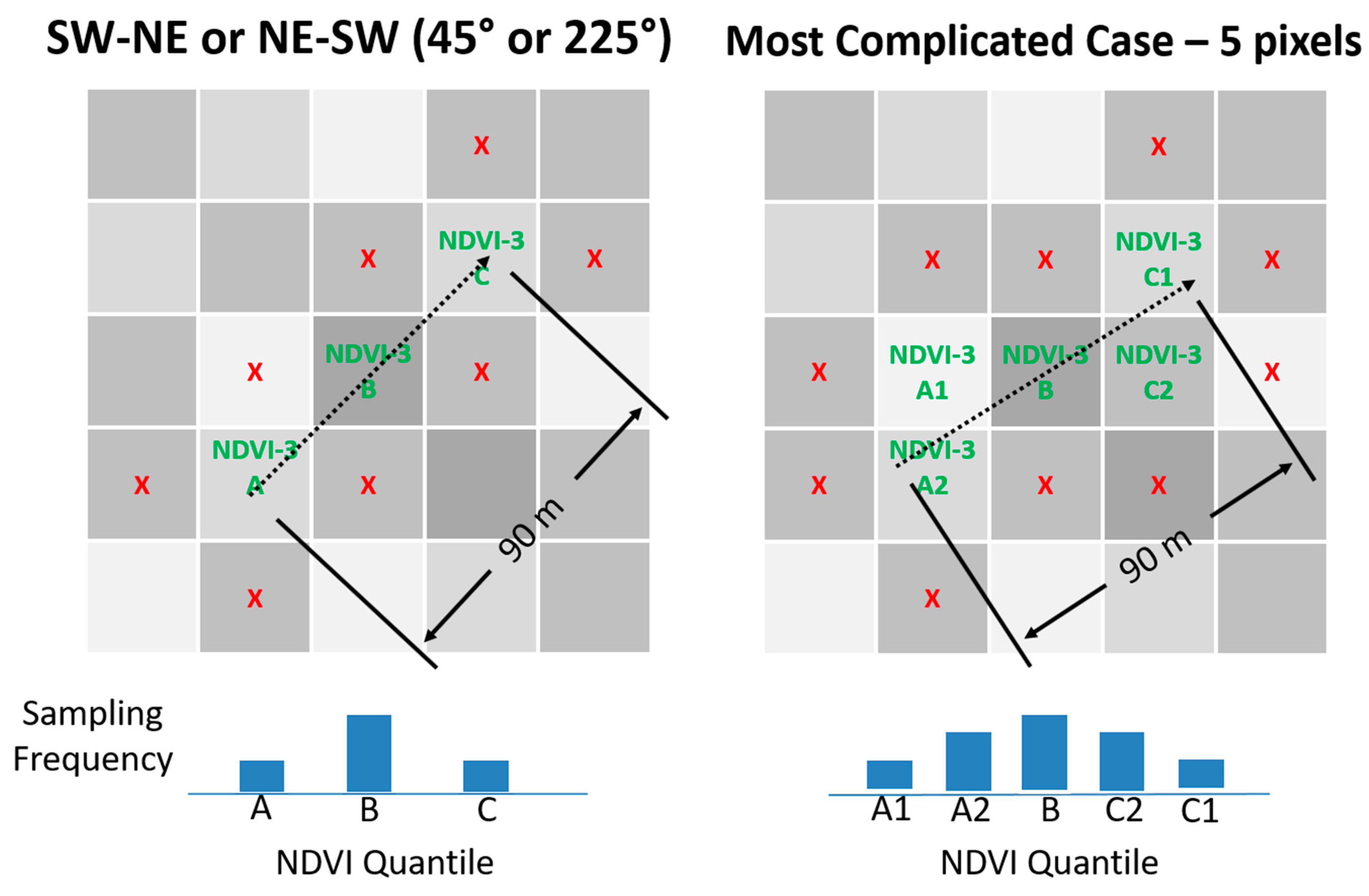
Figure 2: (1) three quantile means were computed for the NDVI block image representing the left tail, center, and right tail of the population by sorting the pixel values in ascending order, dividing all values into three equal-sized bins and averaging the values; (2) the block NDVI image was analyzed, nine pixels at time, to quantify how well those nine pixels fit the target quantile means by calculating the sum of the three quantile errors. The quantile error for each pixel was computed as the percent difference compared to the target value. The center pixel was always compared to the center quantile. The one or two pixels to either side of the center were compared to the tail quantiles using a weighted average which was weighted by length of travel within the pixel. The first and third quantiles did not need to appear in order; (3) row orientation was considered to ensure that the three adjacent pixels were those that would be naturally traversed by a field technician walking down the vineyard row; (4) to account for the possibility that the field technician might over-sample or under-sample the beginning or end of the 90 m sampling region, the center pixel was always tested against the middle quantile—ensuring that the center quantile was never under-sampled or over-sampled; (5) after all pixel combinations were analyzed, the combination with the lowest sum of errors was chosen as the best solution. The modified algorithm for 2017 superseded the 2016 algorithm as it covered the simpler cases with equivalent results.
2.4. Fruit Composition
In 2016, fruit samples were analyzed to quantify Brix and titratable acidity (TA). In 2017, fruit samples were analyzed to quantify Brix, TA, pH, and total anthocyanins. Chemical analysis was performed using proprietary protocols.
2.5. Comparison of Sampling Protocols
All statistics were performed using MATLAB (version 2017a, Natick, MA, USA). Pearson Correlation Coefficients (N = 13 vineyards in 2016, N = 16 vineyards in 2017) were used to compare fruit chemistry measurements between R20 and CM8, and between R20 and NDVI3. Two-value Kolmogorov-Smirnov testing was used to compare sampled pixels to block population pixels [
15]. An example of a vineyard image and processing is shown in
Figure 3.
2.6. Temporal Stability of NDVI3 Sampling Protocols
Temporal Stability of NDVI3 sampling solutions was tested by computing the best sampling location for the 24 experiments blocks (
Table 1) in 4 consecutive years using Landsat imagery. For each block, the best solution was computed for each of the four years, then each of those four sampling locations was applied to the Landsat imagery in all four years to determine how well a location computed for any given year performed in the other three years. For each block-year pairing, random sampling was simulated by randomly selecting 100 locations and the performance of NDVI3 solutions was compared to the random samples.
3. Results
3.1. Correlations Among Sampling Methods
Pearson Correlation Coefficients between R20 and CM8, and between R20 and NDVI3 are shown in
Table 3. In 2016 correlations were high, suggesting that both CM8 and NDVI3 were suitable alternatives to R20 for measuring Brix, TA, and total anthocyanins. In 2017, correlations were high at the first R20 sampling date with R20 vs NDVI3 underperforming CM8 for anthocyanin measurement. At the second R20 sampling NDVI3 consistently outperformed CM8 for all measured variables, with the Brix correlation being particularly low for CM8 (R = −0.05). This poor correlation, as well as the reduced correlation of NDVI3 at the second R20 sampling may be partially explained by the restricted range of Brix value across all blocks closer to harvest (R20 Brix ranged from 18.4 to 24.1 for a spread of 5.7 at the first sampling and from 22.9 to 25.4 for a spread of 2.5 at the second). Similarly, the marked improvement in anthocyanin correlations for NDVI3 in the second R20 sampling, compared to the first R20 sampling, may be partially explained by the widening of anthocyanin value ranges closer to harvest (R20 total anthocyanin ranged from 0.51 to 1.18 for a spread of 0.67 at the first sampling and from 0.62 to 1.53 for a spread of 0.91 at the second).
3.2. Sample Fitness
For 12 of the 13 blocks, the K-S test p value was lower for CM8 than for NDVI3, indicating a poorer fit (higher p values = better fit as the function was implemented in MATLAB) (
Table 4). In three blocks, p < 0.05 for CM8 which indicated a failure of the sample to represent the block population. R20 outperformed CM8 in 10 of the 13 blocks as indicated by the K-S test. Percentage of block pixels sampled ranged from 0.4 to 6.3 for NDVI3 with a mean of 1.9, from 1.1 to 16.7 with a mean of 5.0 for CM8, and from 2.7 to 41.7 for R20 with a mean of 12.6. No significant correlation was found between number of pixels within the block and K-S performance (R = 0.06, −0.21. and 0.07 for R20, CM8, and NDVI3, respectively), suggesting that block size was not a predictor of sample fitness. All NDVI3 solutions in 2017 passed the K-S test (data not shown).
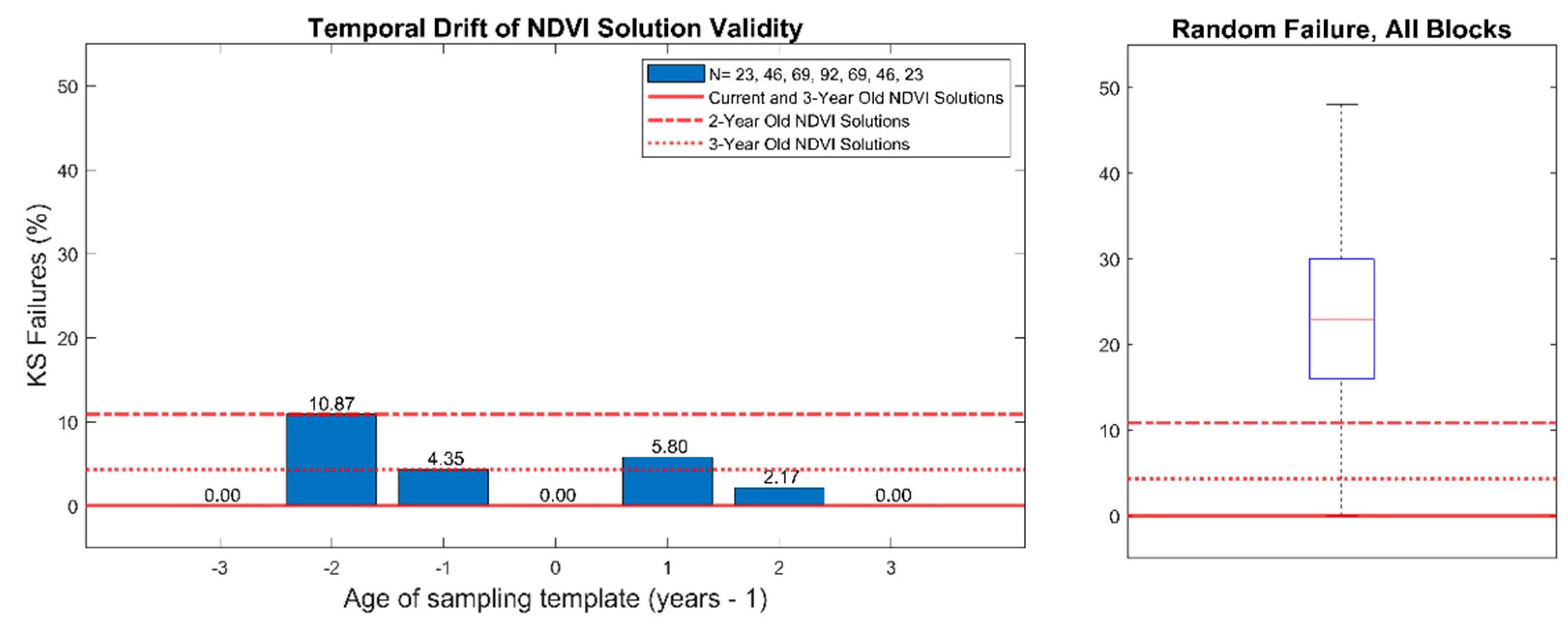
Temporal stability of NDVI3 solutions is shown in
Figure 4. Block 2017-06 was removed from the analysis because the small size and narrow block geometry constrained the universe of all possible NDVI3 solutions to a single solution. All 23 remaining blocks passed the K-S test when NDVI3 solutions were computed using NDVI imagery from the previous year. When NDVI3 solutions were calculated based on two-year old, three-year old, and four-year old imagery, there were K-S failure rates of 4%, 11%, and 0%, respectively. When current NDVI solutions were applied to imagery from two prior, three prior, and four prior years, K-S failure rates were 5%, 2%, and 0% respectively.
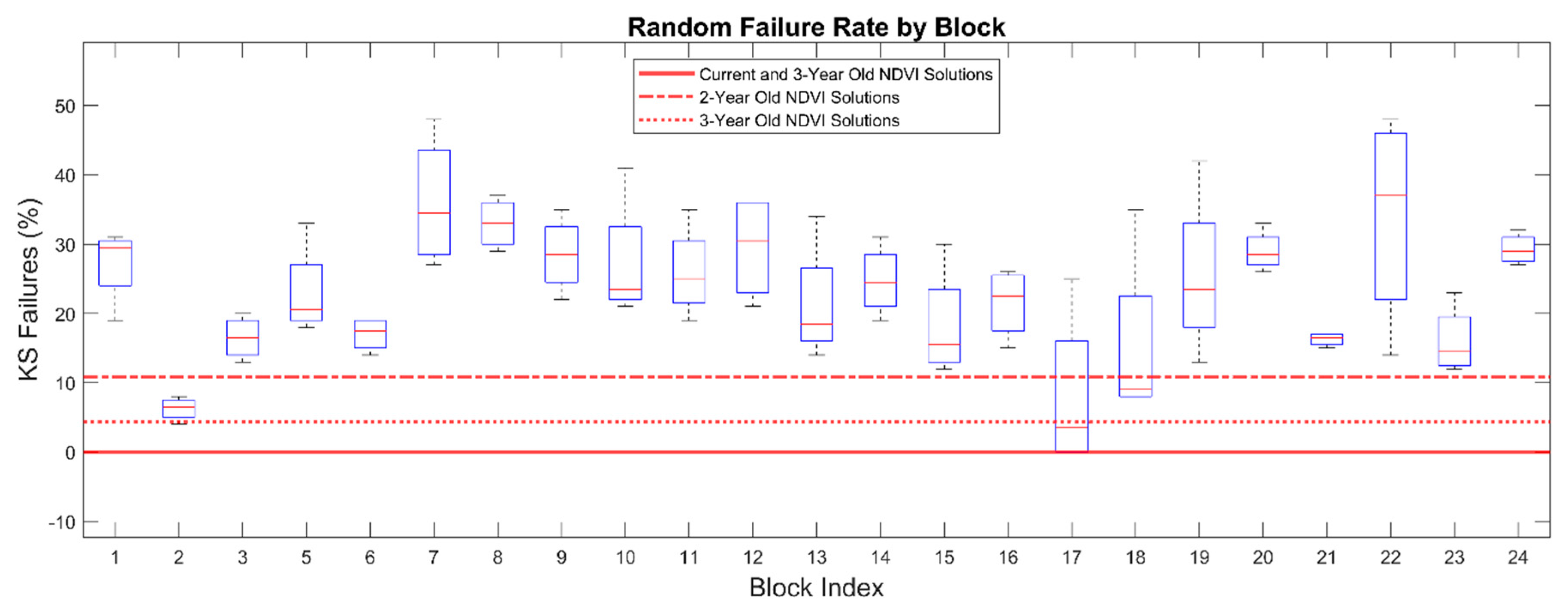
In a subsequent test, when three contiguous pixels were chosen at random, rather than optimized using the NDVI3 algorithm, K-S failure rates ranged from 0% to 50% with a mean of 23% (
Figure 3, right). The block-level K-S failure rate for random pixel selection is shown in
Figure 5.
4. Discussion
This work demonstrated that sampling the studied vineyards at a single location, as determined by the NDVI3 sampling protocol, resulted in more accurate sampling in many blocks compared to R20 and CM8. Operational efficiency (i.e., reduction in sampling time, reduction in distance travelled for sampling in a block) was not quantified in this study but was presumably increased due to the ability of vineyard staff to visit only a single location within the block to collect the required sample rather than traverse multiple vine rows.
It should be noted that all blocks in this study were uniform in soil type, drip irrigated, and receive very little natural rainfall compared to many other wine growing regions. For that reason, they are expected to be more uniform than vineyard blocks in most other wine growing regions. Variations in soil electroconductivity have been correlated with variations in NDVI response [
16] and increased soil variability within a vineyard could decrease the efficacy of NDVI3 sampling, perhaps required sampling protocols that cover more than three pixels to compensate.
The industry partners involved in this study use NDVI data from Landsat 7 to guide practices, hence it was used as the image source for the sampling solutions presented here. Presumably, these sampling solutions could be applied to remote sensing data of higher resolution (e.g., Sentinel-2) or spatial data from other sources (e.g., high resolution yield maps) although the solutions would need to be tested. Additionally, exploitation of spectral capabilities of remote sensing tools may provide greater accuracy and precision to these methods [
17].
The sampling solutions presented for the vineyards studied here were temporally stable. Once an NDVI3 solution was calculated for a block, it generally continued to pass the K-S test suggesting it would remain useful for several years, similar to the findings of [
18]. The 0% K-S failure rates for the longest time differentials (i.e., current to three-year-old solutions) seems likely coincidental, although it could suggest that spatial structure within the blocks has a seasonal pattern that oscillates over a multiyear period. Additional operational efficiency could potentially be gained by vineyards if new solutions only need to be recalculated occasionally rather than each season. The temporal stability of sampling solutions would likely be reduced in vineyards with more spatial and temporal variability such as those found in the cool climate region of the Northeastern U.S.
Potential areas of study for further improvement and refinement of spatially explicit sampling methods for monitoring fruit maturity include studying the efficacy in regions of higher soil and weather variability as well as analyzing satellite imagery of blocks in clusters to eliminate entire blocks from sampling. In the latter case, calibration of image clusters would be required to obtain a valid NDVI pixel population, but has the potential for substantially reducing labor through the elimination of visits and/or choosing sites to cluster based on shortest path of travel.
5. Conclusions
This work reports on a novel approach to grape sampling in a vineyard based on images obtained via remote sensing. The NDVI3 sampling protocol for grape maturation is functionally equivalent to or better than both R20 and CM8 in its ability to accurately estimate population Brix, TA, pH, and total anthocyanins of large, uniform vineyard blocks. The Kolomogorov-Smirnov test for population distribution of the samples indicated that the NDVI3 sample produced a p-value >0.90 for 12 of 13 blocks, while the R20 method produced a p-value of >0.90 for only 1 of 13 blocks. The commercial method currently used to sample these blocks (CM8) produced a p-value of <0.05 for 3 of 13 blocks.
Because NDVI3 sampling requires that a field technician locate and visit only one location within a block, rather than four for CM8 or 20 for R20, it would require substantially less time for vineyard staff to perform. The demonstrated temporal stability of NDVI3 solutions suggests that optimal solutions do not need to be computed for each season in Central Valley vineyards and that block spatial patterns are persistent across multiple seasons. Using NDVI images that were up to four years old resulted in a p-value of <0.05 for the Kolomogorov-Smirnov test in a maximum 11% of blocks.
The NDVI3 protocol has the potential to vastly improve the efficiency of sampling in Central Valley vineyards. However, vineyards grown in regions with more spatial and season-to-season variability than the studied vineyards could decrease the efficacy of NDVI3 sampling, perhaps required sampling protocols that cover more than three pixels.
The results of this study suggest that remote sensing and/or other spatial images warrant further investigation in their usefulness for guiding sampling in agricultural production systems.
Author Contributions
Conceptualization, J.M.M., N.D., C.R. and J.E.V.H.; Data curation, J.M.M., C.R. and C.B.; Formal analysis, J.M.M., C.R.; Funding acquisition, N.D. and J.E.V.H.; Investigation, J.M.M., C.R. and C.B.; Methodology, J.M.M., N.D., C.R., C.B. and J.E.V.H.; Project administration, N.D. and J.E.V.H.; Resources, N.D. and J.E.V.H.; Software Programming, J.M.M.; Supervision, N.D. and J.E.V.H.; Validation, J.M.M., N.D., C.R., C.B. and J.E.V.H.; Visualization, J.M.M.; Writing—original draft, J.M.M. and J.E.V.H.; Writing—review & editing, J.M.M., N.D., C.R., C.B. and J.E.V.H. All authors have read and agreed to the published version of the manuscript.
Funding
This research received no external funding.
Acknowledgments
This work was partially supported by a gift to the Vanden Heuvel research program at Cornell University from E.&J. Gallo Winery.
Conflicts of Interest
The authors declare no conflict of interest.
References
- Bramley, R.G.V.; Hamilton, R.P. Understanding variability in wine grape production systems 1. Within-vineyard variation in yield over several vintages. Aust. J. Grape Wine Res. 2004, 10, 32–45. [Google Scholar] [CrossRef]
- Meyers, J.M.; Vanden Heuvel, J.E. Use of normalized difference vegetation index images to optimize vineyard sampling protocols. Am. J. Enol. Vitic. 2014, 65, 250–253. [Google Scholar] [CrossRef]
- Panten, K.; Bramley, R.G.V. Whole-of-block experimentation for evaluating a change to canopy management intended to enhance wine quality. Aust. J. Grape Wine Res. 2012, 18, 147–157. [Google Scholar] [CrossRef]
- Student. Comparison between balanced and random arrangements of field plots. Biometrika 1938, 29, 363–379. [Google Scholar] [CrossRef]
- Jeffreys, H. Random and systematic arrangements. Biometrika 1939, 31, 1–8. [Google Scholar] [CrossRef]
- Van Es, H.M.; Gomes, C.P.; Sellmann, M.; van Es, C.L. Spatially balanced complete block designs for field experiments. Geoderma 2007, 140, 346–352. [Google Scholar] [CrossRef]
- Casler, M.D. Blocking principles for biological experiments. Appl. Stat. Agric. Biol. Environ. Sci. 2018, 3, 53–72. [Google Scholar]
- Roessler, E.B.; Amerine, M.A. Studies on grape sampling. Am. J. Enol. Vitic. 1958, 9, 139–145. [Google Scholar]
- Rankine, B.C.; Cellier, K.M.; Boehm, E.W. Studies on grape variability and field sampling. Am. J. Enol. Vitic. 1962, 13, 58–72. [Google Scholar]
- Iland, P.; Bruer, N.; Ewart, A.; Markides, A.; Sitters, J. Monitoring the Winemaking Process from Grapes to Wine: Techniques and Concepts; Patrick Iland Wine Promotions, Pty Ltd.: Adelaide, Australia, 2014. [Google Scholar]
- Meyers, J.M.; Sacks, G.L.; van Es, H.M.; Vanden Heuvel, J.E. Improving vineyard sampling efficiency via dynamic spatially-explicit optimisation. Aust. J. Grape Wine Res. 2011, 17, 306–315. [Google Scholar] [CrossRef]
- Meyers, J.M.; Vanden Heuvel, J.E. Enhancing the precision and spatial acuity of point quadrat analyses via calibrated exposure mapping. Am. J. Enol. Vitic. 2008, 59, 424–431. [Google Scholar]
- Ziliak, S.T. Balanced versus randomized field experiments in economics: Why W. S. Gosset aka ‘Student’ matters. Rev. Behav. Econ. 2014, 1, 167–208. [Google Scholar] [CrossRef]
- Krstic, M.P.; Leamon, K.; DeGaris, K.; Whiting, J.; McCarthy, M.; Clingeleffer, P. Sampling for wine grape quality parameters in the vineyard: Variability and post-harvest issues. In Proceedings of the 11th Australian Wine Industry Technical Conference, Adelaide, Australia, 11 October 2001. [Google Scholar]
- Stephens, M.A. Introduction to Kolmogorov (1933) On the Empirical Determination of a Distribution. In Breakthroughs in Statistics; Springer Series in Statistics (Perspectives in Statistics); Kotz, S., Johnson, N.L., Eds.; Springer: New York, NY, USA, 1933. [Google Scholar]
- Andre, F.; van Leeuwen, C.; Saussez, S.; Van Durmen, R.; Bogaert, P.; Moghadas, D.; de Resseguier, L.; Delvaux, B.; Vereecken, H.; Lambot, S. High-resolution imaging of a vineyard in south of France using ground-penetrating radar, electromagnetic induction and electrical resistivity tomography. J. Appl. Geophys. 2012, 78, 113–122. [Google Scholar] [CrossRef]
- Richter, K.; Tobias, B.H.; Vuolo, F.; Mauser, W.; D’Urso, G. Optimal exploitation of the sentinel-2 spectral capabilities for crop leaf area index mapping. Remote Sens. 2012, 4, 561–582. [Google Scholar] [CrossRef]
- Kazmierski, M.; Glémas, P.; Rousseau, J.; Tisseyre, B. Temporal stability of within-field patterns of NDVI in non irrigated Mediterranean vineyards. OENO One 2011, 45, 61–73. [Google Scholar] [CrossRef]
Figure 1.
Illustration of three-pixel normalized difference vegetation index (NDVI) directed sampling method. Dashed arrow represents path of travel during sampling. ‘X’s denote that sampling does not include vines from nearby pixels. Note that the path of travel is always limited to a single vineyard row and pixel orientation will differ from row orientation for rows that are not planted ether North-South or East–West.
Figure 2.
Illustration of three-pixel normalized difference vegetation index (NDVI) directed sampling method when row orientation is not North–South or East–West. Dashed arrow represents pat of travel during sampling. ‘X’s denote that sampling does include vines from nearby pixels. Note that the path of travel is always limited to a single vineyard row.
Figure 3.
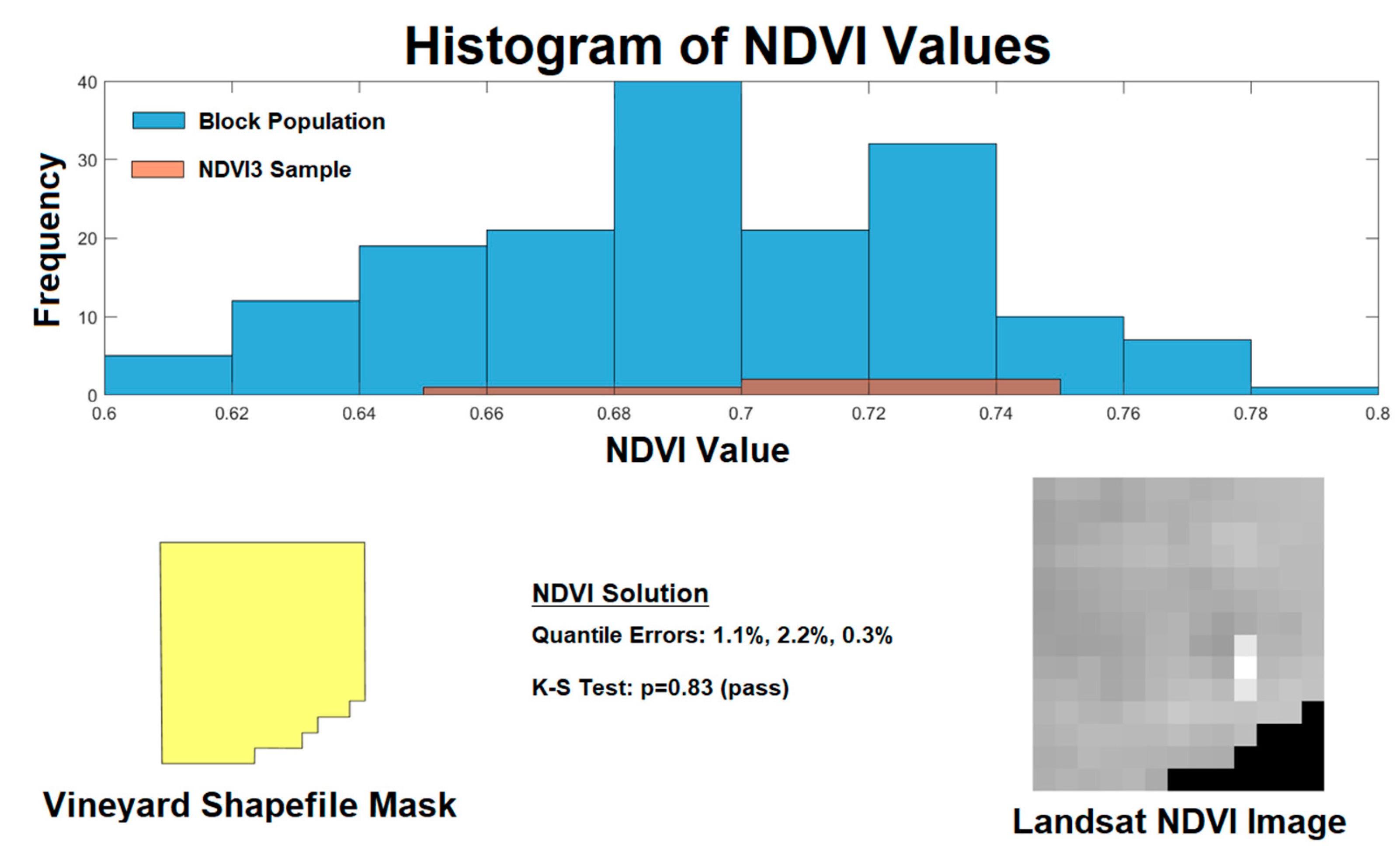
Example of Landsat image processing for evaluation of sample fitness. A shapefile (lower left) defines the boundaries of the vineyard which is used to acquire Landsat normalized difference vegetation index (NDVI) image (lower right). The highlighted area in the NDVI image represents the calculated NDVI3 sampling location. The histogram (top) demonstrates the population NDVI pixel values (blue) compared to the three pixels in the NDVI3 sample (orange). The quantile errors and Kolmogorov-Smirnov results are shown (lower center).
Figure 3.
Example of Landsat image processing for evaluation of sample fitness. A shapefile (lower left) defines the boundaries of the vineyard which is used to acquire Landsat normalized difference vegetation index (NDVI) image (lower right). The highlighted area in the NDVI image represents the calculated NDVI3 sampling location. The histogram (top) demonstrates the population NDVI pixel values (blue) compared to the three pixels in the NDVI3 sample (orange). The quantile errors and Kolmogorov-Smirnov results are shown (lower center).
Figure 4.
Kolmogorov-Smirnov test failure rates for NDVI-directed solutions (NDVI3) applied to Landsat normalized difference vegetation index (NDVI) imagery from multiple years. Left: solutions of age 0 are based on the previous season imagery and are the current solution. Negative ages indicate applying an old NDVI3 solution to imagery in future seasons. Positive ages indicate applying a new NDVI3 solution to previous season imagery. Right: failure rate of all blocks when three consecutive pixels are chosen at random rather than optimized with the NDVI3 algorithm.
Figure 5.
Block level Kolmogorov-Smirnov test failure rates of all blocks when three consecutive pixels are chosen at random rather than optimized with the NDVI3 algorithm.
Figure 5.
Block level Kolmogorov-Smirnov test failure rates of all blocks when three consecutive pixels are chosen at random rather than optimized with the NDVI3 algorithm.
Table 1.
Experimental vineyard blocks located in the Central Valley of California. Pixel counts are number of 30 x 30 m Landsat NDVI pixels analyzed. CS = Cabernet Sauvignon, C = Chardonnay, M = Merlot, PN = Pinot Noir, S = Symphony, Z = Zinfandel. Sampling using a three-pixel NDVI directed protocol (NDVI3) and eight-pixel quadrant directed protocol (CM8) methods was performed at 7-day intervals beginning on ‘Start Date’ and ending on ‘End Date’. Random sampling (R20) was performed once in 2016 at pre-harvest (R20-1) and twice in 2017 at veraison and pre-harvest (R20-1 and R20-2, respectively).
| Block ID | Pixels | Imaged Acres | Cultivar | Start Date | Stop Date | R20-1 | R20-2 |
|---|
| 2016-01 | 468 | 104.05 | C | 3 August | 24 August | 24 August | - |
| 2016-02 | 690 | 153.41 | C | 11 August | 29 August | 29 August | - |
| 2016-03 | 381 | 84.71 | C | 18 August | 29 August | 29 August | - |
| 2016-04 | 108 | 24.01 | CS | 21 August | 2 October | 2 October | - |
| 2016-05 | 291 | 64.70 | S | 18 August | 25 August | 25 August | - |
| 2016-06 | 729 | 162.08 | PN | 21 August | 4 September | 4 September | - |
| 2016-07 | 336 | 74.71 | M | 12 August | 2 October | 30 September | - |
| 2016-08 | 87 | 19.34 | CS | 17 August | 30 September | 2 October | - |
| 2016-09 | 396 | 88.05 | CS | 26 August | 2 October | 4 October | - |
| 2016-10 | 369 | 82.04 | C | 3 August | 10 August | 10 August | - |
| 2016-11 | 48 | 10.67 | Z | 31 August | 18 August | 18 August | - |
| 2016-12 | 291 | 64.70 | PN | 7 August | 11 September | 11 September | - |
| 2016-13 | 57 | 12.67 | CS | 19 August | 25 September | 26 September | - |
| 2017-01 | 165 | 36.69 | CS | 3 September | 25 September | 31 August | 25 September |
| 2017-02 | 56 | 12.45 | CS | 7 September | 8 October | - | - |
| 2017-03 | 55 | 12.23 | M | 25 August | 8 September | 31 August | 10 September |
| 2017-04 | 144 | 32.02 | CS | 14 September | 15 October | - | - |
| 2017-05 | 56 | 12.45 | M | 31 August | 14 September | 31 August | 14 September |
| 2017-06 | 50 | 11.12 | M | 29 August | 4 October | 29 August | 4 October |
| 2017-07 | 255 | 56.70 | M | 29 August | 4 October | 29 August | 4 October |
| 2017-08 | 167 | 37.13 | CS | 29 August | 12 October | 29 August | 12 October |
| 2017-09 | 312 | 69.37 | CS | 28 August | 16 October | 28 August | - |
| 2017-10 | 286 | 63.59 | M | 28 August | 16 October | 28 August | 9 October |
| 2017-11 | 272 | 60.48 | S | 28 August | 16 October | 28 August | - |
| 2017-12 | 240 | 53.36 | M | 28 August | 16 October | 28 August | 9 October |
| 2017-13 | 330 | 73.37 | M | 31 August | 11 October | 31 August | 11 October |
| 2017-14 | 84 | 18.68 | CS | 31 August | 26 September | 31 August | 26 September |
| 2017-15 | 176 | 39.13 | CS | 31 August | 5 October | 31 August | 5 October |
| 2017-16 | 156 | 34.68 | CS | 28 August | 16 October | 28 August | - |
| 2017-17 | 92 | 20.46 | CS | 31 August | 8 October | 31 August | 8 October |
| 2017-18 | 98 | 21.79 | CS | 7 September | 5 October t | - | - |
| 2017-19 | 214 | 47.58 | CS | 31 August | 26 September | - | - |
| 2017-20 | 156 | 34.68 | PN | 20 August | 1 September | 27 August | 1 September |
| 2017-21 | 249 | 55.36 | CS | 14 September | 15 October | - | - |
| 2017-22 | 57 | 12.67 | CS | 1 September | 22 September | - | - |
| 2017-23 | 50 | 11.12 | CS | 1 September | 19 September | - | - |
| 2017-24 | 428 | 95.16 | CS | 1 September | 22 September | - | - |
Table 2.
Overview of sampling methods used to sample vineyard blocks. Number of sampling locations refers to the number of predefined locations, expressed as GPS coordinates, sampled in each block. Number of pixels per location refers to the number of 30 × 30 m Landsat pixels traversed at each location during sampling. Pixels sampled is the product of locations and pixels per location. Number of clusters sampled totaled 20 per block for all methods.
| Treatment | Description | # Sampling Locations | # Pixels / Location | # Pixels Sampled | Total
# Clusters Sampled |
|---|
| R20 | Computer generated random pixel selection | 20 | 1 | 20 | 20 |
| CM8 | Four vineyards rows, one in each quadrant, sampled near end of row | 4 | 2 | 8 | 20 |
| NDVI3 | Three adjacent pixels representing the three quantiles of population | 1 | 3 | 3 | 20 |
Table 3.
Pearson correlation coefficients comparing fruit composition of samples collected via random sampling (R20), sampling using a three-pixel normalized difference vegetation index (NDVI) directed protocol (NDVI3), and sampling using an eight-pixel quadrant directed protocol (CM8) in vineyard blocks. R20 was performed once in 2016 (veraison) and twice in 2017 (veraison and pre-harvest). N = number of blocks sampled.
| Year | R20 Timing | Brix | TA | pH | Anthos |
|---|
| 2016 | | NDVI3 | CM8 | NDVI3 | CM8 | NDVI3 | CM8 | NDVI3 | CM8 |
| First (N = 13) | 0.85 | 0.89 | 0.91 | 0.93 | ND | ND | 0.98 | 0.91 |
| 2017 | First (N = 16) | 0.91 | 0.89 | 0.89 | 0.85 | 0.96 | 0.93 | 0.83 | 0.94 |
| Second (N = 16) | 0.73 | −0.05 | 0.90 | 0.78 | 0.98 | 0.95 | 0.95 | 0.88 |
| Combined (N = 32) | 0.93 | 0.86 | 0.96 | 0.93 | 0.98 | 0.96 | 0.90 | 0.90 |
Table 4.
Block statistics of normalized difference vegetation index (NDVI) pixel values, Kolomogorov-Smirnov (K-S) comparisons, and percentage of pixels sampled. Blocks were sorted by increasing block size. *A K-S p > 0.05 indicates that the sample is not considered to adequately represent the population.
| Block ID | Block Statistics (NDVI Value) | K-S Test p Value | % Pixels Sampled |
|---|
| Pixels | Acres | Min | Max | Mean | R20 | CM8 | NDVI3 | R20 | CM8 | NDVI3 |
|---|
| 2016-11 | 48 | 10.67 | 0.59 | 0.65 | 0.61 | 0.5591 | 0.0777 | 0.9773 | 41.7 | 16.7 | 6.3 |
| 2016-13 | 57 | 12.67 | 0.47 | 0.60 | 0.53 | 0.5259 | 0.8752 | 0.9934 | 35.1 | 14.0 | 5.3 |
| 2016-08 | 87 | 19.34 | 0.60 | 0.66 | 0.63 | 0.8659 | 0.3566 | 0.9080 | 23.0 | 9.2 | 3.4 |
| 2016-04 | 108 | 24.01 | 0.62 | 0.74 | 0.69 | 0.7899 | 0.0039* | 0.9450 | 18.5 | 7.4 | 2.8 |
| 2016-05 | 291 | 64.70 | 0.50 | 0.62 | 0.57 | 0.7241 | 0.1880 | 0.9515 | 6.9 | 2.7 | 1.0 |
| 2016-12 | 291 | 64.70 | 0.59 | 0.71 | 0.66 | 0.2537 | 0.9350 | 0.5179 | 6.9 | 2.7 | 1.0 |
| 2016-07 | 336 | 74.71 | 0.51 | 0.66 | 0.60 | 0.1895 | 0.0382* | 0.9794 | 6.0 | 2.4 | 0.9 |
| 2016-10 | 369 | 82.04 | 0.46 | 0.58 | 0.54 | 0.8151 | 0.7744 | 0.9987 | 5.4 | 2.2 | 0.8 |
| 2016-03 | 381 | 84.71 | 0.53 | 0.69 | 0.62 | 0.9944 | 0.2403 | 0.9664 | 5.2 | 2.1 | 0.8 |
| 2016-09 | 396 | 88.05 | 0.41 | 0.59 | 0.50 | 0.6312 | 0.0854 | 0.9484 | 5.1 | 2.0 | 0.8 |
| 2016-01 | 468 | 104.05 | 0.46 | 0.61 | 0.56 | 0.7445 | 0.0001* | 0.9043 | 4.3 | 1.7 | 0.6 |
| 2016-02 | 690 | 153.41 | 0.49 | 0.75 | 0.64 | 0.4574 | 0.2337 | 0.9994 | 2.9 | 1.2 | 0.4 |
| 2016-06 | 729 | 162.08 | 0.41 | 0.67 | 0.58 | 0.8679 | 0.1503 | 0.9522 | 2.7 | 1.1 | 0.4 |
© 2020 by the authors. Licensee MDPI, Basel, Switzerland. This article is an open access article distributed under the terms and conditions of the Creative Commons Attribution (CC BY) license (http://creativecommons.org/licenses/by/4.0/).

 ,
, 


