Article

Spectral Response Assessment of Moss-Dominated Biological Soil Crust Coverage Under Dry and Wet Conditions

1
Key Laboratory of Desert and Desertification, Northwest Institute of Eco-Environment and Resources, Chinese Academy of Sciences, Lanzhou 730000, China
2
University of Chinese Academy of Sciences, Beijing 100049, China
3
Arid Land Research Center, Tottori University, Tottori 680-0001, Japan
4
International Platform for Dryland Research and Education, Tottori University, Tottori 680-0001, Japan
*
Author to whom correspondence should be addressed.
Remote Sens. 2020, 12(7), 1158; https://doi.org/10.3390/rs12071158
Submission received: 18 March 2020 / Revised: 3 April 2020 / Accepted: 3 April 2020 / Published: 4 April 2020

Abstract

:
Biological soil crusts (BSCs) are a major functional vegetation unit, covering extensive parts of drylands worldwide. Therefore, several multispectral indices have been proposed to map the spatial distribution and coverage of BSCs. BSCs are composed of poikilohydric organisms, the activity of which is sensitive to water availability. However, studies on dry and wet BSCs have seldom considered the mixed coverage gradient that is representative of actual field conditions. In this study, in situ spectral data and photographs of 136 pairs of dry and wet plots were collected to determine the influence of moisture conditions on BSC coverage detection. Then, BSC spectral reflectance and continuum removal (CR) reflectance responses to wetting were analyzed. Finally, the responses of four commonly used indices (i.e., normalized difference vegetation index (NDVI); crust index (CI); biological soil crust index (BSCI); and band depth of absorption feature after CR in the red band, (BD_red)), calculated from in situ hyperspectral data resampled to two multispectral data channels (Landsat-8 and Sentinel-2), were compared in dry and wet conditions. The results indicate that: (i) on average, the estimated BSC coverage using red-green-blue (RGB) images is 14.98% higher in wet than in dry conditions (P < 0.001); (ii) CR reflectance features of wet BSCs are more obvious than those of dry BSCs in both red and red-edge bands; and (iii) NDVI, CI, and BSCI for BSC coverage of 0%–60% under dry and wet conditions are close to those of dry and wet bare sand, respectively. NDVI and BD_red cannot separate dead wood and BSC with low coverage. This study demonstrates that low-coverage moss-dominated BSC is not easily detected by the four indices. In the future, remote-sensing data obtained during the rainy season with red and red-edge bands should be considered to detect BSCs.

1. Introduction

Biological soil crusts (BSCs) consist of communities of living organisms (i.e., mosses, lichens, cyanobacteria, and liverworts) that exist within or directly on the surface of sand and soil [1,2]. Moss-dominated BSCs cover more than 10% of the land surface in some semi-arid areas of China [3]. BSCs are often described as ‘ecosystem engineers’ [4] because of their important role in carbon fixation [5,6], soil stabilization [1], and nitrogen budgets [6]. Due to the extreme vulnerability of BSCs to human activities and climate change, maintenance and preservation of BSCs should be a top management priority in arid regions [1,7]. Therefore, it is important to obtain accurate information on the spatial distribution and changes of BSCs so that the ecosystems can be evaluated and protected [8].
Multispectral and hyperspectral remote-sensing data have been used to investigate BSCs [9,10,11,12,13,14,15,16,17,18,19,20]. Many studies have focused on the identification of BSC spectral features [9,10,11,12,13,14,15]. The general spectral features of BSC include a chlorophyll absorption feature at a wavelength of approximately 680 nm [10,11,12,14,15,16,17]. Karnieli et al. [14] studied the spectral reflectance of moss-dominated BSCs and determined the differences between the spectra of vascular plants and bare sand. Karnieli [9] proposed the crust index (CI), and Chen et al. [10] proposed the biological soil crust index (BSCI) for use with multispectral satellite images in BSC detection. The CI uses the normalized difference between the blue and red bands, making it more appropriate to detect cyanobacteria-dominated BSCs [9], whereas the BSCI uses the red, green, and near-infrared (NIR) bands, which can better detect lichen-dominated BSCs [10]. In addition, Burgheimer et al. [18] found that the normalized difference vegetation index (NDVI) was useful in demonstrating the potential magnitude and efficiency of BSC assimilation activity.
Using hyperspectral remote-sensing data, continuum removal crust identification algorithm (CRCIA) [12], crust development index (CDI) [11], and a rule based on support vector machine (SVM) and spectral mixture analysis (SMA) [8] have been proposed for prediction of BSC distribution using continuum removal (CR) techniques. CR [21] is good at isolating particular, subtle absorption features for spectral analysis, and has been used to determine absorption peaks of BSC [8,22]. Although hyperspectral remote sensing of BSC performs better than multispectral remote sensing [19], lower data availability and higher calculation demands of hyperspectral data are critical constraints for its widespread use [17,20]. In addition, satisfactory results for detecting BSC cannot be obtained when applying common vegetation indices [12,17,23]. Therefore, it is important to study more deeply the use of multispectral remote sensing to monitor BSC. Based on this, Chen et al. [17] applied a random forest algorithm to multispectral data to estimate BSC distribution in Mu Us Sandy Land, and Panigada et al. [20] developed a new index using multi-temporal Sentinel-2 images to monitor BSC in the Negev Desert, Israel.
However, BSCs are very sensitive to wet and dry conditions because they consist of organisms referred to as poikilohydric [18,24,25]. Water scarcity restricts metabolic activity of BSCs, whereas water availability facilitates photosynthesis [25,26]. Fang et al. [25] studied spectral variations in dry and wet moss soil crust in July and September. They found that the CI and BSCI values of wet moss soil crust were similar to those of Artemisia ordosica both in summer and fall [25]. Karnieli et al. [27] conducted BSC-wetting experiments, which indicated that in both the visible and infrared ranges, progressive increases in physiological activities result in decreases in reflectance. They also found an increase of NDVI values in BSCs after wetting, unlikely to be related to changes in soil spectral features but rather to the photosynthesis process of BSC organisms. Rodríguez-Caballero et al. [28] came to a similar conclusion, finding that NDVI values strongly increased with BSC wetness. They reported a decrease of reflectance between 450–900 nm and a long-term effect on the spectral features of BSC after wetting. O’Neill [15] observed a deepening of the absorption feature and a shift in red and red-edge bands after 10 minutes wetting of BSC. CR has also been used to detect changes in subtle spectral features of BSCs between dry and wet conditions [20,22,29,30]. Escribano et al. [22] used CR to differentiate between BSC growing in spring and summer. Based on CR reflectance at 680 nm and its response to dry and wet conditions, Blanco-Sacristán et al. [29] established a spectral diversity metric to track spatiotemporal changes in lichen-dominated BSCs. Román et al. [30] focused on using CR to quantify chlorophyll-a concentration (Chla) of BSC, and found that NDVI is also sensitive to changes in BSC Chla, although NDVI was not as accurate as CR. Panigada et al. [20] reported that Chla absorption depth calculated by applying CR to multispectral data (BD_red), can reflect the greening of BSC after wetting but not the soil moisture content. On this basis, they proposed indices according to the time difference to detect BSC (before and after the first rain) and vegetation (before and after the whole rainy season). Additionally, Lehnert [23] found that the water absorption feature at 1420 nm reacts much stronger for photosynthetic activity of BSC than the chlorophyll absorption bands. However, these dry-wet studies have used pure BSC plots or plots with >90% BSC coverage, which are relatively rare in the field. Therefore, these results are not applicable as a reference for multispectral remote-sensing detection of BSCs. Further studies are needed on dry and wet BSCs with a mixed coverage range representative of actual field conditions.
This study aimed to provide a better understanding of multispectral remote-sensing data and technique selection, as well as detection conditions for BSC estimation by remote sensing to ensure accurate detection of BSCs. The specific objectives of this study were to: (i) determine the influence of dry and wet conditions on the estimation of BSC coverage using RGB images; (ii) determine the spectral and CR spectral responses of BSCs to dry and wet conditions within different coverage levels; and (iii) evaluate the response of four commonly used vegetation and BSC indices (NDVI, CI, BSCI, and BD_red) calculated using two multispectral data bands (Landsat-8 and Sentinel-2) to dry and wet conditions with different BSC coverage levels.

2. Materials and Methods

2.1. Study Area

This study was conducted in the Mu Us Sandy Land in northern China (37°28′–39°49′ N, 106°57′–110°37′ E). The Mu Us Sandy Land covers an area of approximately 4 × 10⁴ km2 and is located at an altitude of 875–1685 m (Figure 1). The annual average temperature is between 6.0 ℃ and 8.5 ℃ [31]. Rainfall mainly occurs between July and September (particularly in August), accounting for 60%–75% of total annual precipitation. The average potential annual evaporation in this period is 2300 mm, which is six times the annual average precipitation. The soil type is loose eolian sandy soil, which is infertile and vulnerable to wind erosion [17]. After thousands of years of human activities (such as reclamation of farmlands, deforestation, and overgrazing), natural vegetation in the sandy land has almost disappeared. Most of the existing vegetation has been artificially planted. Over 80% of the sandy areas are covered by sandy grassland [32,33]. The dominant species is A. ordosica [32]. Other main vegetation species on the sandy grassland are Stipa glareosa, Artemisia frigida, Achnatherum splendens, Suaeda glauca, and Kalidium foliatum. Moss-dominated BSC exists widely in the A. ordosica community and plays a key role in sand dune fixation [32,34]. The dominant species and common species of cyanobacteria, lichen, and moss in Mu Us Sandy Land are shown in Table 1. The Mu Us Sandy Land has a semi-arid continental climate, which is sensitive to changes in land use and climate [33].

2.2. Datasets

2.2.1. Field Spectra Measurement and Classification of Plots

A field survey was conducted between 28 June and 4 July 2017; a portable spectrometer (Field Spec Handheld2, ASD, Boulder, CO, USA) was used to measure the in situ spectral reflectance of 136 BSC plots (Figure 2a) classified as BSC (pure BSC plots, abbreviated as C, 42 replicates), BSC with plants (C+P, 28 replicates), BSC with dead wood (C+D, 47 replicates), and mixed (BSCs plots mixed with plants and dead wood, abbreviated as M, 19 replicates) (Figure 2e). In addition, the spectra of A. ordosica (69 replicates), dead wood (40 replicates), and bare sand (4 replicates for both dry and wet conditions) were measured. The portable spectrometer was used for the measurements at wavelength increments of 2 nm within a 325–1075 nm range, with a 15 ° field of view (FOV), and at a height of approximately 1 m above the ground. Spectral measurements were carried out under bright and sunny conditions from 10:00 to 15:00 China standard time (UTC+8) [17].

2.2.2. Pairwise Dry and Wet Biological Soil Crust (BSC) Field Plots

A metal hoop with a 26 cm diameter (Figure 2b) was constructed to ensure that each plot covered 100% of the FOV of the portable spectrometer sensor. A reference wet condition was established by spraying 200 mL of water in the hoop and waiting for water to seep for 1 minute (Figure 2a). The metal hoops were only used when the photographs were taken (described in 2.2.3) and to mark out the area for watering; they have been removed during the field spectra measurements (described in Section 2.2.1). The amount of water (200 mL) used to wet the plots is related to rainfall in Mu Us Sandy Land. The maximum value of average daily precipitation from 1961 to 2016 in the eastern region of Mu Us Sandy Land is 5.68 mm, in the central region is 4.70 mm, and in the western region is approximately 3.47 mm. We assume precipitation of moderate to heavy rainfall in Mu Us Sandy Land is 3.7 mm, and the amount of water required to simulate such rainfall in the area enclosed by the metal hoop is approximately 200 mL. According to Rajeev et al. [35] and Proctor and Smirnoff [36], the greening of moss-dominated crusts increases within 3 minutes after wetting, and the recovery of their photosystems takes around 10–20 minutes. Therefore, the BSC coverage data (estimation method described in Section 2.2.3) in wet conditions were collected approximately 3–4 minutes after wetting. In situ spectral data in wet conditions were collected approximately 8–10 minutes after wetting. Dry conditions were defined as natural conditions on a sunny day, with no immediate treatment. The soil samples were collected during the field survey to determine soil water content in dry and wet conditions. The average soil moisture content at a depth of 0–10 cm in dry conditions is 4.80%. After spraying with water, the average moisture content increased from 2.36% to 7.16%. The increased soil moisture content accounts for 49.21% of the dry plots. The water content of soil (WC) was determined by the drying method [37]. Briefly, the wet weight of the soil sample is referred as WM and the dry weight as DM. The weight of the aluminum box was recorded as m. The soil moisture content was calculated using Equation (1), and the increase in soil moisture content was calculated using Equation (2):
WC (%) = (WMDM)/(DMm) × 100%
WC (increase %) = [WC (wet) − WC (dry)]/WC (dry) × 100%

2.2.3. Estimation of BSC Coverage

The BSC coverage was estimated as described by Chen et al. [17]. Photographs were taken of the BSCs in the hoop (D3000 digital camera, Nikon) (Figure 2b), after which Adobe Photoshop CC (19.1.6) and CAN_EYE (v 6.491) software were used to clip the hoop area and determine the BSC coverage (Figure 2c,d). CAN_EYE could only separate two elements. One element is defined as BSCs; another is defined as a mixture of sand, vegetation, and dead wood in the software. Masks were created in CAN_EYE to exclude some mixed pixels that had very similar colors to BSCs or sand.

2.3. Treatment of Spectral Datasets

Ten spectra were determined at each plot and mean values were entered into a Microsoft Excel 2016 (16.0.12228.20100) worksheet as final reflectance spectra.

2.3.1. Continuum Removal (CR)

A CR algorithm was applied to spectra from plots within different cover types [38]. The continuum is a convex ‘hull’ of line segments fitted along the top of the spectra to connect the local spectral maxima and represent the baseline [21]. This algorithm enhances absorption features and distinguishes them [21,38,39]. This treatment was conducted using ENVI 5.3 software.

2.3.2. Hyperspectral Resampling

To simulate real remote-sensing datasets, in situ spectral data were first resampled by using the spectral response functions (Figure 3) [40,41] of the multispectral Landsat-8 and Sentinel-2 channels (Table 2). Given that the hyperspectral wavelength ranges of 325–400 nm and 900–1075 nm were severely affected by noise, only the range 400–900 nm was accounted for when resampling.

2.3.3. Index Calculations

NDVI [42], two BSC indices (CI and BSCI) [9,10], and BD_red [20] were calculated to determine responses to dry and wet conditions (Equations (3)–(6)):
NDVI = ( R NIR R Red ) / ( R NIR + R Red )
CI = 1 ( R Red R Blue ) / ( R Red + R Blue )
BSCI = ( 1 L × | R Red R Green | ) / R Green   Red   NIR mean
BD _ red = 1 CR _ red
In these equations, R is the reflectance value in the NIR, red, blue, and green bands. Based on observations by Chen et al. [10], L was set to 2 as an adjustment parameter to amplify the absolute difference between RRed and RGreen. CR-red is the reflectance values after CR in the red band.

2.4. Statistical Analysis

Paired double-sample t-test analyses were performed on BSC coverage and spectral indices using Microsoft Excel 2016 for comparison under dry and wet conditions (Figure 4). The above study process has three aims, as shown in Figure 4.

3. Results

3.1. Influence of Dry and Wet Conditions on BSC Coverage Estimation

Figure 5a illustrates BSC coverage estimation from one pair of plots (out of 136 pairs). The estimated BSC coverage increases significantly after the plots were sprayed with water, regardless of land-cover type (Figure 5; Figure S1). Estimations of wet BSC coverage increase by 14.82%, 17.91%, 10.12%, and 17.00% compared with those of dry BSC coverage in the C, C+P, C+D, and M cover types, respectively. However, five points that were covered with biocrust and dead woods (C+D) exhibit higher BSC coverage in dry conditions than in wet conditions (Figure 5c, red points; Figure S1c). Plots with 0% dry BSC coverage remain at 0% in wet conditions (Figure 5c, orange points; Figure S1a).

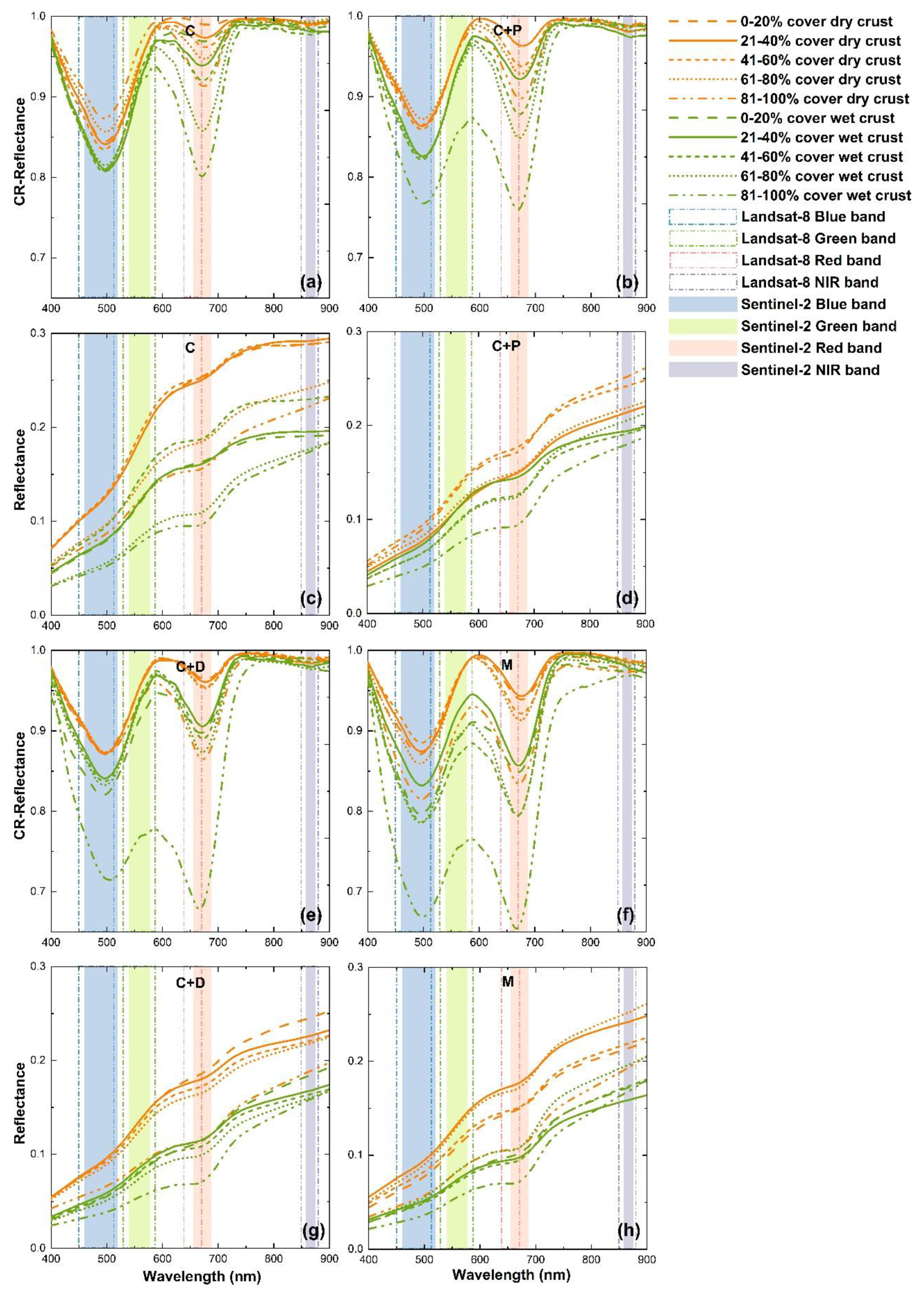
3.2. Response of BSC Spectrum to Dry and Wet Conditions

As every plot had two BSC coverage values (dry and wet), wet BSC coverage represented the metabolic-activated BSC. BSC coverage data in the dry conditions was not involved in spectral analysis. In general, spectral reflectance of dry BSC plots are higher than those of wet BSC plots (Figure 6 and Figure 7, Table S1); the higher the BSC coverage area, the lower the reflectance (Figure 6). After CR processing, absorption features in the blue and red bands became more prominent (Figure 6 and Figure 7). Apart from differences in reflectance values, there are no other spectral features exhibiting substantial differences between the different cover types (C, C+P, C+D, M) (Figure 6 and Figure 7).
C-type wet BSC plots within all coverage ranges, and C+P, C+D wet BSC plots within 0%–80% coverage ranges show almost the same absorption values of CR reflectance in the blue band (Figure 6a,b,e). In the red band, the CR absorption features of type C+P are slightly higher than those of type C (Figure 6a vs. Figure 6b). The CR absorption features of 80%–100% cover BSC in type C+D and type M plots were much more obvious than in type C and C+P plots (Figure 6a,b vs. Figure 6e,f). The C-type BSC coverage ranges of 0%–20%, 60%–80%, and 80%–100% show significant differences between dry and wet conditions in all bands (P < 0.001) (Table S1). In general, for C-type BSC plots with 80%–100% coverage, the dry BSC spectra are 41.10% higher than those of wet BSC in the Coastal Aerosol band, and 40.38%, 37.63%, 38.55%, 27.88%, and 21.73% higher in the blue, green, red, red-edge, and NIR bands, respectively (Table S1).
Average 400–900 nm reflectance is greatest in bare sand, followed by type C+P, C, C+D BSCs, and smallest in M-type BSCs, in both dry and wet conditions (Figure 7a). Although bare sand has the highest reflectance, Figure 7b shows that the absorption features in the blue band of bare sand are very similar to those of dry BSCs. However, dry and wet bare sand curves are almost horizontal in the red and red-edge bands after CR whereas BSCs exhibit absorption and reflection features, especially in wet conditions (Figure 7b). The absorption features of dead wood in the red band are almost identical to those of all types of BSCs within 20%–80% coverage in dry conditions (CR_red ≈ 0.95) (Figure 6a,b,e,f and Figure 7b). A. ordosica shows clear absorption in the blue and red bands (Figure 7a), and reflection in the green band. The BSC reflectance features in the green band were greater than those of A. ordosica.

3.3. Normalized Difference Vegetation Index (NDVI), Crust Index (CI), Biological Soil Crust Index (BSCI), and Band Depth of Absorption Feature after Continuum Removal in the Red Band (BD_red) of BSCs with Different Coverage Ranges in Dry and Wet Conditions

Type C plots were used to calculate four indices of pure BSCs with different coverage ranges in dry and wet conditions (Figure 8). Unlike for NDVI and BD_red, no significant differences were observed in the CI and BSCI between dry and wet conditions in the 40%–60% coverage range. These four indices of BSCs calculated from Landsat-8 and the Sentinel-2 bands show identical trends in dry and wet conditions (Figure 8a vs. Figure 8b, Figure 8c vs. Figure 8d, Figure 8e vs. Figure 8f, Figure 8g vs. Figure 8h).
After wetting, NDVI values for all coverage ranges increased significantly (Figure 8a,b). As the BSC coverage area increases, differences in NDVI values between dry and wet conditions also increase. For C-type covering 80%–100% of the plot, the NDVI value for wet BSC is 59.29% higher than that of dry BSC. The NDVIs of 0%–20% coverage areas under both dry and wet conditions are almost identical to those of bare soil (Figure 8a,b). Figure 7a,b show that the NDVI value of A. ordosica is much higher than that of BSCs with different coverage values. Furthermore, the NDVI value of dead wood is close to that of 60%–80% coverage with dry BSCs.
In contrast, Figure 8e,f show that the CI value decreases after water spraying and is less sensitive than the other two indices. On average, the CI value of wet BSC is 2.3% lower than that of dry BSC. There is no significant difference between the CI values in dry and wet conditions within the BSC coverage range of 0%–60%. When the BSC coverage increases, the CI value increases slowly. It is easy to distinguish dead wood and A. ordosica, for which the CI values are higher than those of BSCs with different coverage levels (Figure 8c,d). However, for the CI calculated using Landsat-8 bands, the values in dry and wet bare sand are almost equal to those of 0%–20%, 20%–40%, and 40%–60% coverage with dry and wet BSCs (Figure 8c). In contrast, the CIs of dry and wet bare soil calculated using the Sentinel-2 bands are lower than those of all coverage values for dry and wet BSCs (Figure 8d).
The BSCI values show almost the same trend as the NDVI values (Figure 8a vs. Figure 8e, Figure 8b vs. Figure 8f). The BSCI values for 40%–60% coverage BSCs show no significant difference between dry and wet conditions (Figure 8e,f). In contrast to the NDVI, the BSCI of dead wood is the highest and is distinguishable (Figure 8e,f). The BSCI values of A. ordosica, 0%–40% coverage of wet BSCs, and wet bare sand are similar (Figure 8e,f). Furthermore, the BSCI values of dry bare sand and of 0%–60% coverage dry BSCs are relatively close.
For BD_red, there are significant differences (P < 0.01) of BSC between dry and wet conditions for all coverage ranges (Figure 8g,h). With the increase of BSC coverage, the BD_red values of BSC increase gradually, irrespective of whether the conditions were dry or wet. Like NDVI, the BD_red of A. ordosica (BD_red = 0.7367) is much higher than that of BSC (BD_red <0.3), bare sand (BD_red <0.02) and dead wood (BD_red = 0.0378).

4. Discussion

4.1. Influence of Dry and Wet Conditions on BSC Coverage Estimation

One of the reasons that most of the estimates of BSC coverage in wet conditions are higher than in dry conditions is because the leaves of bryophytes can rehydrate and become fully expanded in wet conditions [1,24,28]. This is considered to be the desiccation tolerance of BSCs [43,44]. After wetting, photosynthesis, cell infiltration, and cell structure of BSCs recover rapidly [43,45]. Another explanation for this observation might be related to the misclassification of dry BSC into sand or soil due to the similar color of them. Only type C+D shows smaller BSC coverage in wet plots than in dry plots. This may be because the spectral absorption features of dry BSCs are nearly the same as those of dead wood (Figure 7b). This could lead to classification errors in dry conditions. After spraying with water, the absorption features were enhanced [15,24,27,28], making it easier to identify BSCs and dead wood. Bare sand (i.e., 0% BSC coverage) shows no difference in coverage areas between wet and dry conditions (Figure 5c, orange points; Figure S1a), which means that dark-colored bare sand in wet conditions will not be mistaken for BSCs. Therefore, the influence of soil moisture condition on BSC coverage might be overestimated (Figure 5a). This means RGB images cannot estimate BSC accurately in dry conditions. The significant differences in BSC coverage estimation between dry and wet conditions highlight the importance of identifying spectral changes in dry and wet conditions to determine more spectral bands for BSC estimation. In order to avoid the influence of misclassification in the spectral analysis, we used BSC coverage data in the wet conditions and divided coverage into five levels (0%–20%, 20%–40%, 40%–60%, 60%–80%, and 80%–100%), which could greatly reduce the error rate of BSC coverage classification.

4.2. Response of BSC Spectra to Dry and Wet Conditions

The reflectance of dry BSCs is higher than that of wet BSCs for all cover types, which is consistent with many studies [14,15,25,46]. When soil moisture increases, the decrease in reflectance leads to a decrease in brightness [47], which affects the coverage estimation from digital photos (Figure 5a). Type C, C+P, C+D, and M covers did not appear to have different spectral absorption features, but only different reflectance values (Figure 7). This demonstrates that, in this study area, BSCs with different cover types and areas can have unified spectral features. No significant difference of 40%–60% BSC between dry and wet conditions were observed in the green, red, red-edge, and NIR bands (P > 0.05) (Table S1). This may be because the plots with mid-range BSC coverage could consist of light-colored chlorolichens (e.g., Diploschistes muscorum, see Table 1, Figure S2) [48]. In the blue band, CR reflectance values of type C, C+P, and C+D plots within 0%–80% BSC cover were almost identical, which indicates that the absorption features in the red band are more important for detecting changes in BSC coverage. Since red band absorption features are related to Chla content of BSCs, several researchers [20,22,29,30] have used CR reflectance values in the red band to study BSCs in dry and wet conditions. Panigada et al. [20] pointed out that CR reflectance in the red band could reflect the greening of BSCs after wetting but not the soil moisture content. In this study, the maximum responses in the red band to wetting happened in the mixed plots (type M) and BSC with dead wood plots (type C+D), but not in the pure plots (type C) (Figure 6a,b,e,f and Figure 7b). One possible reason for the maximum response in type M is that this cover type may have a higher proportion of vegetation since CR reflectance in the red band at the 80%–100% coverage level in dry conditions is lower than for the other levels. Another possible reason is that there will be a positive effect of greater water availability promoted by dead wood on BSC chlorophyll content [49]. In addition, C+D and M type plots contained some dead wood, which might indicate the existence of rich organic matter in the soil. Li et al. [34] reported that, at 0–3 cm of the soil surface, the soil organic matter exhibited the following order: moss soil crust (12.54 g kg−1) > lichen soil crust (6.81 g kg−1) > algae soil crust (4.27 g kg−1). Lan et al. [50] found that crust Chla generally increased with the development and succession of BSCs. Therefore, rich organic matter might lead to an abundance of chlorophyll concentration in BSCs, so that in the red band, cholorophyll absorption is more obvious. However, we do not have coverage data of each element (plants, dead wood, and different BSC species) in the plots. To produce a more accurate analysis, future research will focus on the proportion of each component in the plots.
In this study, BSCs in wet conditions are distinguishable from dead wood in the red and red-edge bands (Figure 6b). Moreover, wet BSCs show more obvious spectral features than bare sand in the red-edge bands (Figure 7b). Therefore, we assume that moss-dominated BSCs under wet conditions may be easily predicted. Spectral reflectance in Landsat-8 bands and Sentinel-2 bands in the 400–900 nm range show the same trends between dry and wet conditions (Table S1). Although the red and blue bands are considered to be effective bands for BSC prediction [9,16,20,29], clear data troughs (Figure 7b) for all BSC cover types in the 700–800 nm range, means that the data which have red-edge band can predict BSCs better than the data without the red-edge band. O’Neill [15] also found that BSCs have a shift in the red-edge band. Thus, the red-edge bands of Sentinel-2 data (see Figure 3, Table 2) could be more effective for BSC prediction than Landsat-8 data. In the green band, the reflection features of A. ordosica are found at approximately 550 nm, while the reflection features of both dry and wet BSC are at approximately 590 nm. We believe that this staggered reflection peak in the green band may be used to detect BSCs in future when better multispectral datasets become available.

4.3. NDVI, CI, BSCI, and BD_red of BSCs with Different Coverage Ranges in Dry and Wet Conditions

Regarding the NDVI, the higher the BSC coverage, the greater the difference between dry and wet conditions (Figure 8a,b). This may be due to increased chlorophyll activation in areas that are covered with more BSCs after being subjected to wet conditions [25,51]. Furthermore, the similarity of NDVI values for BSCs with 0%–20%, 20%–40%, and 40%–60% coverage might be due to the large proportion of bare sand in these plots. Weber and Hill [16] concluded that NDVI is sensitive to chlorophyll absorption features. However, it is not easy to distinguish BSCs using NDVI based on NDVI values of the soil (0.05–0.25) and sparse woody vegetation (0.1–0.15) [52]. This was also confirmed by our results: plots with 0%–60% coverage of BSCs contained more organisms with lower chlorophyll content (lichen and cyanobacteria) and mixed with a large proportion of sand meant that the NDVIs of the BSC cannot be distinguished from the range of NDVI values of bare sand (Figure 8a,b). That is why we can still observe that as the BSC coverage increases, the NDVI values of wet BSC also increase slightly (because of the increase of chlorophyll), while the NDVI values of dry BSC are basically the same as that of bare sand in dry conditions. The causes of a likely lower than expected chlorophyll concentration in wet conditions in the coverage range 40%–60% are still unknown, but it could be related to the BSC community composition. Although NDVI is sensitive to soil moisture content [53], the increase in NDVI values in our study between dry and wet bare sand (Figure 8a,b) is not significant. The possible reason might be that our simulated rainfall was 3.7 mm, which only increased soil moisture content by 2.36%. Therefore, the NDVI did not significantly increase, which is consistent with the results of Farrar [53].
Unlike NDVI, BSCI, and BD_red, CI values decrease after wetting, which could be because the blue and red bands are used for determining the CI. The CI is mainly used for the detection of cyanobacteria-dominated BSCs [9]. Cyanobacteria are involved in the initial stage of bryophyte crust development [48,54]; thus, the in situ plots must also have contained cyanobacteria. In dry conditions, the color saturation of cyanobacteria is higher than in wet conditions; therefore, the dissimilarity between red and blue bands in dry conditions is higher than in wet conditions [14]. The higher the reflectance value in the blue band is, the smaller the CI value is. However, according to Equation (4), the increase or decrease of reflectance value in the red band cannot determine the trend of CI value. This might result in the low differences between dry and wet conditions in the CI of low coverage BSC. The statistically significant differences in the highest coverage (80%–100%) of BSC might be due to a greater amount of cyanobacteria being integrated into the higher coverage of BSCs (Table S1). Fang et al. [25] found that CI values of moss soil crust (MSC) increased with increasing soil moisture. A possible reason for our contrasting results is the different wetting methodology between Fang et al. [25] and this study. The waiting time after wetting in our study may have been insufficient so that the increase in soil moisture content is lower than in Fang’s study [25]. This would prevent the absorption effects in the red band from reaching their peak. Other studies have shown a more pronounced curve in the red band for mosses using the CR technique [11,29]. This inadequacy of our research design can also explain why Fang et al. [25] showed that the spectral features of wet MSC are similar to those of A. ordosica, while our study did not. CI increased slowly with increases in the coverage level. This is consistent with Weber and Hill’s [55] conclusions, which indicate that CI fails to detect BSC abundance. Chen et al. [10] also mentioned that CI would be less suitable for BSCs where cyanobacteria are not the dominant constituent. However, the CI value can be used to distinguish BSC from A. ordosica and dead wood (Figure 8c,d). Weber and Hill [55] emphasized this good performance of CI to distinguish BSC from other ground objectives. Chen et al. [17] also noted that a combination of CI bands is better for BSC identification when using random forest algorithms to detect BSCs.
It should be noted that the BSCI value of BSCs with 40%–60% coverage was not sensitive to wetting (Figure 8e,f). This may be because of the presence of the light-colored chlorolichens mentioned in Section 4.2, which means that the reflectance values show no significant differences in the green, red, and NIR bands after wetting (see Table S1); the BSCI is calculated using these three bands. The CI and BSCI values of dead wood are high, meaning that dead wood can easily be distinguished using these two indices (Figure 8c–f). At 0%–60% coverage, NDVI, CI, and BSCI of dry and wet BSCs are close to those of dry and wet bare sand (Table S1, Figure 8). This indicates that when the coverage is lower than 60%, the three indices can hardly distinguish BSCs from bare sand. Chen et al. [10] also noted that the BSCI is not reliable when the BSC coverage is <33%. Another important limitation of the BSCI is that it must be applied under conditions where higher plants exhibit no photosynthetic activity [55], which is consistent with our results that the BSCI cannot easily distinguish A. ordosica from wet BSC with 0%–60% coverage (Figure 8e,f).
In Panigada’s research [20], BD_red can reflect the greening of BSC after wetting but not the soil moisture content. This is also reflected in Figure 8g,h that the similarity between dry and wet bare sand vs. the significant differences (P < 0.01) of BSC between dry and wet conditions. Román et al. reported that both NDVI and CR-red are sensitive to Chla in BSCs and CR-red is more sensitive. This is confirmed in our study. Compared with NDVI and BD_red, we found that the BD_red value was not easily affected by the sand base, but more accurately reflected the content of chlorophyll. It works well to discriminate BSC from sand in almost all BSC coverage ranges. However, like NDVI, BD_red cannot distinguish dead wood from BSCs within 20%–60% coverage in dry conditions (Figure 8g,h).

5. Conclusions

Based on our results, we conclude that changes in soil moisture will have a great impact on the estimation of biological soil crusts (BSCs). The misclassification of BSC in RGB images is inevitable in dry conditions. CR reflectance features of wet BSCs are more obvious than those of dry BSCs in both red and red-edge bands. We suggest that when using multispectral remote-sensing data to predict BSCs over a large area, data with red and red-edge bands should be used and estimations better made during the rainy season. Furthermore, low coverage moss-dominated BSC is not easily detected by the normalized difference vegetation index (NDVI), crust index (CI), and biological soil crust index (BSCI). Although the band depth of absorption feature after continuum removal in the red band (BD_red) is sensitive to the greening of BSC, it cannot distinguish low-coverage BSC from dead wood. Therefore, more bands (i.e., green, red-edge bands) and calculations or algorithms should be considered in future to detect BSC accurately. The analysis of spectral responses of moss-dominated BSC under dry and wet conditions will contribute to a better understanding of BSC detection by remote sensing.

Supplementary Materials

The following are available online at https://www.mdpi.com/2072-4292/12/7/1158/s1: Figure S1: Estimation of BSC coverage in dry and wet conditions with the cover of (a) C, (b) C+P, (c) C+D, and (d) M. A pair of yellow and green points on the same x-axis is one plot in dry and wet conditions respectively. All plots are arranged from low to high according to the BSC coverage under wet conditions. Figure S2: Photos of 40%–60% coverage biological soil crust (BSC) plots which contain light-colored lichens. Table S1: Reflectance response of the C cover type biological soil crusts (BSCs) in the Landsat-8 and Sentinel-2 bands under dry and wet conditions. Data are presented as means ± SE. Within each coverage group in each band, superscript “***” indicates a very large significant difference between the means under dry and wet conditions at P < 0.001; superscript “**” indicates a highly significant difference between the means under dry and wet conditions at P < 0.01; superscript “*” indicates a small, but significant difference between the means under dry and wet conditions at P < 0.05; and superscript “ns” indicates no significant difference between the means under dry and wet conditions at P > 0.05, based on the Excel-paired two-sample mean analysis results. See Table 2 for band details.

Author Contributions

T.W., A.T., S.L., X.C. and F.P. designed and supervised the study. S.L. and X.C. designed and performed the fieldwork, W.K., Z.G., and K.F. provided assistance during fieldwork. J.L. provided help during the data analysis. C.X. analyzed the data and drafted the manuscript. All authors read, revised, and approved the manuscript.

Funding

This work was supported by the Project of National Key Research and Development Program of China, “Assessment on evolution trend and stability of desertified land in the semi-arid region of northern China” [grant number 2016YFC0500902]; the China Scholarship Council [grant number 201704910491]; and the Joint Research Program of Arid Land Research Center, Tottori University.

Acknowledgments

The authors thank Tao Che for valuable academic suggestions in our study, and Xueqin Zhang and Ying Zhi for their assistance during fieldwork. The first author expresses special thanks to Yuan Chen and Fengxia Guo for their support and love.

Conflicts of Interest

The authors declare no conflict of interest.

References

  1. Belnap, J.; Lange, O.L. Biological Soil Crusts: Structure, Function, and Management, 2nd ed.; Springer: Berlin, Germany, 2003; pp. 401–471. [Google Scholar]
  2. Beringer, J.; Lynch, A.; III, F.S.C.; Mack, M.; Bonan, G.B. The representation of arctic soils in the land surface model: The importance of mosses. J. Clim. 2001, 14, 3324–3335. [Google Scholar] [CrossRef]
  3. Fang, S.B.; Zhang, X.S. Impact of Moss Soil Crust on Vegetation Indexes Interpretation. Spectrosc. Spectr. Anal. 2011, 31, 780–783. [Google Scholar]
  4. Pointing, S.B.; Belnap, J. Erratum: Microbial colonization and controls in dryland systems. Nat. Rev. Microbiol. 2012, 10, 654. [Google Scholar] [CrossRef] [Green Version]
  5. Colesie, C.; Green, T.G.; Haferkamp, I.; Budel, B. Habitat stress initiates changes in composition, CO2 gas exchange and C-allocation as life traits in biological soil crusts. ISME J. 2014, 8, 2104–2115. [Google Scholar] [CrossRef] [Green Version]
  6. Elbert, W.; Weber, B.; Burrows, S.; Steinkamp, J.; Büdel, B.; Andreae, M.O.; Pöschl, U. Contribution of cryptogamic covers to the global cycles of carbon and nitrogen. Nat. Geosci. 2012, 5, 459–462. [Google Scholar] [CrossRef]
  7. Rodríguez-Caballero, E.; Paul, M.; Tamm, A.; Caesar, J.; Budel, B.; Escribano, P.; Hill, J.; Weber, B. Biomass assessment of microbial surface communities by means of hyperspectral remote sensing data. Sci. Total Environ. 2017, 586, 1287–1297. [Google Scholar] [CrossRef]
  8. Rodríguez-Caballero, E.; Escribano, P.; Cantón, Y. Advanced image processing methods as a tool to map and quantify different types of biological soil crust. ISPRS-J. Photogramm. Remote Sens. 2014, 90, 59–67. [Google Scholar]
  9. Karnieli, A. Development and implementation of spectral crust index over dune sands. Int. J. Remote Sens. 1997, 18, 1207–1220. [Google Scholar] [CrossRef]
  10. Chen, J.; Yuan Zhang, M.; Wang, L.; Shimazaki, H.; Tamura, M. A new index for mapping lichen-dominated biological soil crusts in desert areas. Remote Sens. Environ. 2005, 96, 165–175. [Google Scholar] [CrossRef]
  11. Chamizo, S.; Stevens, A.; Cantón, Y.; Miralles, I.; Domingo, F.; Van Wesemael, B. Discriminating soil crust type, development stage and degree of disturbance in semiarid environments from their spectral characteristics. Eur. J. Soil Sci. 2012, 63, 42–53. [Google Scholar] [CrossRef]
  12. Weber, B.; Olehowski, C.; Knerr, T.; Hill, J.; Deutschewitz, K.; Wessels, D.C.J.; Eitel, B.; Büdel, B. A new approach for mapping of Biological Soil Crusts in semidesert areas with hyperspectral imagery. Remote Sens. Environ. 2008, 112, 2187–2201. [Google Scholar] [CrossRef]
  13. Rozenstein, O.; Karnieli, A. Identification and characterization of Biological Soil Crusts in a sand dune desert environment across Israel–Egypt border using LWIR emittance spectroscopy. J. Arid. Environ. 2015, 112, 75–86. [Google Scholar] [CrossRef]
  14. Karnieli, A.; Shachak, M.; Tsoar, H.; Zaady, E.; Kaufman, Y.; Danin, A.; Porter, W. The effect of microphytes on the spectral reflectance of vegetation in semiarid regions. Remote Sens. Environ. 1996, 57, 88–96. [Google Scholar] [CrossRef]
  15. O’Neill, A.L. Reflectance spectra of microphytic soil crusts in semi-arid Australia. Int. J. Remote Sens. 1994, 15, 675–681. [Google Scholar] [CrossRef]
  16. Weber, B.; Büdel, B.; Belnap, J. Biological Soil Crusts: An Organizing Principle in Drylands, 1st ed.; Springer: Cham, Switzerland, 2016; pp. 37–236. [Google Scholar]
  17. Chen, X.; Wang, T.; Liu, S.; Peng, F.; Tsunekawa, A.; Kang, W.; Guo, Z.; Feng, K. A New Application of Random Forest Algorithm to Estimate Coverage of Moss-Dominated Biological Soil Crusts in Semi-Arid Mu Us Sandy Land, China. Remote Sens. 2019, 11, 1286. [Google Scholar] [CrossRef] [Green Version]
  18. Burgheimer, J.; Wilske, B.; Maseyk, K.; Karnieli, A.; Zaady, E.; Yakir, D.; Kesselmeier, J. Relationships between Normalized Difference Vegetation Index (NDVI) and carbon fluxes of biologic soil crusts assessed by ground measurements. J. Arid. Environ. 2006, 64, 651–669. [Google Scholar] [CrossRef]
  19. Rodríguez-Caballero, E.; Escribano, P.; Olehowski, C.; Chamizo, S.; Hill, J.; Cantón, Y.; Weber, B. Transferability of multi- and hyperspectral optical biocrust indices. ISPRS-J. Photogramm. Remote Sens. 2017, 126, 94–107. [Google Scholar]
  20. Panigada, C.; Tagliabue, G.; Zaady, E.; Rozenstein, O.; Garzonio, R.; Mauro, B.D.; Amicis, M.D.; Colombo, R.; Cogliati, S.; Miglietta, F.; et al. A new approach for biocrust and vegetation monitoring in drylands using multi-temporal Sentinel-2 images. Prog. Phys. Geog. 2019, 43, 496–520. [Google Scholar] [CrossRef]
  21. Clark, R.N.; Roush, T.L. Reflectance spectroscopy: Quantitative analysis techniques for remote sensing applications. J. Geophys. Res.-Solid Earth 1984, 89, 6329–6340. [Google Scholar] [CrossRef]
  22. Escribano, P.; Palacios-Orueta, A.; Oyonarte, C.; Chabrillat, S. Spectral properties and sources of variability of ecosystem components in a Mediterranean semiarid environment. J. Arid. Environ. 2010, 74, 1041–1051. [Google Scholar] [CrossRef]
  23. Lehnert, L.; Jung, P.; Obermeier, W.; Büdel, B.; Bendix, J. Estimating Net Photosynthesis of Biological Soil Crusts in the Atacama Using Hyperspectral Remote Sensing. Remote Sens. 2018, 10, 891. [Google Scholar] [CrossRef] [Green Version]
  24. Schofield, W.B.; Pojar, J.; Mackinnon, A. Plants of the Pacific Northwest Coast. The Bryologist 1994, 102, 775. [Google Scholar] [CrossRef] [Green Version]
  25. Fang, S.; Yu, W.; Qi, Y. Spectra and vegetation index variations in moss soil crust in different seasons, and in wet and dry conditions. Int. J. Appl. Earth Obs. Geoinf. 2015, 38, 261–266. [Google Scholar] [CrossRef]
  26. Green, T.G.A.; Proctor, M.C.F. Physiology of Photosynthetic Organisms Within Biological Soil Crusts: Their Adaptation, Flexibility, and Plasticity. In Biological Soil Crusts: An Organizing Principle in Drylands; Springer: Cham, Switzerland, 2016; pp. 347–381. [Google Scholar]
  27. Karnieli, A.; Kidron, G.; Glaesser, C. Spectral Characteristics of Cyanobacteria Soil Crust in Semiarid Environments. Remote Sens. Environ 1999, 69, 67–75. [Google Scholar] [CrossRef]
  28. Rodríguez-Caballero, E.; Knerr, T.; Weber, B. Importance of biocrusts in dryland monitoring using spectral indices. Remote Sens. Environ. 2015, 170, 32–39. [Google Scholar] [CrossRef]
  29. Blanco-Sacristán, J.; Panigada, C.; Tagliabue, G.; Gentili, R.; Colombo, R.; Ladrón de Guevara, M.; Maestre, F.T.; Rossini, M. Spectral Diversity Successfully Estimates the α-Diversity of Biocrust-Forming Lichens. Remote Sens. 2019, 11, 2942. [Google Scholar] [CrossRef] [Green Version]
  30. Román, J.R.; Rodríguez-Caballero, E.; Rodríguez-Lozano, B.; Roncero-Ramos, B.; Chamizo, S.; Águila-Carricondo, P.; Cantón, Y. Spectral Response Analysis: An Indirect and Non-Destructive Methodology for the Chlorophyll Quantification of Biocrusts. Remote Sens. 2019, 11, 1350. [Google Scholar]
  31. Zhang, J.; Wu, B.; Li, Y.; Yang, W.; Lei, Y.; Han, H.; He, J. Biological soil crust distribution in Artemisia ordosica communities along a grazing pressure gradient in Mu Us Sandy Land, Northern China. J. Arid Land 2013, 5, 172–179. [Google Scholar] [CrossRef]
  32. Cheng, X.; An, S.; Liu, S.; Li, G. Micro-scale spatial heterogeneity and the loss of carbon, nitrogen and phosphorus in degraded grassland in Ordos Plateau, northwestern China. Plant Soil 2004, 259, 29–37. [Google Scholar] [CrossRef]
  33. Wu, B.; Ci, L.J. Landscape change and desertification development in the Mu Us Sandland, Northern China. J. Arid. Environ. 2002, 50, 429–444. [Google Scholar] [CrossRef]
  34. Li, X. Eco-physiology of biological soil crusts in desert regions of China, 1st ed.; Higher Education Press: Beijing, China, 2016; pp. 1–141. [Google Scholar]
  35. Rajeev, L.; da Rocha, U.N.; Klitgord, N.; Luning, E.G.; Fortney, J.; Axen, S.D.; Shih, P.M.; Bouskill, N.J.; Bowen, B.P.; Kerfeld, C.A.; et al. Dynamic cyanobacterial response to hydration and dehydration in a desert biological soil crust. ISME J. 2013, 7, 2178–2191. [Google Scholar] [CrossRef] [Green Version]
  36. Proctor, M.C.F.; Smirnoff, N. Rapid recovery of photosystems on rewetting desiccation-tolerant mosses: chlorophyll fluorescence and inhibitor experiments. J. Exp. Bot. 2000, 51, 1695–1704. [Google Scholar] [CrossRef] [PubMed]
  37. Chen, Y.; Li, J.; Guo, F.; Zhang, W.; Cheng, G. Effect of transplantation time on yield and quality of Astragalus membranaceus var. mongholicus. J. Desert Res. 2016, 36, 406–414. [Google Scholar]
  38. Qian, T.; Tsunekawa, A.; Peng, F.; Masunaga, T.; Wang, T.; Li, R. Derivation of salt content in salinized soil from hyperspectral reflectance data: A case study at Minqin Oasis, Northwest China. J. Arid Land 2019, 11, 111–122. [Google Scholar] [CrossRef] [Green Version]
  39. Huang, Z.; Turner, B.J.; Dury, S.J.; Wallis, I.R.; Foley, W.J. Estimating foliage nitrogen concentration from HYMAP data using continuum removal analysis. Remote Sens. Environ. 2004, 93, 18–29. [Google Scholar] [CrossRef]
  40. Landsat 8 Surface Reflectance Code (Lasrc) Product Guide. Available online: https://www.usgs.gov/media/files/landsat-8-surface-reflectance-code-lasrc-product-guide (accessed on 17 December 2018).
  41. Sentinel-2 User Handbook. Available online: https://sentinels.copernicus.eu/web/sentinel/user-guides/document-library/-/asset_publisher/xlslt4309D5h/content/sentinel-2-user-handbook (accessed on 24 July 2015).
  42. Schell, J.A. Monitoring Vegetation Systems in the Great Plains with ERTS. In Proceedings of the Third Earth Resources Technology Satellite (ERTS) Symposium, Washington, DC, USA, 10–14 December 1973; pp. 309–317. [Google Scholar]
  43. Goffinet, B.; Show, A. Bryophyte Biology, 2nd ed.; Cambridge University Press: New York, NY, USA, 2008. [Google Scholar]
  44. Proctor, M.C.F.; Oliver, M.; Wood, A.; Alpert, P.; Stark, L.; Cleavitt, N.; Mishler, B. Desiccation-tolerance in bryophytes: A review. Bryologist 2007, 110, 595–621. [Google Scholar] [CrossRef]
  45. Buitink, J.; Hemmings, M.; Hoekstra, F. Is there a role for oligosaccharides in seed longevity? An assessment of intracellular glass stability. Plant Physiol. 2000, 122, 1217–1224. [Google Scholar] [CrossRef] [Green Version]
  46. Danin, A.; Ganor, E. Trapping of airborne dust by mosses in the Negev Desert, Israel. Earth Surf. Process. Landf. 1991, 16, 153–162. [Google Scholar] [CrossRef]
  47. Gilchrist, A.; Jacobsen, A. Perception of lightness and illumination in a world of one reflectance. Perception 1984, 13, 5–19. [Google Scholar] [CrossRef] [PubMed]
  48. Maier, S.; Tamm, A.; Wu, D.; Caesar, J.; Grube, M.; Weber, B. Photoautotrophic organisms control microbial abundance, diversity, and physiology in different types of biological soil crusts. ISME J. 2018, 12, 1032–1046. [Google Scholar] [CrossRef] [Green Version]
  49. Olarra, J.A. Biological Soil Crusts in Forested Ecosystems of Southern Oregon: Presence, Abundance and Distribution across Climate Gradients. Master’s Thesis, Oregon State University, Corvallis, OR, USA, 14 December 2012. [Google Scholar]
  50. Lan, S.; Ouyang, H.; Wu, L.; Zhang, D.; Hu, C. Biological soil crust community types differ in photosynthetic pigment composition, fluorescence and carbon fixation in Shapotou region of China. Appl. Soil. Ecol. 2017, 111, 9–16. [Google Scholar] [CrossRef]
  51. Kershaw, K.A.; Webber, M.R. Seasonal changes in the chlorophyll content and quantum efficiency of the moss Brachythecium rutabulum. J. Bryol. 1986, 14, 151–158. [Google Scholar] [CrossRef]
  52. Price, J.C. Estimating Leaf Area Index from Satellite Data. IEEE Trans. Geosci. Remote Sens. 1993, 31, 727–734. [Google Scholar] [CrossRef]
  53. Farrar, T.J.; Nicholson, S.E.; Lare, A.R. The influence of soil type on the relationships between NDVI, rainfall, and soil moisture in semiarid Botswana. II. NDVI response to soil moisture. Remote Sens. Environ. 1994, 50, 121–133. [Google Scholar] [CrossRef]
  54. Lan, S.; Wu, L.; Zhang, D.; Hu, C. Analysis of environmental factors determining development and succession in biological soil crusts. Sci. Total Environ. 2015, 538, 492–499. [Google Scholar] [CrossRef]
  55. Weber, B.; Hill, J. Remote Sensing of Biological Soil Crusts at Different Scales. In Biological Soil Crusts: An Organizing Principle in Drylands, 1st ed.; Weber, B., Büdel, B., Belnap, J., Eds.; Springer: Cham, Switzerland, 2016; Volume 226, pp. 215–234. [Google Scholar]
Figure 1. Elevation map of the study area.
Remotesensing 12 01158 g001
Figure 2. Fieldwork schematic. This figure is a modification of a previous work [17] and shows (a) in-situ spectral reflectance measurements; (b) metal hoop used for photographic assessment of biological soil crust (BSC) coverage; (c) clipped photograph of the metal hoop; (d) BSC coverage assessment; and (e) four land-cover types.
Remotesensing 12 01158 g002
Figure 3. Relative spectral response from 400 nm to 900 nm. Solid lines represent the relative spectral response of Landsat-8 bands. Dotted lines represent the relative spectral response of Sentinel-2 bands.
Remotesensing 12 01158 g003
Figure 4. Flow chart of the study process.
Remotesensing 12 01158 g004
Figure 5. Estimation of BSC coverage in dry and wet conditions. (a) One pair of points out of 136 plots with two repeated measures (in dry and wet conditions); (b) BSC coverage in dry and wet conditions for different coverage types, C: BSCs; C+P: BSC with plants; C+D: BSC with dead wood; and M: BSC mixed with both plants and dead wood; error bars indicate the standard error (SE); “***” indicates significant differences between means under dry and wet conditions at P < 0.001; and (c) scatter plot of each pair of BSC coverage points in dry versus wet conditions in C (orange points), C+P (green points), C+D (red points), and M (gray points) cover types. The gray dotted line represents y = x.
Remotesensing 12 01158 g005
Figure 6. Spectral reflectance and reflectance after continuum removal (CR) processing of different cover types within different BSC coverage ranges in dry and wet conditions. (c,d,g,h) Spectral reflectance at 400–900 nm. (a,b,e,f) Spectral reflectance after continuum removal at 400–900 nm.
Remotesensing 12 01158 g006
Figure 7. Spectral reflectance and reflectance after CR processing of bare sand, A. ordosica, dead wood, and different cover types with 80%–100% of BSC cover in dry and wet conditions. (a) Spectral reflectance at 400–900 nm. (b) Spectral reflectance after continuum removal at 400–900 nm. In 80%–100% coverage BSC plots, the replicates of C, C+P, C+D, and M type plots are 14, 7, 10, and 2, respectively.
Remotesensing 12 01158 g007
Figure 8. Normalized difference vegetation index (NDVI), crust index (CI), biological soil crust index (BSCI), and the band depth after continuum removal in the red band (BD_red) values of dry and wet biological soil crust (BSC) with different coverage levels in type C plots. (a) NDVI values calculated using Landsat-8 bands; (b) NDVI values calculated using Sentinel-2 bands; (c) CI values calculated using Landsat-8 bands; (d) CI values calculated using Sentinel-2 bands; (e) BSCI values calculated using Landsat-8 bands; (f) BSCI values calculated using Sentinel-2 bands. (g) BD_red values calculated using Landsat-8 bands. (h) BD_red values calculated using Sentinel-2 bands. Error bars indicate the standard error (SE). Within each coverage group in each band, superscript “***” indicates a very significant difference between the means under dry and wet conditions at P < 0.001; superscript “**” indicates a highly significant difference between the means under dry and wet conditions at P < 0.01; superscript “*” indicates a slightly significant difference between the means under dry and wet conditions at P < 0.05; and superscript “ns” indicates no significant difference between the means under dry and wet conditions at P > 0.05, based on the paired two-sample mean analysis results. The red lines represent indices of dead wood; blue lines represent indices of A. ordosica; yellow lines represent indices of dry sand; dark green lines represent indices of wet sand. The standard deviation (SD) of NDVI, CI, BSCI, and BD_red of dead woods are 0.038, 0.032, 1.154, and 0.024, respectively; the SD of NDVI, CI, BSCI, and BD_red of A. ordosica are 0.113, 0.038, 3.111, and 0.067, respectively; the SD of NDVI, CI, BSCI, and BD_red of dry sand are 0.041, 0.048, 0.676, and 0.006, respectively; the SD of NDVI, CI, BSCI, and BD_red of wet sand are 0.035, 0.049, 1.346, and 0.010, respectively.
Remotesensing 12 01158 g008
Table 1. Record of cryptogamic species in the biological soil crust (BSC) in Mu Us Sandy Land [34].
CyanobacteriaLichenMoss
Anabaena azotica Ley (++)
Chroococcus minutus (Kuetz.) Näg. (+++)
Diatoma vulgare Bory (++)
Lyngbya digueti Gom. (++)
Microcoleus vaginatus (Vauch.) Gom. (++)
Penium cruciferum (DeBary) Wittr. (++)
Scytonema incrasstum Jao (++)
Sc. stuposum (Kuetz.) Born. (++)
Sc. javanicum (Kuetz.) Born. (++)
Synechocystis crassa Woronichin (++)
Collema coccophorum Tuck. (+++)
C. tenax (Sw.) Ach. Em. Degel. (+++)
Diploschistes muscorum (Scop.) R. Sant (++)
Psora decipiens (Hedw.) Hoffm. (+++)
Aloina brevirostris (Hook. and Grev.) Kindb. (++)
Bryum argenteum Hedw. (+++)
Bryum caespiticium L. ex Hedw. (++)
Ceratodon purpureus var. purpureus (Hedw.) Brid. (++)
Crossidium crassinerve (De Not.) Jur. (++)
Cr. squamigerum (Viv.) Jur. (++)
Dicranella varia (Hedw.) Schimp. (++)
Didymodon constrictus (Mitt.) Saito (++)
Did. icmadophilus (Schimp. ex C. Müll.) Saito (++)
Did. nigrescens (Mitt.) Saito (+++)
Did. perobtusus Broth. (++)
Funaria hygrometrica Hedw. (++)
Hilpertia velenovskyi (Schiffn.) Zand. (++)
Microbryum rectum (With.) Zand. (++)
Pterygoneurum ovatum (Hedw.) Dix. (++)
Tortula atrovirens (Sm.) Lindb. (+++)
T. cernua (Hueb.) Lindb. (++)
T. desertorum Broth. (++)
Note: +++ denotes the dominant species, + + denotes the common species.
Table 2. Landsat-8 Operational Land Imager (OLI) and Sentinel-2 Multispectral Instrument (MSI) spectral bands used in this study [17].
Landsat-8 OLISentinel-2 MSI
BandRange
[nm]
Resolution
[m]
BandRange
[nm]
Resolution
[m]
Band1 (Coastal Aerosol)430–45030Band2 (Blue)457–52320
Band2 (Blue)450–51030Band3 (Green)543–57820
Band3 (Green)530–59030Band4 (Red)653–68320
Band4 (Red)640–67030Band5 (Red-edge)698–71320
Band5 (Near-infrared, NIR)850–88030Band6 (Red-edge)732–74820
Band7 (Red-edge)773–79320
Band8A (NIR)855–87520

