Asymmetry of Daytime and Nighttime Warming in Typical Climatic Zones along the Eastern Coast of China and Its Influence on Vegetation Activities

Abstract

In this dissertation, the author adopted the normalized difference vegetation index (NDVI) and meteorological data from 1982 to 2016 of the typical climate zones in coastal areas of China to analyze the influence of daytime and nighttime warming asymmetric changes in different seasons on vegetation activities during the growing season period according to the copula function theory optimized based on Markov chain Monte Carlo (MCMC). The main conclusions are as follows: (1) The seasonal daytime and nighttime warming trends of Guangdong, Jiangsu and Liaoning over the past 35 years were significant, and the daytime and nighttime warming rates were asymmetric. In spring and summer of Guangdong province, the warming rate in the daytime was higher than that at night, while, in autumn, the opposite law was observed. However, the warming rate in the daytime was lower than that at night in Jiangsu and Liaoning provinces. There were latitude differences in diurnal and nocturnal warming rate. (2) The daytime and nighttime warming influences on vegetation showed significant seasonal differences in these three regions. In Guangdong, the influence of nighttime warming on vegetation growth in spring is greater than that in summer, and the influences of daytime warming on vegetation growth from strong to weak were spring, summer and autumn. In Jiangsu, both the influences of daytime and nighttime warming on vegetation growth in summer were less than that in autumn. In Liaoning, both the influences of daytime and nighttime warming on vegetation growth from strong to weak were autumn, spring and summer. (3) In Guangdong, Jiangsu and Liaoning provinces, their maximum temperature (Tmax) and minimum temperature (Tmin) and the joint probability distribution functions of NDVI, all had little effect on NDVI when Tmax and Tmin respectively reached their minimum values, but their influences on NDVI were obvious when Tmax and Tmin respectively reached their maximum values. (4) The smaller the return period, the larger the range of climate factor and NDVI, which has indicated that when the climate factor is certain, the NDVI is more likely to have a smaller return period, and the frequency of NDVI over a certain period is higher. In addition, the larger the climate factor, the greater the return period is and NDVI is less frequent over a certain period of time. This research can help with deep understanding of the dynamic influence of seasonal daytime and nighttime asymmetric warming on the vegetation in typical coastal temperature zones of China under the background of global climate change.

1. Introduction

As an important component of the terrestrial ecosystem, vegetation is a key medium for the flow of matter and energy in the atmosphere, hydrosphere, biosphere and soil [1] and plays an important role in surface radiation balance [2,3], estimation of biogeophysical and biochemical parameters [4,5,6], carbon–nitrogen cycle [7,8,9], slowing the increase of greenhouse gas concentrations [10], maintaining the ecosystem stability [11] and other aspects. It is affected by climate change and actively responds to climate change [12,13]. Revealing the relationship between vegetation and climate change has become an important part of global climate change research [14,15]. As an indicator of vegetation activity [16], the normalized difference vegetation index (NDVI) can reflect the vegetation dynamics at different spatial and temporal scales [17,18,19]. Climate factor is an important factor that can affect the physiological activities of vegetation [20,21], and there is a close correlation between vegetation activity and temperature change in the growing season [22,23]. Compared with other environmental processes, the terrestrial vegetation photosynthesis capacity enhancement in the Northern Hemisphere has become more significant due to the warming of the growing season temperature in recent decades [24,25,26]. As global warming continues to intensify, the relationship between temperatures and vegetation productivity continues to change over time. Therefore, the response of vegetation activities to temperature changes shows uncertainty [27,28], and a further study about how temperature changes affect the physiological activities of plants is also urgently needed.

As one of the key factors affecting the vegetation ecosystem, the temperature affects the growth dynamics as well as structures and functions of vegetation by changing growth environments of the vegetation [29]. It was pointed out in the Fifth Assessment Report of the Intergovernmental Panel on Climate Change (IPCC) that the temperature in the past 30 years was higher than that of any period since 1850, and was probably in the hottest period in the Northern Hemisphere in the past 1400 years [30]. The trend of climate warming in China is consistent with that of the world. Since 1913, the average surface temperature in China has risen by 0.91 °C. The temperature increase in the past 60 years was particularly significant, with a temperature increase rate of 0.23 °C/10a, which was almost twice the global temperature increase rate. The rate of climate warming was non-uniform on the spatial scale: the temperature increase rate on land was faster than that in the ocean, the amplitude of temperature increase in high-latitude areas was greater than that in low- and mid-latitude areas, and the rate of temperature increase in coastal and mountainous areas was higher than that in plain areas [31]. At the same time, climate warming presented the characteristic of asymmetry of rates of temperature increase in daytime and at night and inconsistent seasonal warming rate overtime, which was manifested in that: the increase rate of the daily minimum temperature in the Northern Hemisphere was 1.4 times that of the daily maximum temperature [15], and the temperature increase in the winter half of the year was more obvious than that in the summer half of the year. It was found by the National Climatic Data Center (NCDC) of the United States by studying the global land temperatures from 1951 to 1990 that the rising amplitude of the minimum temperature on most land in the Northern Hemisphere was three times that of the maximum temperature. Over the past 40 years, the average temperature increase at night was 0.84 °C, and the average temperature increase in daytime was only 0.28 °C; and such trend occurred in all land and seasons [32]. Easterling [33] et al. further confirmed the asymmetry in the increase amplitudes of the minimum temperature and maximum temperature in climate warming, and believed that the temperature increase presented the same characteristics in the seasonal distribution. Studies have shown that the rate of increase in minimum temperature in the Mediterranean region of Europe is significantly higher than that of the maximum temperature, resulting in a decrease in the daily temperature range [34,35]. Davy [36] et al. proposed that the rate of increase in global warming at night was faster than that in the daytime, and the rate of temperature increase in high latitudes of the Northern Hemisphere in summer was faster than that in spring and autumn. This asymmetric warming may continue to intensity in the next few decades [37].

The asymmetric diurnal and nocturnal warming trend will have an important effect on the growth and development of vegetation [38,39]. The diurnal and nocturnal temperature change has different physiological effect on plants, which also makes the response of plants to the daytime and nighttime asymmetric warming different. The highest temperature can increase the photosynthesis of plants thus promoting the growth of plants and the increase of NDVI. While the lowest temperature can increase the nocturnal respiration of plants to reduce the accumulation of organic matter in plants thus slowing down the growth of plants and inhibiting the rise of NDVI. The uneven warming rate will inevitably affect the carbon absorption and consumption of vegetation [40]. Therefore, it is necessary to further study the daytime and nighttime warming asymmetry effects on the vegetation ecosystem. Previous studies have focused on the spatiotemporal response characteristic of vegetation to temperature and precipitation at different regional and spatiotemporal scales [20,41,42]. And researches on the response of vegetation dynamics to climate factor mainly focuses on the climate factor mean state influence on vegetation [23,43,44,45]. In addition, based on the long time-series remote sensing data and meteorological data, the analysis on the NDVI and temperature correlation dynamic change has made many achievements. He [43] et al. calculated the correlation between NDVI and average air temperature during the respective 1984–1997 and 1998–2011 periods, and found that their correlation was significantly weakened. Cong [45] et al. analyzed the dynamic changes of the partial correlation coefficients between NDVI and average air temperature with the using of fifteen years as a step length, and found that the partial correlation coefficients of alpine meadow and alpine grassland presented an increasing trend in spring and autumn, while the partial correlation coefficients of alpine grassland presented a decreasing trend in summer. However, few researches have involved in the diurnal and nocturnal warming rate inconsistency effect on vegetation dynamics [46], and the influence of seasonal asymmetric changes on vegetation activities has been ignored. The effects of daytime and nighttime asymmetric warming on the plants growing in different climatic zones of the Northern Hemisphere presented an opposite trend [15,47], which was related to the soil moisture decrease resulted from the temperature increase. Wang [48] et al. found that the diurnal and nocturnal temperature increase respectively had negative effect and positive effect on the swamp vegetation growth of the Songnen Plain. Rossi [49] et al. found that the nocturnal warming was more likely to make the picea mariana germination period ahead of time than the diurnal warming. The above studies are generally based on the whole growing season scale, which may conceal the seasonal differences of the vegetation response to the diurnal and nocturnal warming. Although some scholars have done relevant researches, there is still a lack of research on the influences of the daytime and nighttime warming asymmetry and its seasonal differences on vegetation activities [24,47]. At the present stage, the traditional linear analysis method is usually adopted to study the influence of the daytime and nighttime asymmetric warming on NDVI. However, due to the spatial autocorrelation and non-stationariness of geographic data [50], the direct application of this method to the geographical research with spatial structure characteristics often fails to fully describe the real relationship among variables, and the problems become more apparent especially in regions with larger environmental space heterogeneity.

The eastern coastal areas of China span multiple climatic zones, and the hydrothermal conditions there have significant seasonal changes and spatial differences, so it is suitable to carry out researches on the response of vegetation to climate change in large scale and long time series [51,52]. The climate warming effect plays an important role in the growing season vegetation dynamics, and it can also influence the change of ecological pattern for the asymmetry of daytime and nighttime warming. So far, the vegetation dynamics at the long time scale and their responses to extreme climate changes in the eastern coastal areas of China are still not clear. Due to the differences of the geographical and social environments, the dynamic characteristics of vegetation cover are different in various areas. Global warming exacerbates regional differences in diurnal and nocturnal warming, which makes the response of vegetation to diurnal and nocturnal warming more obvious at the regional scale. In-depth exploration of the response of vegetation to diurnal and nocturnal warming asymmetries in different regions can enrich the study of regional responses to global change, and it is valuable for understanding the changing trends of regional ecological environment and formulating reasonable policies and measures for ecological and environmental protection. At the same time, it can help deepen the understanding of the mechanism of diurnal and nocturnal warming on crops and provide theoretical support for improving crop models. Therefore, this dissertation has adopted the copula method to analyze the temporal and spatial dynamic changes of NDVI in typical areas along the eastern coast of China, and studied its response to the asymmetry of diurnal and nocturnal warming and the inconsistency of seasonal temperature increase. This research has revealed the controlling mechanism of diurnal and nocturnal warming asymmetry to vegetation activities, which provides scientific basis for understanding the surface hydrothermal process and predicting the dynamic change of vegetation ecosystem. It is of great significance for understanding the ecosystem evolution in this area, protecting the ecological environment, and so on.

2. Materials and Methods

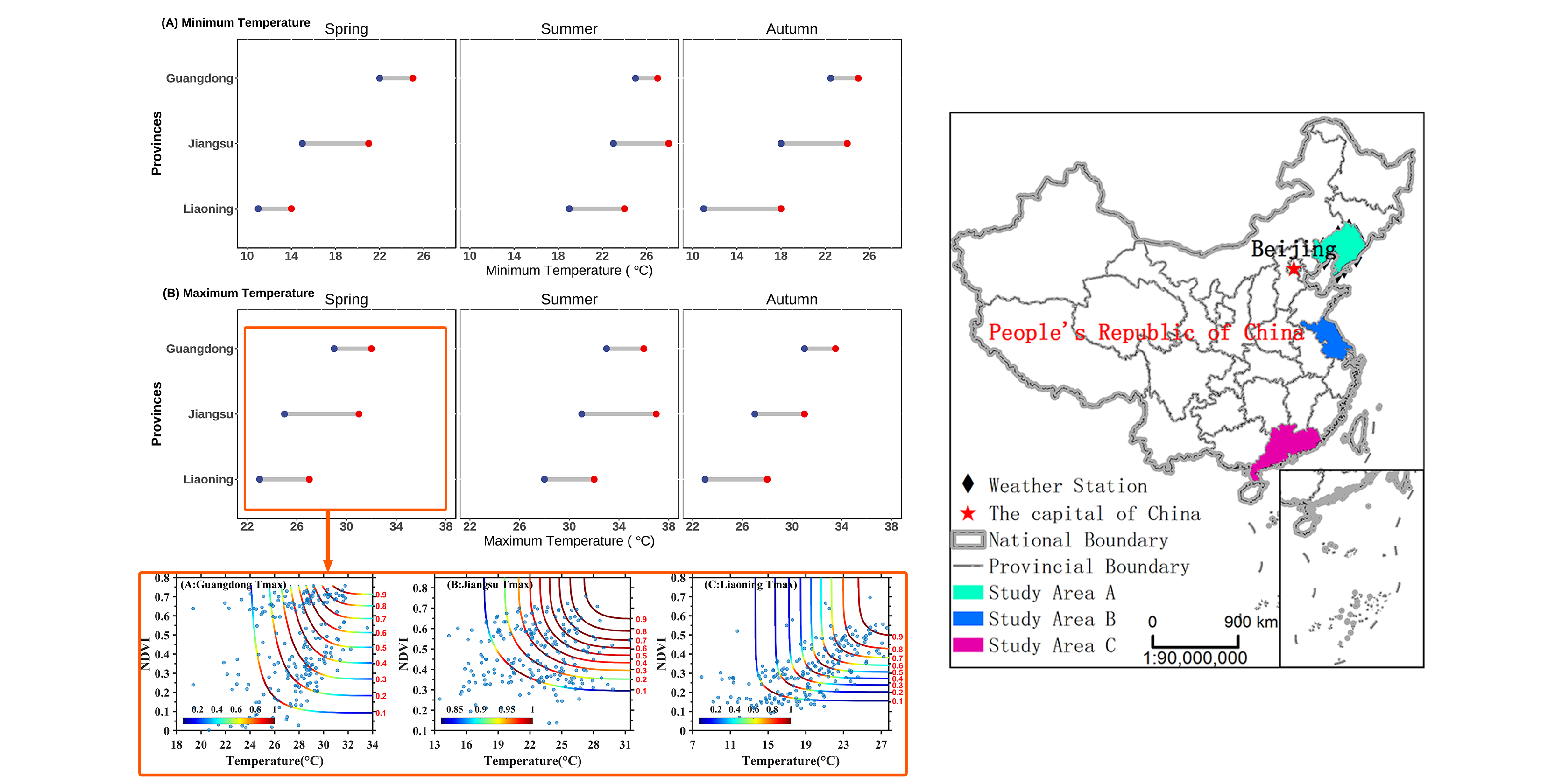
2.1. Research Areas

In this paper, Guangdong, Jiangsu and Liaoning are selected to represent typical climatic zones along the eastern coast of China (Figure 1). Guangdong is a southern province of China with a tropical and subtropical monsoon climate. Therefore, it has long summers and warm winters. The average annual temperature is from 20.4 to 23.1 °C. Jiangsu is an eastern-central province of China and is situated in a transitional area between temperate and subtropical zone. Generally, toward the south of the Huaihe River and sub-northern irrigation canal, humid subtropical climate zone is experienced, whereas, warm temperate climate zone is experienced toward the north. The annual average temperature is from 13 to 16 °C, increasing from northeast to southwest area. Liaoning is a northern coastal province in Northeast of China and is located in temperate monsoon climate zone. The temperature in this area is characterized by uneven spatial distributions, decreasing from the plain to the mountain area. The annual average temperature in Liaoning is from 7 °C to 11 °C.

2.2. Data and Preprocessing

2.2.1. Meteorological Data and Preprocessing

The daily temperature records from 1 January 1982 to 31 December 2016, were collected for the three provinces from 90 meteorological stations provided by the China Meteorological Administration (https://data.cma.cn/site/index.html). The stations were selected on the basis of the length of the time series, data completeness (missing values less than 5%) and spatial coverage. A series of quality control tests were applied to identify outliers at all stations and were marked with a quality control flag. The average daily temperatures were then extracted. It should be noted that the level of data completeness in the study exceeded the minimum requirement of 95%. At this level, scaling indices and scaling behaviors of the time series were not affected. The monthly regional maximum and minimum temperatures of Guangdong, Jiangsu and Liaoning provinces were calculated respectively according to the daily average air temperature.

According to the growth laws of vegetation in different climatic zones along the eastern coast of China, the months from April to May, June to August and September to October during the growing season are divided into spring, summer and autumn respectively, which approximately correspond to three physiological processes of the vegetation from turning green to maturing, from maturing to aging and from aging to hibernating [47]. Considering that the daily extreme maximum temperature occurs around 14:00 in most areas, and the daily extreme minimum temperature occurs before and after sunrise, Tmax and Tmin are taken as temperatures in daytime and at night, respectively.

2.2.2. NDVI Data and Preprocessing

NDVI data had a time span from 1982 to 2016, wherein Advanced Very High Resolution Radiometer (AVHRR) data and Moderate Resolution Imaging Spectroradiometer (MODIS) data were used, respectively. The AVHRR data came from National Aeronautics and Space Administration (NASA) Goddard Space Center (https://ltdr.modaps.eosdis.nasa.gov/cgi-bin/ltdr/ltdrPage.cgi) and had a time span from 1982 to 2010. This data was based on AVHRR observation data of NOAA07, NOAA09, NOAA11, NOAA16 and NOAA18.

The MODIS surface reflectance data came from the Terra satellite daily surface reflectance product MOD09GA developed by NASA’s MODIS terrestrial product group (https://ladsweb.modaps.eosdis.nasa.gov/). This product included daily surface reflectance data of MODIS in channels 1–7 with a spatial resolution of 500 m. This study used the surface reflectance data of MODIS in channels 1–7 in the growing season (from April to October) from 2010 to 2016. The data format was EOS-HDF and the projection mode was global sinusoidal projection (SIN).

For AVHRR data, a daily grid (the resolution is 0.05°) data set was generated after radiometric calibration, cloud detection and filtering, atmospheric correction, satellite drift correction and bidirectional reflectance distribution function (BRDF) processing. Surface reflectance data in bands 1–2 was processed into a Geo-TIFF format using IDL, the projection mode was set to Albers and the spatial resolution was defined as 5 km. For MOD09GA data, due to the difference in spatial resolutions of AVHRR NDVI data and MODIS NDVI data, in order to match with data temporally and spatially, the surface reflectance data of MODIS in bands 1–2 was processed into the Geo-TIFF format, the spatial resolution was resampled to 5 km and the Albers conical equal area projection was adopted. After quality inspection, image mosaic, subset extraction, cropping, format and projection conversion and other preprocessing processes, a MODIS NDVI data set was obtained. In this way, the time span of the AVHRR data set was extended to 1982–2016.

In order to eliminate the effects of cloud or noise in daily NDVI images as much as possible, daily NDVI data was generated first according to a NDVI calculation formula by using surface reflectance data of AVHRR and MODIS. Daily NDVIs of AVHRR and MODIS were then synthesized into monthly NDVI data, respectively, according to a daily quality control document through an MVC (Maximum Value Composites) method.

2.3. Methods

2.3.1. Maximum Value Composites

The maximum value composite (MVC) was proposed by Holben [53]. The specific formula of MVC [54] is as follows:

$$NDV{I}_i=Max\left(NDV{I}_{ij}\right),$$

(1)

where $NDV{I}_i$ refers to the NDVI in the ith month or the ith year; and $NDV{I}_{ij}$ refers to the NDVI data on the jth 15-day in the ith month or on the jth month in the ith year.

2.3.2. Copula Function Theory

The copula function raised by Sklar [55] can use the marginal distribution and correlation framework to build a multi-dimensional joint distribution copula function model [56]. The study selected eight copula function clusters [57,58,59,60], including: (1) BB1; (2) Clayton; (3) Frank; (4) Gaussian; (5) Gumbel; (6) Joe; (7) t; and (8) Tawn. These eight forms of the copula functions have always been common choices for related models due to their performances. The selected copula functions were used to establish a two-dimensional joint distribution of climate elements and NDVI.

Parameter Estimation

The parameters of the copula function were calculated by the non-parametric estimation method [61]. This technique is mainly related to the parameter θ of the copula. See

Table 1. Copula families and their closed-form mathematical description.

Copula Function Name	Mathematical Description
BB1 [62]	${\{1+{\left[{\left(u^{-{\theta }_1}-1\right)}^{{\theta }_2}+{\left(v^{-{\theta }_1}-1\right)}^{{\theta }_2}\right]}^{1/{\theta }_2}\}}^{-1/{\theta }_1}$
Clayton [57]	$max{\left(u^{-\theta }+v^{-\theta }-1,0\right)}^{-1/\theta }$
Frank [59]	$-\frac{1}{\theta }\ln \left[1+\frac{\left(\exp \left(-\theta u\right)-1\right)\left(\exp \left(-\theta v\right)-1\right)}{\exp \left(-\theta \right)-1}\right]$
Gaussian [59]	${{\displaystyle \int }}_{-\infty }^{{\varphi }^{-1}\left(u\right)}{{\displaystyle \int }}_{-\infty }^{{\varphi }^{-1}\left(v\right)}\frac{1}{2\pi \sqrt{1-{\theta }^2}}\exp \left(\frac{2\theta xy-x^2-y^2}{2\left(1-{\theta }^2\right)}\right)dxdy$
Gumbel [59]	$\exp \left\{-{\left[{\left(-\ln \left(u\right)\right)}^{\theta }+{\left(-\ln \left(v\right)\right)}^{\theta }\right]}^{1/\theta }\right\}$
Joe [59]	$1-{\left[{\left(1-u\right)}^{\theta }+{\left(1-v\right)}^{\theta }-{\left(1-u\right)}^{\theta }{\left(1-v\right)}^{\theta }\right]}^{1/\theta }$
t [59]	${{\displaystyle \int }}_{-\infty }^{t_{{\theta }_2}^{-1}\left(u\right)}{{\displaystyle \int }}_{-\infty }^{t_{{\theta }_2}^{-1}\left(v\right)}\frac{\mathsf{\Gamma }\left(\left({\theta }_2+2\right)/2\right)}{\mathsf{\Gamma }\left({\theta }_2/2\right)\pi {\theta }_2\sqrt{1-{\theta }_1^2}}{\left(1+\frac{x^2-2{\theta }_{1}xy+y^2}{{\theta }_2}\right)}^{\left({\theta }_2+2\right)/2}dxdy$
Tawn [63]	$\exp \left\{\ln \left(u^{\left(1-{\theta }_1\right)}\right)+\ln \left(v^{\left(1-{\theta }_2\right)}\right)-{\left[{\left(-{\theta }_1\ln \left(u\right)\right)}^{{\theta }_3}+{\left(-{\theta }_2\ln \left(v\right)\right)}^{{\theta }_3}\right]}^{1/{\theta }_3}\right\}$

for various copula function forms:

Equation (2) shows the relationship between θ and τ (Kendall correlation coefficient). By calculating τ from the measured data, the corresponding joint distribution parameters can be obtained.

$$\tau =1- \frac{1}{\theta },$$

(2)

Verification and Evaluation

To quantitatively evaluate the fitting error and select the appropriate copula function, Akaike information criterion (AIC), Bayesian information criterion (BIC) [64] and root mean square error (RMSE) [65] were employed as the criteria for selecting the copula function clusters.

$$AIC= -2\iota \left(\widehat{\theta }|y\right)+2K,$$

(3)

$$BIC= -2\iota \left(\widehat{\theta }|y\right)+Kln\left(n\right),$$

(4)

K was the number of estimated parameters in the model including the intercept and $\iota (\widehat{\theta }|y)$ was a log-likelihood at its maximum point of the estimated model; n was a sample size. The rule of selection was that the smaller the value of AIC was, the better the model was, and so did the BIC.

$$RMSE= \sqrt{\frac{1}{n}{{\displaystyle \sum }}_{i=1}^n{\left(X_C\left(i\right)-X_O\left(I\right)\right)}^2} ,$$

(5)

where n is the number of observations; Xc is the theoretical probability of copula and Xo is the empirical probabilities of observations.

Correlation Analysis and Establishment of Marginal Distribution Function

In order to determine whether there was a correlation between the NDVI and monthly mean temperature and monthly precipitation, this paper established a joint distribution function and adopted Kendall, Pearson and Spearman rank correlation coefficients to analyze the correlation between the climate elements and the NDVI.

Multivariate Copula Analysis Toolbox (MvCAT), as a general software toolbox, uses Markov chain Monte Carlo simulations (MCMC) to estimate copula parameters [66]. It was adopted to study the dependency structure between variables and select the optimal marginal distribution function for each variable. Distribution functions include: (1) Beta; (2) Birnbaum–Saunders; (3) exponential; (4) extreme value; (5) gamma; (6) generalized extreme value; (7) generalized Pareto; (8) inverse Gaussian; (9) logistic; (10) log-logistic; (11) log-normal; (12) Nakagami; (13) normal; (14) Rayleigh; (15) Rician; (16) T location scale; and (17) Weibull distributions. The parameters are estimated by the maximum likelihood approach. Detailed descriptions about these distributions refer to Sadegh et al. [67].

Joint Probability Distribution

For the sake of the study of the joint probability of Tmax–NDVI and Tmin–NDVI, the marginal distributions of Tmax, Tmin and NDVI were calculated, respectively, and the parameters of this function were obtained. The comparison between a fitting result of the function and the actual data was evaluated using a quantile–quantile plot. Based on the univariate marginal function, a two-dimensional copula function was constructed, and three goodness-of-fit evaluation indexes of AIC, BIC and RMSE were used to select the optimal copula function type from the copula function clusters [68].

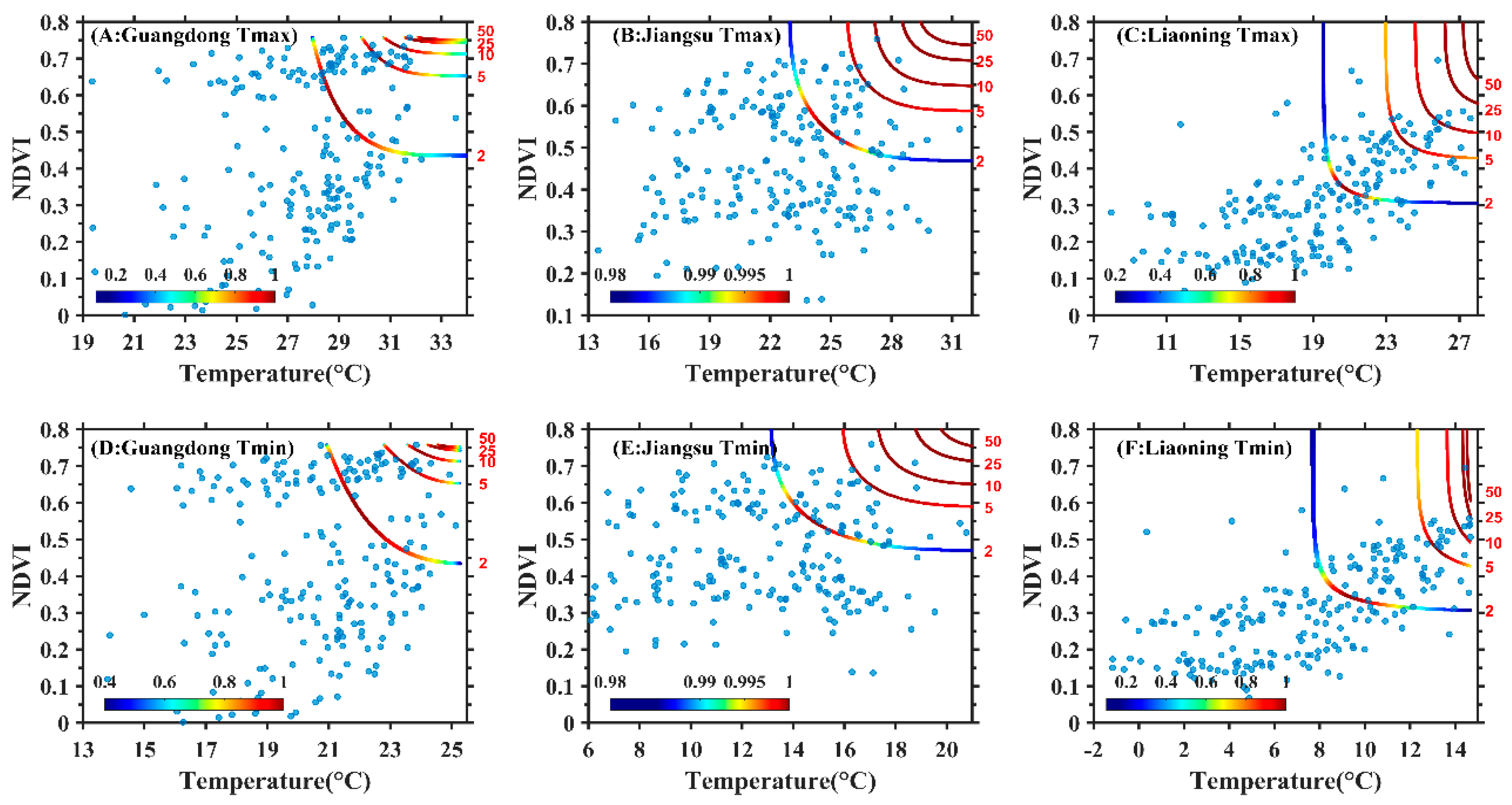
The Return Period of NDVI and Tmax/Tmin

The return period refers to the time when the value of the random variable appears in a longer period [69]. Calculating the return periods of the NDVI under different maximum and minimum temperature conditions can provide valuable information for a more meticulous study of daytime and nighttime warming asymmetry affect the NDVI. This paper calculates a bivariate joint return period because the univariate recurrence interval or return period often leads to overestimation or underestimation of the risk rate of an event [70]. It is defined that in the joint return period, $X\ge x$ and $Y\ge y$.

$$T_{joint}=\frac{E\left(L\right)}{P(X\ge x,Y\ge y)}=\frac{E\left(L\right)}{1-F_X\left(x\right)-F_Y\left(y\right)+C\left(F_X\left(x\right),F_Y\left(y\right)\right)},$$

(6)

In the above formulas, Tjoint represented the joint return period for $X\ge x$ and $Y\ge y$; and E(L) showed an expected value of the time interval at which continuous events start. Detailed discussions on the relationships between univariate and bivariate return periods could be found in Shiau [70].

3. Results

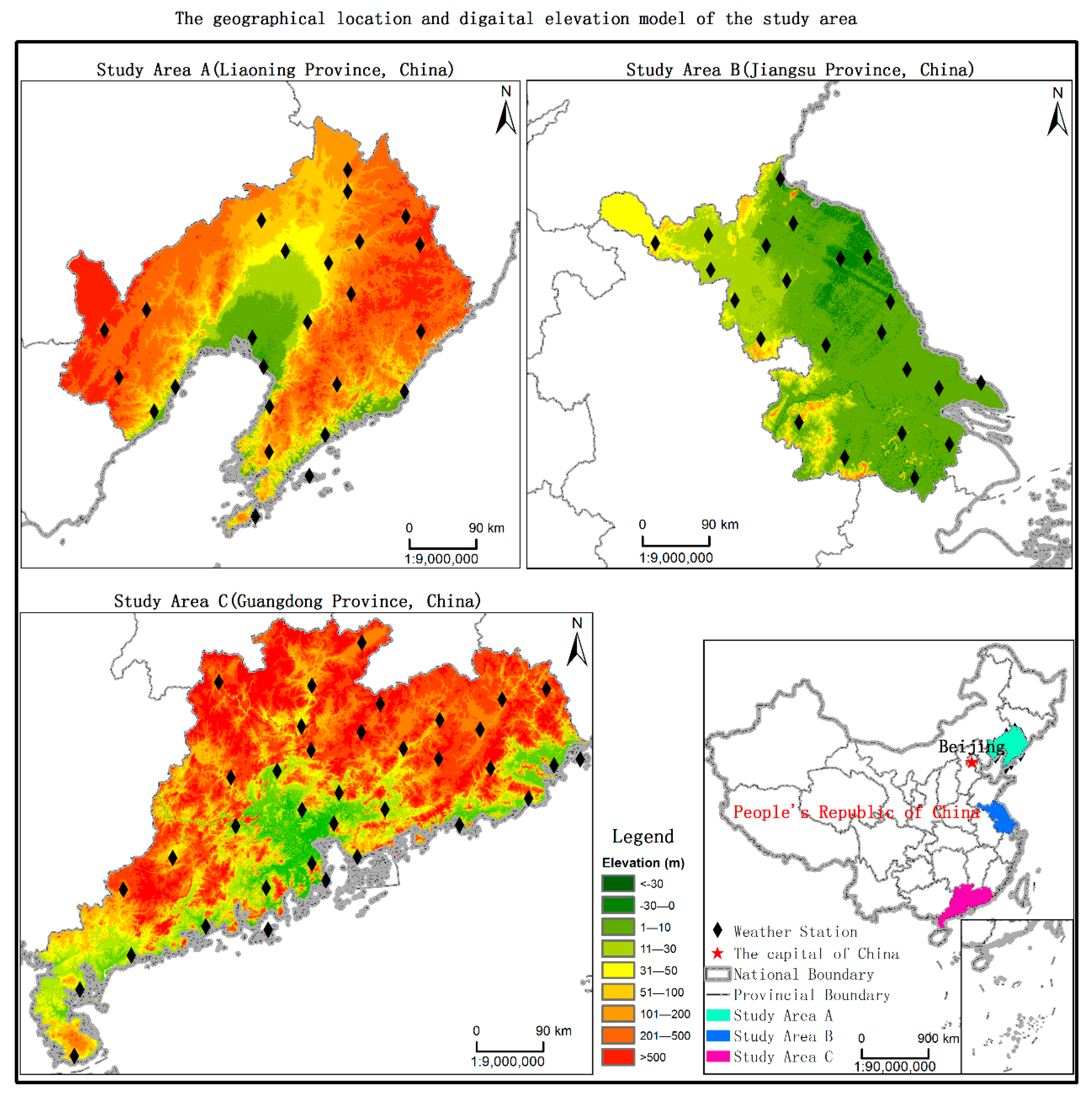
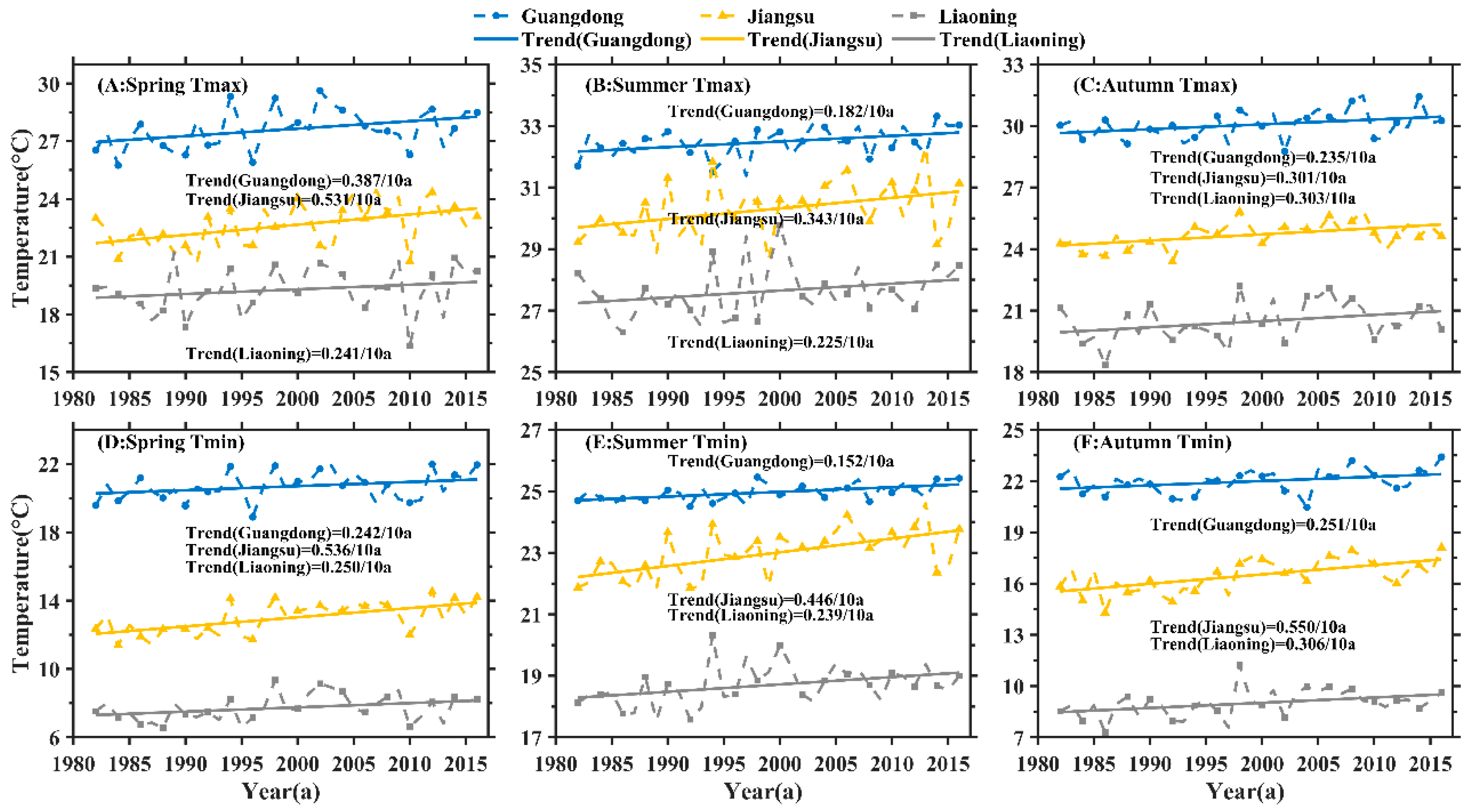
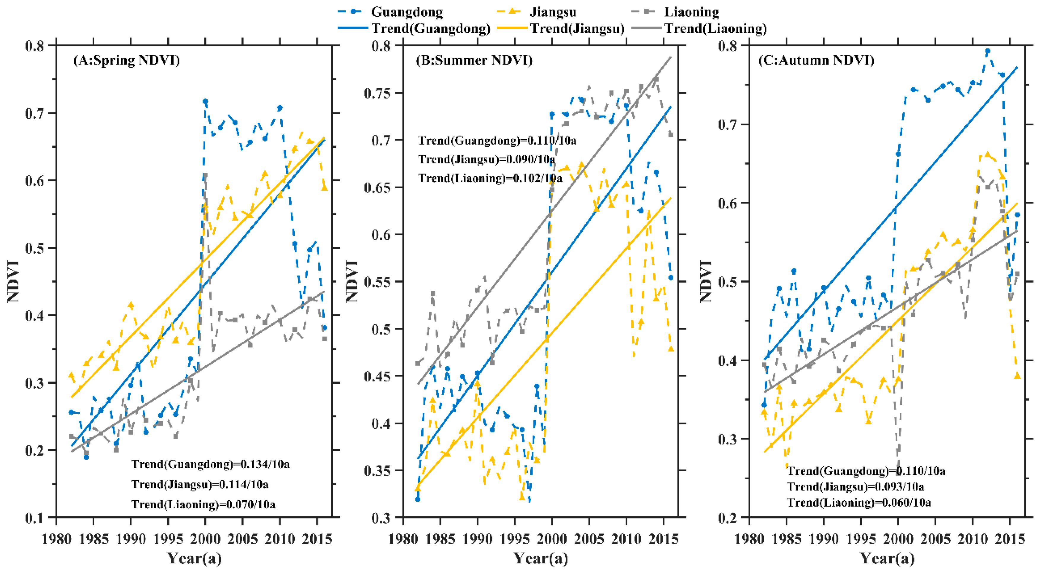
3.1. Trend Analysis of Seasonal Daytime and Nighttime Temperature Increases and NDVI

From Guangdong to Liaoning, it spanned tropical, subtropical and temperate zones, and climate and NDVI change rates in different regions varied markedly. Figure 2 showed a change trend of the maximum temperatures (Tmax) and the minimum temperatures (Tmin) in Guangdong, Jiangsu and Liaoning in spring, summer and autumn.

An obvious rising trend in Tmax was shown in Guangdong, Jiangsu and Liaoning. In spring, the rising rates per 10a from large to small were Jiangsu, Guangdong and Liaoning. The rising rates per 10a in summer were Jiangsu > Liaoning > Guangdong. However, in autumn, the rising rates per 10a from large to small were Liaoning, Jiangsu and Guangdong. A significant increase trend in Tmin was shown in the three regions in each season. The increase rates of Tmin per 10a in different seasons were the fastest in Jiangsu, followed by Liaoning and the slowest in Guangdong. At the same time, the rates of daytime and nighttime temperature increases in the three regions also showed significant differences. In Guangdong, the ratios of Tmax and Tmin warming rates in spring, summer and autumn were 1.6, 1.2 and 0.94 respectively. In Jiangsu, the ratios of daytime and nighttime warming rates in different seasons were 0.99, 0.77 and 0.55 respectively. In Liaoning, the ratios of daytime and nighttime warming rates were 0.96, 0.94 and 0.99 in its respective season.

The daytime and nighttime temperature increases in the three regions showed asymmetric changes in different seasons, with obvious seasonal differences. In spring and summer, the warming rates in the daytime in Guangdong were faster than those at night, and the warming rate at nighttime in autumn was faster than that in the daytime. However, the warming rates in the daytime in the three seasons in Jiangsu and Liaoning were slower than those at nighttime.

Figure 3 showed the changing trends of NDVI in spring, summer and autumn in the three regions. The NDVIs of the three regions all showed an obvious increase trend, with a sharp jump phenomenon in NDVI around 2000. The increase rates of NDVI in spring were Guangdong > Jiangsu > Liaoning. In summer, the increase rates of NDVI from large to small were Guangdong, Liaoning and Jiangsu. In autumn, the increase rates of NDVI from large to small were Guangdong, Jiangsu and Liaoning. For different seasons of the same region: in Guangdong province, the increase rates of NDVI were spring > summer = autumn; In Jiangsu province, the increase rates of NDVI from large to small were spring, autumn and summer; In Liaoning province, the increase rates of NDVI from large to small were summer, spring and autumn.

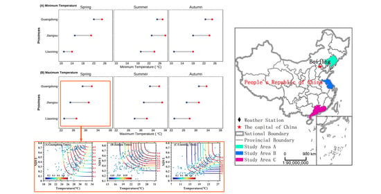
3.2. Construction of Copula Function Cluster of the Maximum Temperature, Minimum Temperature and NDVI

Laws of asymmetry and seasonal differences in daytime and nighttime temperature increases in different latitudes led to temporal and spatial differences in the response of vegetation to temperature increase. Correlation analysis of Tmax, Tmin and NDVI in spring, summer and autumn in Guangdong, Jiangsu and Liaoning were performed, respectively. Kendall, Pearson and Spearman correlation coefficients were used to measure the correlation of two-dimensional variables. The calculation results were shown in

Table 2. Correlation coefficients of Tmax–NDVI in spring, summer and autumn in Guangdong, Jiangsu and Liaoning.

Province	Season	Kendall	p Value	Spearman	p Value	Pearson	p Value
Guangdong	spring	0.284	0.000	0.401	0.000	0.374	0.000
Jiangsu	spring	0.056	0.227	0.083	0.230	0.116	0.095
Liaoning	spring	0.468	0.000	0.660	0.000	0.619	0.000
Guangdong	summer	0.224	0.000	0.327	0.000	0.331	0.000
Jiangsu	summer	0.366	0.000	0.522	0.000	0.532	0.000
Liaoning	summer	0.250	0.000	0.370	0.000	0.365	0.000
Guangdong	autumn	0.150	0.001	0.219	0.001	0.228	0.001
Jiangsu	autumn	0.418	0.000	0.591	0.000	0.585	0.000
Liaoning	autumn	0.598	0.000	0.789	0.000	0.771	0.000

and

Table 3. Correlation coefficients of Tmin–NDVI in spring, summer and autumn in Guangdong, Jiangsu and Liaoning.

Province	Season	Kendall	p Value	Spearman	p Value	Pearson	p Value
Guangdong	spring	0.177	0.000	0.258	0.000	0.234	0.001
Jiangsu	spring	0.039	0.402	0.062	0.372	0.086	0.213
Liaoning	spring	0.501	0.000	0.696	0.000	0.662	0.000
Guangdong	summer	0.148	0.000	0.219	0.000	0.212	0.000
Jiangsu	summer	0.397	0.000	0.572	0.000	0.585	0.000
Liaoning	summer	0.233	0.000	0.335	0.000	0.359	0.000
Guangdong	autumn	0.090	0.052	0.128	0.064	0.087	0.209
Jiangsu	autumn	0.409	0.000	0.581	0.000	0.568	0.000
Liaoning	autumn	0.595	0.000	0.787	0.000	0.771	0.000

.

The correlation of the maximum temperature and NDVI and the minimum temperature and NDVI in spring in Jiangsu, and the correlation of the minimum temperature and NDVI in autumn in Guangdong failed to pass a significance test. The correlations of temperatures in daytime and at night and NDVI in other cases showed a significant positive correlation. However, the correlations of Tmax and NDVI, and Tmin and NDVI in the three regions in different seasons were significantly different. Moreover, the correlations of Tmax and NDVI, and Tmin and NDVI in different seasons in the same area also showed significant differences. In summary, it could be seen that the asymmetry of daytime and nighttime temperature increases had a very obvious impact on NDVI of the typical coastal climate zone in China, and had regional and temporal differences.

According to the optimal AIC, BIC and RMSE in

Table 4. Copula function cluster selection criteria for Tmax–NDVI in Guangdong, Jiangsu and Liaoning.

	PROVINCE	Guangdong	Jiangsu	Liaoning
	Copula Function	BB1	BB1	Frank
Spring	AIC	−177.71	−193.27	−190.29
Spring	BIC	−177.04	−192.60	−189.96
Spring	RMSE	0.21	0.14	0.16
Summer	AIC	−277.29	−315.40	−271.40
Summer	BIC	−276.54	−314.65	−271.03
Summer	RMSE	0.22	0.12	0.24
Autumn	AIC	−193.76	−198.09	−204.55
Autumn	BIC	−193.09	−197.43	−204.22
Autumn	RMSE	0.14	0.13	0.11

and

Table 5. Copula function cluster selection criteria for Tmin–NDVI in Guangdong, Jiangsu and Liaoning.

	PROVINCE	Guangdong	Jiangsu	Liaoning
	Copula Function	BB1	BB1	Frank
Spring	AIC	−177.71	−193.27	−190.29
Spring	BIC	−177.04	−192.60	−189.96
Spring	RMSE	0.21	0.14	0.16
Summer	AIC	−277.29	−315.40	−271.40
Summer	BIC	−276.54	−314.65	−271.03
Summer	RMSE	0.22	0.12	0.24
Autumn	AIC	−193.76	−198.09	−204.55
Autumn	BIC	−193.09	−197.43	−204.22
Autumn	RMSE	0.14	0.13	0.11

, the optimal Tmax–NDVI copula functions of Guangdong, Jiangsu and Liaoning were BB1, BB1 and Frank, respectively, and their corresponding evaluation index values were all smaller than it of the other eight copula functions. Similarly, the Tmin–NDVI optimal copula functions of the three provinces were BB1, Clayton and Frank, respectively. These copula functions had an optimal fitting effect and were more suitable for describing the joint distribution characteristics of Tmax–NDVI and Tmin–NDVI. Therefore, BB1, BB1 and Frank functions and BB1, Clayton and Frank copula functions were used in this paper respectively to establish a two-dimensional joint probability distribution model of Tmax–NDVI and Tmin–NDVI in the three regions.

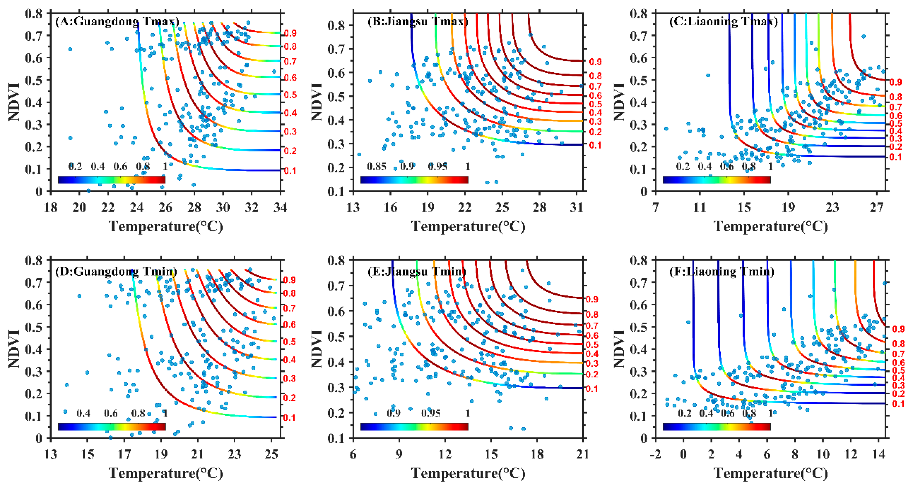
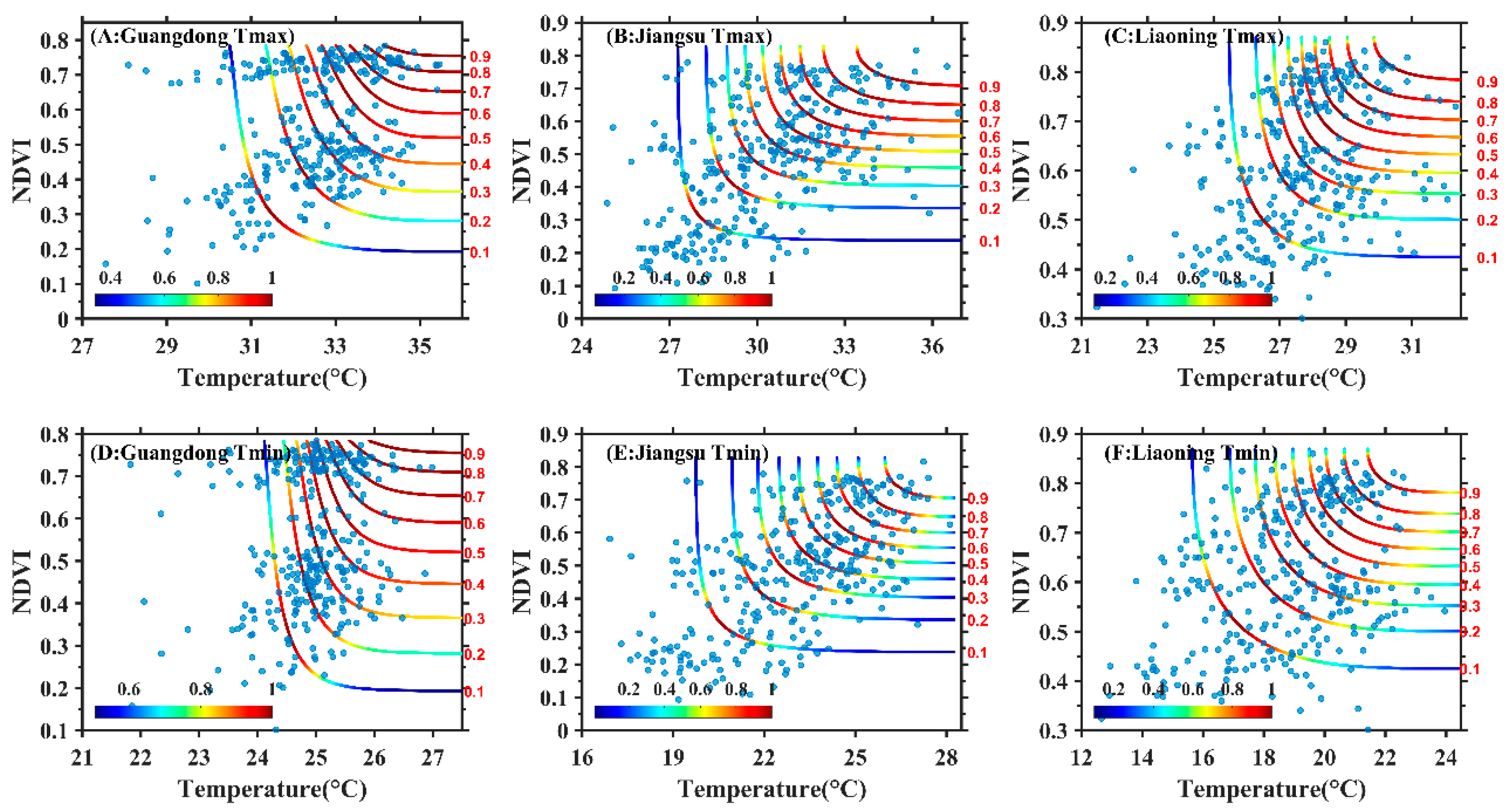
3.3. Joint Probability Distribution Characteristics of Maximum Temperature, Minimum Temperature and NDVI

According to the optimal copula function, the joint probability distributions and return periods of Tmax–NDVI and Tmin–NDVI in spring, summer and autumn during the growing seasons in Guangdong, Jiangsu and Liaoning were calculated respectively.

Figure 4 showed a joint probability distribution relationship of the monthly average maximum temperature and NDVI (Figure 4A–C) and a joint probability distribution relationship of the monthly average minimum temperature and NDVI (Figure 4D–F) in spring of Guangdong, Jiangsu and Liaoning. The joint probability distribution function could clearly reflect the correlations of Tmax and NDVI, and Tmin and NDVI in different value ranges. The most significant feature in the figure was an asymmetric and tilted dependency structure of monthly scale data. It had a small impact on NDVI when a minimum value was taken from Tmax and Tmin, and had a significant impact on NDVI when a maximum value was taken from Tmax and Tmin. The interval distribution of Tmax–NDVI and Tmin–NDVI when the joint probabilities were 0.1–0.9, respectively, can be derived according to a contour map. When Tmax and Tmin were fixed values, NDVI was larger; or when NDVI was fixed, Tmax and Tmin were larger, and their joint probabilities were higher. The joint probabilities of different combinations of Tmax, Tmin and NDVI on the same contour line also showed significant differences. For example, in Figure 4A, when Tmax was greater than 29 °C in Guangdong, the joint probability was greater than 0.7, and the plant growth was more likely to be in a good state. However, on the same probability contour line (probability = 0.7), the probability when Tmax was in an interval of 29–32 °C was greater than that in an interval of 32–34 °C. Obviously, when Tmax was too high, the probability of plant growth in a good state decreased, resulting in a phenomenon of inhibiting plant growth.

In spring, when Tmax(s) in Guangdong, Jiangsu and Liaoning were in the intervals of 29–32 °C, 25–31 °C and 23–27 °C, or when Tmin(s) were in the intervals of 22–25 °C, 15–21 °C and 11–14 °C, there was a high probability (greater than 0.7) that NDVI is relatively high (greater than 0.6), which indicated that the plant growth in the three regions was likely to be in a good state.

Figure 5 showed two-dimensional contour lines of joint return periods of Tmax–NDVI and Tmin–NDVI in Guangdong, Jiangsu and Liaoning. The corresponding return periods when Tmax, Tmin or NDVI was greater than or equal to a specific value could be calculated according to the contour map. It reflected the combinations of Tmax, Tmin or NDVI greater than or equal to the specific values when the return periods were 2 years, 5 years, 10 years, 25 years and 50 years. The shorter the joint return period, the larger the value ranges of Tmax, Tmin and NDVI, which meant that the possibility of a shorter return period for NDVI was higher when Tmax and Tmin were fixed. In spring, Tmax(s) in Guangdong, Jiangsu and Liaoning were in larger intervals (28–33 °C, 22.5–33.5 °C and 17–22 °C respectively), or Tmin(s) were in larger intervals (21–25 °C, 14.5–21 °C and 13–14.5 °C), resulting in a maximum probability of the shorter return period for NDVI in this case. The NDVI was greater than 0.3 in the above temperature ranges, which indicated that plant growth in good condition occurred most frequently. When the values of Tmax, Tmin and NDVI were large enough, their return periods may even exceed 50 years, which indicated that the phenomenon of inhibiting plant growth appeared when the temperature exceeded a certain threshold. The higher the temperature, the greater the inhibition for plant growth is.

Figure 6 showed the joint probability distributions between the monthly average maximum temperature and NDVI and between the monthly average minimum temperature and NDVI in summer in Guangdong, Jiangsu and Liaoning from 1982 to 2016. It could be seen from Figure 6 that it had a smaller impact on NDVI when a minimum value was taken from Tmax and Tmin, and had a significant impact on NDVI when a maximum value was taken from Tmax and Tmin. In summer, when Tmax(s) in Guangdong, Jiangsu and Liaoning were in the intervals of 33–36 °C, 31–37 °C and 28–32 °C, or when Tmin(s) were in the intervals of 25.5–27.5 °C, 24–27 °C and 20–24 °C, there was a high probability (greater than 0.7) that NDVI was relatively high (greater than 0.6), which indicated that the plant growth in the three regions was likely to be in a good state.

Figure 7 showed two-dimensional contour lines of the joint return periods of Tmax and NDVI, and Tmin and NDVI in summer in Guangdong, Jiangsu and Liaoning. It reflected the combinations of Tmax, Tmin or NDVI greater than or equal to specific values when the return periods were 2 years, 5 years, 10 years, 25 years and 50 years. The shorter the joint return period, the larger the value ranges of Tmax, Tmin and NDVI, which meant that NDVI had a greater possibility of having a shorter return period when Tmax and Tmin were fixed. In summer, Tmax(s) in Guangdong, Jiangsu and Liaoning were in larger intervals of 33–36 °C, 30–36.5 °C and 27.5–33 °C, or Tmin(s) were in larger intervals of 25–27 °C, 23–28 °C and 19–24 °C, and NDVI had the greatest probability of having a smaller return period. NDVIs were greater than 0.5 in the above temperature ranges, which indicated that plant growth in good condition occurred most frequently.

Figure 8 showed joint probability distribution relationships between the monthly average Tmax and NDVI, and between the monthly average Tmin and NDVI in autumn in Guangdong, Jiangsu and Liaoning from 1982 to 2016, which can clearly reflect the correlations between Tmax and NDVI and between Tmin and NDVI in different value ranges. It can be seen from Figure 8 that it had a smaller impact on NDVI when a minimum value was taken from Tmax and Tmin, and had a significant impact on NDVI when a maximum value was taken from Tmax and Tmin. In autumn, when Tmax(s) in Guangdong, Jiangsu and Liaoning were in the intervals of 31–33.5 °C, 27–31 °C and 23–28 °C, or when Tmin(s) were in the intervals of 22.5–25 °C, 18–24 °C and 11–18 °C, there was a high probability (greater than 0.7) that NDVI was relatively high (greater than 0.6), which indicated that the plant growth in the three regions was likely to be in a good state.

Figure 9 showed two-dimensional contour lines of the joint return periods of Tmax, Tmin and NDVI in autumn in Guangdong, Jiangsu and Liaoning, which reflected the combinations of Tmax, Tmin or NDVI greater than or equal to specific values when the return periods were 2 years, 5 years, 10 years, 25 years and 50 years. The shorter the joint return period, the larger the value ranges of Tmax, Tmin and NDVI, which meant that NDVI had a greater possibility of having a shorter return period when Tmax and Tmin were fixed. In autumn, Tmax(s) in Guangdong, Jiangsu and Liaoning were in larger intervals of 30–34 °C, 25–31.5 °C and 21–28 °C, or Tmin(s) were in larger intervals of 22–25.5 °C, 17–25 °C and 9–18.5 °C, resulting in a highest probability of a shorter return period for NDVI in this case. NDVIs were greater than 0.5 in the above temperature ranges, which indicated that plant growth in good condition occurred most frequently.

4. Discussion

The typical temperature zones along the eastern coast of China presented the asymmetry of daytime and nighttime warming in different seasons, showing a significant rising trend, and the geographical distribution of the temperature increase trend was obviously different in respective seasons. This conclusion was basically consistent with the seasonal evolution characteristics of daytime and nighttime warming in part of regions in China. Secondly, there were obvious asymmetric change characteristics of daytime and nighttime warming on a seasonal scale [46,71]. The research results from Xu et al. [72] showed that in the high latitudes of the Northern Hemisphere, the rate of temperature increase in summer was faster than that in spring and autumn, and the seasonal temperature difference showed a reduction trend. Asymmetric seasonal temperature increases in daytime and at night undoubtedly increased the complexity of vegetation in response to seasonal temperature changes.

4.1. Effects of the Asymmetry of Daytime and Nighttime Temperature Increases on Vegetation Activities

The photosynthesis of most plants takes place in daytime, while the respiration occurs throughout the day. Therefore, the uneven warming rates in daytime and at night affected the dynamic changes of vegetation by acting on the physiological process of vegetation [73,74,75]. Peng et al. [15] analyzed the inter-annual correlation variations between NDVI and Tmax and between NDVI and Tmin in the Northern Hemisphere, and found that the increase in Tmax in the northern region often had a positive effect on the increase in NDVI, and Tmin and NDVI often showed a negative correlation. Tan et al. [47] found that the daytime warming in summer in the Northern Hemisphere was not conducive to the growth of vegetation in arid regions in temperate zones, but the daytime warming in spring could be conducive to the increase in NDVI of vegetation in cold regions. This study found that the warming rates in the daytime in spring and summer in Guangdong were faster than that at night; meanwhile, the maximum temperature in the daytime had a greater impact on plant growth than the minimum temperature at night. The warming rates in the daytime in summer and autumn in Jiangsu were lower than that at night, while the maximum temperature in summer had less impact on plant growth than the minimum temperature, and the opposite is true in autumn. This might be due to the high Tmax in summer in Jiangsu. When the continuous increase in Tmax exceeded an optimum temperature range for plants, guard cells of vegetation leaves were closed, the photosynthesis rate was slowed, the synthesis rate of organic matters was reduced and the net accumulation of organic matters was reduced, resulting in an adverse effect on its growth and development. The daytime warming in spring in Liaoning had a weaker effect on plant growth than that at night, and the opposite is true in summer and autumn. This was because the nighttime warming in spring can increase the autotrophic respiration rate of vegetation, reduce the volume of endosperm cells in the mature stage of plants, shorten the filling period of plants and have a negative impact on the increase in NDVI [76,77,78]. It was worth noting that the increase in autotrophic respiration at night may also stimulate the increase in photosynthesis ability of vegetation in the next day by virtue of a compensation action. In addition, the temperature increase at night could reduce the occurrence frequency of frost disasters [79,80] and regulate the carbohydrate content in plant leaves [81], which had a positive effect on the increase in vegetation productivity. In summer and autumn, the warming rates in the daytime were slower than that at night. This was probably because Tmax was in a suitable temperature interval. The increase in Tmax might promote the increase in vegetation NDVI by improving the availability of soil nitrogen, the activity of photosynthetic enzymes and extending the growth cycle of vegetation.

4.2. Effects of Non-Uniform Temperature Increase in Different Seasons on Vegetation Activities

The correlation between the dynamic changes of NDVI and temperatures in the daytime and at night showed significant differences as a result of the difference in seasons and latitude intervals. In spring, the temperatures in daytime and at night were positively correlated with NDVIs in Guangdong (low latitude) and Liaoning (high latitude). This might be related to the advancement of the growing season caused by global warming [82], or might also be due to the fact that the temperature increase in daytime played a positive role in the advancement of the leaf extension stage and returning green stage of vegetation [39]. Compared with Guangdong, Liaoning had a higher degree of correlation between the daytime and nighttime warming and NDVI. This was because Liaoning was located at high latitudes and had poor thermal conditions, so the daytime and nighttime warming had a greater effect on vegetation growth. The effects of temperature increase at night on vegetation growth in Guangdong were spring>summer>autumn; and the effects of temperature increase in daytime on vegetation growth were manifested to be spring<summer. The effect of temperature increase in daytime on vegetation growth in Jiangsu was greater in summer than in autumn, and the opposite law was observed at night. The effects of daytime and nighttime temperature increases on vegetation growth in Liaoning were autumn>spring>summer. This might be due to the fact that the number of hours of sunshine and solar radiation in autumn were lower than those in spring, and the productivity of each day of extension of the vegetation growth cycle was lower in autumn than in spring [83]. On the other hand, the duration of photosynthesis and vegetation productivity in autumn were more sensitive to temperature than that in spring [84]. In high latitudes, the daytime and nighttime warming in summer had the least effect on vegetation growth. Because Tmax in summer was close to the optimum temperature for vegetation growth in most area, the sensitivity of NDVI to Tmax was relatively low.

There were obvious seasonal differences in the asymmetric change characteristics of daytime and nighttime warming in these three regions. The warming rates in the daytime in Guangdong in spring and summer were faster than that at night, and the warming rate at nighttime in autumn was faster than that in the daytime. However, the warming rates in the daytime in Jiangsu and Liaoning were slower than that at night. In spring, the daytime warming had a greater impact on plant growth than the nighttime warming in Guangdong, while Liaoning had the opposite trend. In summer, the daytime warming was stronger than the nighttime warming in Guangdong and Liaoning, while the daytime warming was weaker than the nighttime warming in Jiangsu. In autumn, the daytime warming was stronger than the nighttime warming in Liaoning and Jiangsu. It could be seen that regions of different latitudes showed the asymmetry of daytime and nighttime temperature increases in respective seasons, and the response of plant growth in different regions on the asymmetry of seasonal daytime and nighttime temperature increases also showed a significant difference.

4.3. Exploration of Dynamic Changes of Temperature and NDVI Using Copula Function

According to Table 2 and Table 3, the correlation between daytime and nighttime temperature increases in spring in Jiangsu and NDVI and the correlation between the temperature increase at night in autumn in Guangdong and NDVI failed to pass a significance test. Correlation coefficients were widely used as a method to study the correlation between variables, but could not be intended to distinguish the dynamic correlations of the variables in different intervals, and thus failed to rule out the possibility of “false correlation” between variables. These problems can be solved very well by using the copula function theory. Using the copula function, more detailed and real dynamic change laws of temperatures and NDVI can be found. The daytime and nighttime temperature increases in spring in Jiangsu and the temperature increase at night in autumn in Liaoning were weak, and thus had less of an impact on plant growth. However, when the temperature increases were located in a suitable temperature range, they were strongly dependent on NDVI and had a greater impact on plant growth. In Guangdong, Jiangsu and Liaoning, when Tmax or Tmin was in a suitable temperature range, there was a greatest probability that NDVI had a smaller return period, which indicated that the plant growth in good condition occurred most frequently. However, when the values of Tmax, Tmin and NDVI were large enough, their return periods may even exceed 50 years, which indicated that the phenomenon of inhibiting plant growth appeared when the temperature exceeded a certain threshold. The higher the temperature, the greater the inhibition of plant growth is, and the lower the probability of good condition.

Owing to the issues of a relatively low resolution of remote sensing data and the heterogeneity of vegetation types within the same area, it was still difficult to obtain ideal results. Therefore, in future researches, it was necessary to introduce vegetation classification data of higher resolution into the study of the dynamic effects of daytime and nighttime temperature increases on global vegetation. Therefore, different climate change response policies were proposed for different vegetation types, and appropriate vegetation protection measures was established in accordance with local conditions, which would be more conducive to maintaining the balance of the natural ecosystem.

5. Conclusions

In this paper, meteorological and satellite remote sensing data sets from 1982 to 2016 in a typical temperature zone along the eastern coast of China were used to analyze the effects of asymmetric changes in daytime and nighttime warming in different seasons during the growing season on NDVI. The main conclusions were summarized as follows.

(1) In the past 35 years, the trends of seasonal daytime and nighttime temperature increases in the three regions were significant, resulting in asymmetric characteristics of rates of daytime and nighttime temperature increases. The rate of temperature increase in daytime in spring and summer in Guangdong was faster than that at night, and the opposite pattern was observed in autumn. The rates of temperature increases in spring, summer and autumn in Jiangsu and Liaoning were slower than that at night. The rates of daytime and nighttime warming vary significantly at different latitudes, showing an increase from low latitude (Guangdong) to middle latitude (Jiangsu), and a decrease from middle latitude (Jiangsu) to high latitude (Liaoning).

(2) The effects of daytime and nighttime temperature increases on vegetation in the three regions showed obvious seasonal differences. The effects of temperature increase at night on vegetation growth in Guangdong were spring > summer; and the effects of temperature increase in daytime on vegetation growth were manifested as spring > summer > autumn. In Jiangsu, the effects of daytime and nighttime temperature increases in summer on vegetation growth were less than that in autumn. The effects of daytime and nighttime temperature increases in summer on vegetation growth were manifested as autumn > spring > summer in Liaoning.

(3) The joint probability distribution functions of Tmax and NDVI, and Tmin and NDVI in Guangdong, Jiangsu and Liaoning were presented below: when Tmax and Tmin were fixed and NDVI was larger, or when NDVI was fixed and Tmax and Tmin were larger, the joint probability was larger, which indicated that it had less impact on NDVI when a minimum value was taken from Tmax and Tmin, and had a significant impact on NVDI when a maximum value was taken from Tmax and Tmin.

(4) The shorter the return period, the larger the value ranges of a climate factor and NDVI, which meant that NDVI had a higher possibility of having a shorter return period when the climate factor was fixed. The larger the climate factor, the longer the return period, which indicated that a phenomenon of inhibiting plant growth was more likely to occur when the climate factor exceeded a certain threshold.

References

1. Gong, Z.; Zhao, S.; Gu, J. Correlation analysis between vegetation coverage and climate drought conditions in North China during 2001–2013. J. Geogr. Sci. 2017, 27, 143–160. [Google Scholar] [CrossRef]
2. Zhang, W.; Döscher, R.; Koenigk, T.; Miller, P.A.; Jansson, C.; Samuelsson, P.; Wu, M.; Smith, B. The Interplay of Recent Vegetation and Sea Ice Dynamics—Results from a Regional Earth System Model Over the Arctic. Geophys. Res. Lett. 2020, 47, e2019GL085982. [Google Scholar] [CrossRef]
3. Teixeira, A.H.D.C.; Bastiaanssen, W.G.M.; Ahmad, M.D.; Moura, M.S.B.; Bos, M.G. Analysis of energy fluxes and vegetation-atmosphere parameters in irrigated and natural ecosystems of semi-arid Brazil. J. Hydrol. 2008, 362, 110–127. [Google Scholar] [CrossRef] [Green Version]
4. Balzarolo, M.; Vicca, S.; Nguy-Robertson, A.L.; Bonal, D.; Elbers, J.A.; Fu, Y.H.; Grünwald, T.; Horemans, J.A.; Papale, D.; Peñuelas, J.; et al. Matching the phenology of Net Ecosystem Exchange and vegetation indices estimated with MODIS and FLUXNET in-situ observations. Remote Sens. Environ. 2016, 174, 290–300. [Google Scholar] [CrossRef] [Green Version]
5. Dong, L.; Tang, S.; Min, M.; Veroustraete, F. Estimation of Forest Canopy Height in Hilly Areas Using Lidar Waveform Data. IEEE J. Sel. Top. in Appl. Earth Obs. Remote Sens. 2019, 12, 1559–1571. [Google Scholar] [CrossRef]
6. Verrelst, J.; Camps-Valls, G.; Muñoz-Marí, J.; Rivera, J.P.; Veroustraete, F.; Clevers, J.G.P.W.; Moreno, J. Optical remote sensing and the retrieval of terrestrial vegetation bio-geophysical properties–A review. ISPRS J. Photogramm. Remote Sens. 2015, 108, 273–290. [Google Scholar] [CrossRef]
7. Baldocchi, D.; Finnigan, J.; Wilson, K.; Paw U, K.T.; Falge, E. On Measuring Net Ecosystem Carbon Exchange Over Tall Vegetation on Complex Terrain. Bound. Layer Meteorol. 2000, 96, 257–291. [Google Scholar] [CrossRef]
8. Porcar-Castell, A.; Mac Arthur, A.; Rossini, M.; Eklundh, L.; Pacheco-Labrador, J.; Anderson, K.; Balzarolo, M.; Martín, M.; Jin, H.; Tomelleri, E.; et al. EUROSPEC: At the interface between remote sensing and ecosystem CO2 flux measurements in Europe. Biogeosciences Discuss. 2015, 12, 13069–13121. [Google Scholar] [CrossRef] [Green Version]
9. Balzarolo, M.; Vescovo, L.; Hammerle, A.; Gianelle, D.; Papale, D.; Wohlfahrt, G. On the relationship between ecosystem-scale hyperspectral reflectance and CO2 exchange in European mountain grasslands. Biogeosciences Discuss. 2014, 11, 10323–10363. [Google Scholar] [CrossRef] [Green Version]
10. Couwenberg, J.; Thiele, A.; Tanneberger, F.; Augustin, J.; Bärisch, S.; Dubovik, D.; Liashchynskaya, N.; Michaelis, D.; Minke, M.; Skuratovich, A.; et al. Assessing greenhouse gas emissions from peatlands using vegetation as a proxy. Hydrobiologia 2011, 674, 67–89. [Google Scholar] [CrossRef]
11. Führer, E. Forest functions, ecosystem stability and management. For. Ecol. Manag. 2000, 132, 29–38. [Google Scholar] [CrossRef]
12. Zinnert, J.C.; Shiflett, S.A.; Vick, J.K.; Young, D.R. Woody vegetative cover dynamics in response to recent climate change on an Atlantic coast barrier island: A remote sensing approach. Geocarto Int. 2011, 26, 595–612. [Google Scholar] [CrossRef]
13. Sailor, D. Simulated Urban Climate Response to Modifications in Surface Albedo and Vegetative Cover. J. Appl. Meteorol. 1995, 34, 1694–1704. [Google Scholar] [CrossRef] [Green Version]
14. Seddon, A.W.R.; Macias-Fauria, M.; Long, P.R.; Benz, D.; Willis, K.J. Sensitivity of global terrestrial ecosystems to climate variability. Nature 2016, 531, 229–232. [Google Scholar] [CrossRef] [Green Version]
15. Peng, S.; Piao, S.; Ciais, P.; Myneni, R.B.; Chen, A.; Chevallier, F.; Dolman, A.J.; Janssens, I.A.; Peñuelas, J.; Zhang, G.; et al. Asymmetric effects of daytime and night-time warming on Northern Hemisphere vegetation. Nature 2013, 501, 88–92. [Google Scholar] [CrossRef] [PubMed]
16. Balzarolo, M.; Penuelas, J.; Veroustraete, F. Influence of Landscape Heterogeneity and Spatial Resolution in Multi-Temporal In Situ and MODIS NDVI Data Proxies for Seasonal GPP Dynamics. Remote Sens. 2019, 11, 1656. [Google Scholar] [CrossRef] [Green Version]
17. Piao, S.; Wang, X.; Ciais, P.; Zhu, B.; Wang, T.A.O.; Liu, J.I.E. Changes in satellite-derived vegetation growth trend in temperate and boreal Eurasia from 1982 to 2006. Glob. Chang. Biol. 2011, 17, 3228–3239. [Google Scholar] [CrossRef]
18. Zhao, L.; Dai, A.; Dong, B. Changes in global vegetation activity and its driving factors during 1982–2013. Agric. For. Meteorol. 2018, 249, 198–209. [Google Scholar] [CrossRef]
19. Chu, H.; Venevsky, S.; Wu, C.; Wang, M. NDVI-based vegetation dynamics and its response to climate changes at Amur-Heilongjiang River Basin from 1982 to 2015. Sci. Total Environ. 2019, 650, 2051–2062. [Google Scholar] [CrossRef]
20. Zhu, Z.; Piao, S.; Myneni, R.B.; Huang, M.; Zeng, Z.; Canadell, J.G.; Ciais, P.; Sitch, S.; Friedlingstein, P.; Arneth, A.; et al. Greening of the Earth and its drivers. Nat. Clim. Chang. 2016, 6, 791–795. [Google Scholar] [CrossRef]
21. Lemordant, L.; Gentine, P.; Swann, A.S.; Cook, B.I.; Scheff, J. Critical impact of vegetation physiology on the continental hydrologic cycle in response to increasing CO2. Proc. Natl. Acad. Sci. USA 2018, 115, 4093. [Google Scholar] [CrossRef] [Green Version]
22. Piao, S.; Friedlingstein, P.; Ciais, P.; Zhou, L.; Chen, A. Effect of climate and CO2 changes on the greening of the Northern Hemisphere over the past two decades. Geophys. Res. Lett. 2006, 33, L23402. [Google Scholar] [CrossRef] [Green Version]
23. Kong, D.; Zhang, Q.; Singh, V.P.; Shi, P. Seasonal vegetation response to climate change in the Northern Hemisphere (1982–2013). Glob. Planet. Chang. 2017, 148, 1–8. [Google Scholar] [CrossRef] [Green Version]
24. Wu, X.; Liu, H.; Li, X.; Liang, E.; Beck, P.S.A.; Huang, Y. Seasonal divergence in the interannual responses of Northern Hemisphere vegetation activity to variations in diurnal climate. Sci. Rep. 2016, 6, 19000. [Google Scholar] [CrossRef] [PubMed] [Green Version]
25. Park, T.; Chen, C.; Macias-Fauria, M.; Tømmervik, H.; Choi, S.; Winkler, A.; Bhatt, U.S.; Walker, D.A.; Piao, S.; Brovkin, V.; et al. Changes in timing of seasonal peak photosynthetic activity in northern ecosystems. Glob. Chang. Biol. 2019, 25, 2382–2395. [Google Scholar] [CrossRef] [Green Version]
26. Reich, P.B.; Sendall, K.M.; Stefanski, A.; Rich, R.L.; Hobbie, S.E.; Montgomery, R.A. Effects of climate warming on photosynthesis in boreal tree species depend on soil moisture. Nature 2018, 562, 263–267. [Google Scholar] [CrossRef] [PubMed]
27. Piao, S.; Nan, H.; Huntingford, C.; Ciais, P.; Friedlingstein, P.; Sitch, S.; Peng, S.; Ahlström, A.; Canadell, J.G.; Cong, N.; et al. Evidence for a weakening relationship between interannual temperature variability and northern vegetation activity. Nat. Commun. 2014, 5, 5018. [Google Scholar] [CrossRef] [Green Version]
28. Chen, B.-M.; Gao, Y.; Liao, H.-X.; Peng, S.-L. Differential responses of invasive and native plants to warming with simulated changes in diurnal temperature ranges. AoB Plants 2017, 9. [Google Scholar] [CrossRef]
29. Cramer, W.; Bondeau, A.; Woodward, F.I.; Prentice, I.C.; Betts, R.A.; Brovkin, V.; Cox, P.M.; Fisher, V.; Foley, J.A.; Friend, A.D.; et al. Global response of terrestrial ecosystem structure and function to CO2 and climate change: Results from six dynamic global vegetation models. Glob. Chang. Biol. 2001, 7, 357–373. [Google Scholar] [CrossRef] [Green Version]
30. Arora, V.; Saran, R.K.; Kumar, R.; Yadav, S. Separation and sequestration of CO2 in geological formations. Mater. Sci. Energy Technol. 2019, 2, 647–656. [Google Scholar] [CrossRef]
31. Xia, J.; Chen, J.; Piao, S.; Ciais, P.; Luo, Y.; Wan, S. Terrestrial carbon cycle affected by non-uniform climate warming. Nat. Geosci. 2014, 7, 173–180. [Google Scholar] [CrossRef]
32. Karl, T.R.; Jones, P.; Knight, R.; Kukla, G.; Plummer, N.; Razuvayev, V.; Gallo, K.; Lindseay, J.; Charlson, R.; Peterson, T. A New Perspective on Recent Global Warming: Asymmetric Trends of Daily Maximum and Minimum Temperature. Bull. Am. Meteorol. Soc. 1993, 74, 1007–1024. [Google Scholar] [CrossRef] [Green Version]
33. Easterling, D.R.; Horton, B.; Jones, P.D.; Peterson, T.C.; Karl, T.R.; Parker, D.E.; Salinger, M.J.; Razuvayev, V.; Plummer, N.; Jamason, P.; et al. Maximum and Minimum Temperature Trends for the Globe. Science 1997, 277, 364. [Google Scholar] [CrossRef] [Green Version]
34. Ventura, F.; Rossi Pisa, P.; Ardizzoni, E. Temperature and precipitation trends in Bologna (Italy) from 1952 to 1999. Atmos. Res. 2002, 61, 203–214. [Google Scholar] [CrossRef]
35. Price, C.; Michaelides, S.; Pashiardis, S.; Alpert, P. Long term changes in diurnal temperature range in Cyprus. Atmos. Res. 1999, 51, 85–98. [Google Scholar] [CrossRef] [Green Version]
36. Davy, R.; Esau, I.; Chernokulsky, A.; Outten, S.; Zilitinkevich, S. Diurnal asymmetry to the observed global warming. Int. J. Climatol. 2017, 37, 79–93. [Google Scholar] [CrossRef] [Green Version]
37. Su, H.; Feng, J.; Axmacher, J.C.; Sang, W. Asymmetric warming significantly affects net primary production, but not ecosystem carbon balances of forest and grassland ecosystems in northern China. Sci. Rep. 2015, 5, 9115. [Google Scholar] [CrossRef] [PubMed]
38. Ju, H.; van der Velde, M.; Lin, E.; Xiong, W.; Li, Y. The impacts of climate change on agricultural production systems in China. Clim. Chang. 2013, 120, 313–324. [Google Scholar] [CrossRef]
39. Piao, S.; Tan, J.; Chen, A.; Fu, Y.H.; Ciais, P.; Liu, Q.; Janssens, I.A.; Vicca, S.; Zeng, Z.; Jeong, S.-J.; et al. Leaf onset in the northern hemisphere triggered by daytime temperature. Nat. Commun. 2015, 6, 6911. [Google Scholar] [CrossRef] [Green Version]
40. Atkin, O.K.; Turnbull, M.H.; Zaragoza-Castells, J.; Fyllas, N.M.; Lloyd, J.; Meir, P.; Griffin, K.L. Light inhibition of leaf respiration as soil fertility declines along a post-glacial chronosequence in New Zealand: An analysis using the Kok method. Plant Soil 2013, 367, 163–182. [Google Scholar] [CrossRef]
41. Fensholt, R.; Proud, S.R. Evaluation of Earth Observation based global long term vegetation trends—Comparing GIMMS and MODIS global NDVI time series. Remote Sens. Environ. 2012, 119, 131–147. [Google Scholar] [CrossRef]
42. Jiapaer, G.; Liang, S.; Yi, Q.; Liu, J. Vegetation dynamics and responses to recent climate change in Xinjiang using leaf area index as an indicator. Ecol. Indic. 2015, 58, 64–76. [Google Scholar] [CrossRef]
43. He, B.; Chen, A.; Jiang, W.; Chen, Z. The response of vegetation growth to shifts in trend of temperature in China. J. Geogr. Sci. 2017, 27, 801–816. [Google Scholar] [CrossRef]
44. Zhang, B.; Cui, L.; Shi, J.; Wei, P. Vegetation Dynamics and Their Response to Climatic Variability in China. Adv. Meteorol. 2017, 2017, 8282353. [Google Scholar] [CrossRef] [Green Version]
45. Cong, N.; Shen, M.; Yang, W.; Yang, Z.; Zhang, G.; Piao, S. Varying responses of vegetation activity to climate changes on the Tibetan Plateau grassland. Int. J. Biometeorol. 2017, 61, 1433–1444. [Google Scholar] [CrossRef]
46. Xia, H.; Li, A.; Feng, G.; Li, Y.; Qin, Y.; Lei, G.; Cui, Y. The Effects of Asymmetric Diurnal Warming on Vegetation Growth of the Tibetan Plateau over the Past Three Decades. Sustainability 2018, 10, 1103. [Google Scholar] [CrossRef] [Green Version]
47. Tan, J.; Piao, S.; Chen, A.; Zeng, Z.; Ciais, P.; Janssens, I.A.; Mao, J.; Myneni, R.B.; Peng, S.; Peñuelas, J.; et al. Seasonally different response of photosynthetic activity to daytime and night-time warming in the Northern Hemisphere. Glob. Chang. Biol. 2015, 21, 377–387. [Google Scholar] [CrossRef] [PubMed]
48. Wang, Y.; Shen, X.; Jiang, M.; Lu, X. Vegetation Change and Its Response to Climate Change between 2000 and 2016 in Marshes of the Songnen Plain, Northeast China. Sustainability 2020, 12, 3569. [Google Scholar] [CrossRef]
49. Rossi, S.; Isabel, N. Bud break responds more strongly to daytime than night-time temperature under asymmetric experimental warming. Glob. Chang. Biol. 2017, 23, 446–454. [Google Scholar] [CrossRef]
50. Miller, J.A. Species distribution models: Spatial autocorrelation and non-stationarity. Prog. Phys. Geogr. Earth Environ. 2012, 36, 681–692. [Google Scholar] [CrossRef]
51. Xu, L.; Chen, X. Spatial modeling of the Ulmus pumila growing season in China’s temperate zone. Sci. China Earth Sci. 2012, 55, 656–664. [Google Scholar] [CrossRef]
52. Dai, J.; Wang, H.; Ge, Q. The spatial pattern of leaf phenology and its response to climate change in China. Int. J. Biometeorol. 2014, 58, 521–528. [Google Scholar] [CrossRef]
53. Holben, B.N. Characteristics of maximum-value composite images from temporal AVHRR data. Int. J. Remote Sens. 1986, 7, 1417–1434. [Google Scholar] [CrossRef]
54. Kundu, A.; Denis, D.M.; Patel, N.R.; Dutta, D. Climate Change, Extreme Events and Disaster Risk Reduction: Towards Sustainable Development Goals; Mal, S., Singh, R.B., Huggel, C., Eds.; Springer International Publishing: Cham, Germany, 2018; pp. 89–99. [Google Scholar]
55. Li, D.; Gui, Y.; Li, Y.; Xiong, L. A method for constructing asymmetric pair-copula and its application. Commun. Stat. Theory Methods 2018, 47, 4202–4214. [Google Scholar] [CrossRef]
56. Salvadori, G.; De Michele, C. On the Use of Copulas in Hydrology: Theory and Practice. J. Hydrol. Eng. 2007, 12, 369–380. [Google Scholar] [CrossRef]
57. Clayton, D.G. A Model for Association in Bivariate Life Tables and Its Application in Epidemiological Studies of Familial Tendency in Chronic Disease Incidence. Biometrika 1978, 65, 141–151. [Google Scholar] [CrossRef]
58. Genest, C.; Favre, A.-C. Everything You Always Wanted to Know about Copula Modeling but Were Afraid to Ask. J. Hydrol. Eng. 2007, 12, 347–368. [Google Scholar] [CrossRef]
59. Li, C.; Singh, V.P.; Mishra, A.K. A bivariate mixed distribution with a heavy-tailed component and its application to single-site daily rainfall simulation. Water Resour. Res. 2013, 49, 767–789. [Google Scholar] [CrossRef] [Green Version]
60. Sraj, M.; Bezak, N.; Brilly, M. Bivariate flood frequency analysis using the copula function: A case study of the Litija station on the Sava River. Hydrol. Process. 2015, 29, 225–238. [Google Scholar] [CrossRef]
61. Genest, C.; Rivest, L.-P. Statistical Inference Procedures for Bivariate Archimedean Copulas. J. Am. Stat. Assoc. 1993, 88, 1034–1043. [Google Scholar] [CrossRef]
62. Ben Nasr, I.; Chebana, F. Multivariate L-moment based tests for copula selection, with hydrometeorological applications. J. Hydrol. 2019, 579, 124151. [Google Scholar] [CrossRef]
63. Gródek-Szostak, Z.; Malik, G.; Kajrunajtys, D.; Szeląg-Sikora, A.; Sikora, J.; Kuboń, M.; Niemiec, M.; Kapusta-Duch, J. Modeling the Dependency between Extreme Prices of Selected Agricultural Products on the Derivatives Market Using the Linkage Function. Sustainability 2019, 11, 4144. [Google Scholar] [CrossRef] [Green Version]
64. Pho, K.-H.; Ly, S.; Ly, S.; Lukusa, T.M. Comparison among Akaike Information Criterion, Bayesian Information Criterion and Vuongs test in Model Selection: A Case Study of Violated Speed Regulation in Taiwan. J. Adv. Eng. Comput. 2019, 3, 293–303. [Google Scholar] [CrossRef] [Green Version]
65. Dodangeh, E.; Shahedi, K.; Shiau, J.-T.; MirAkbari, M. Spatial hydrological drought characteristics in Karkheh River basin, southwest Iran using copulas. J. Earth Syst. Sci. 2017, 126, 80. [Google Scholar] [CrossRef]
66. Sadegh, M.; Ragno, E.; AghaKouchak, A. Multivariate Copula Analysis Toolbox (MvCAT): Describing dependence and underlying uncertainty using a Bayesian framework. Water Resour. Res. 2017, 53, 5166–5183. [Google Scholar] [CrossRef]
67. Sadegh, M.; Moftakhari, H.; Gupta, H.V.; Ragno, E.; Mazdiyasni, O.; Sanders, B.; Matthew, R.; AghaKouchak, A. Multihazard Scenarios for Analysis of Compound Extreme Events. Geophys. Res. Lett. 2018, 45, 5470–5480. [Google Scholar] [CrossRef] [Green Version]
68. Chen, H.; Sun, J. Changes in Drought Characteristics over China Using the Standardized Precipitation Evapotranspiration Index. J. Clim. 2015, 28, 5430–5447. [Google Scholar] [CrossRef]
69. Singh, V.P.; Zhang, L. Copula–entropy theory for multivariate stochastic modeling in water engineering. Geosci. Lett. 2018, 5, 6. [Google Scholar] [CrossRef]
70. Shiau, J.T. Fitting Drought Duration and Severity with Two-Dimensional Copulas. Water Resour. Manag. 2006, 20, 795–815. [Google Scholar] [CrossRef]
71. Ma, L.; Qin, F.; Wang, H.; Qin, Y.; Xia, H. Asymmetric seasonal daytime and nighttime warming and its effects on vegetation in the Loess Plateau. PLoS ONE 2019, 14, e0218480. [Google Scholar] [CrossRef]
72. Xu, L.; Myneni, R.B.; Chapin Iii, F.S.; Callaghan, T.V.; Pinzon, J.E.; Tucker, C.J.; Zhu, Z.; Bi, J.; Ciais, P.; Tømmervik, H.; et al. Temperature and vegetation seasonality diminishment over northern lands. Nat. Clim. Chang. 2013, 3, 581–586. [Google Scholar] [CrossRef] [Green Version]
73. Yang, Z.; Shen, M.; Jia, S.; Guo, L.; Yang, W.; Wang, C.; Chen, X.; Chen, J. Asymmetric Responses of the End of Growing Season to Daily Maximum and Minimum Temperatures on the Tibetan Plateau. J. Geophys. Res. Atmos. 2017, 122, 13–278. [Google Scholar] [CrossRef]
74. Jing, P.; Wang, D.; Zhu, C.; Chen, J. Plant Physiological, Morphological and Yield-Related Responses to Night Temperature Changes across Different Species and Plant Functional Types. Front. Plant Sci. 2016, 7, 1774. [Google Scholar] [CrossRef] [Green Version]
75. Wang, Y.; Luo, Y.; Shafeeque, M. Interpretation of vegetation phenology changes using daytime and night-time temperatures across the Yellow River Basin, China. Sci. Total Environ. 2019, 693, 133553. [Google Scholar] [CrossRef]
76. Peng, S.; Huang, J.; Sheehy, J.E.; Laza, R.C.; Visperas, R.M.; Zhong, X.; Centeno, G.S.; Khush, G.S.; Cassman, K.G. Rice yields decline with higher night temperature from global warming. Proc. Natl. Acad. Sci. USA 2004, 101, 9971. [Google Scholar] [CrossRef] [Green Version]
77. Alward, R.D.; Detling, J.K.; Milchunas, D.G. Grassland Vegetation Changes and Nocturnal Global Warming. Science 1999, 283, 229. [Google Scholar] [CrossRef] [PubMed] [Green Version]
78. Morita, S.; Yonemaru, J.-I.; Takanashi, J.-I. Grain Growth and Endosperm Cell Size under High Night Temperatures in Rice (Oryza sativa L.). Ann. Bot. 2005, 95, 695–701. [Google Scholar] [CrossRef] [Green Version]
79. Todisco, F.; Vergni, L. Climatic changes in Central Italy and their potential effects on corn water consumption. Agric. For. Meteorol. 2008, 148, 1–11. [Google Scholar] [CrossRef]
80. Nicholls, N. Increased Australian wheat yield due to recent climate trends. Nature 1997, 387, 484–485. [Google Scholar] [CrossRef]
81. Turnbull, M.H.; Murthy, R.; Griffin, K.L. The relative impacts of daytime and night-time warming on photosynthetic capacity in Populus deltoides. Plant. Cell Environ. 2002, 25, 1729–1737. [Google Scholar] [CrossRef] [Green Version]
82. Piao, S.; Friedlingstein, P.; Ciais, P.; Viovy, N.; Demarty, J. Growing season extension and its impact on terrestrial carbon cycle in the Northern Hemisphere over the past 2 decades. Glob. Biogeochem. Cycles 2007, 21, GB3018. [Google Scholar] [CrossRef]
83. Richardson, A.D.; Andy Black, T.; Ciais, P.; Delbart, N.; Friedl, M.A.; Gobron, N.; Hollinger, D.Y.; Kutsch, W.L.; Longdoz, B.; Luyssaert, S.; et al. Influence of spring and autumn phenological transitions on forest ecosystem productivity. Philos. Trans. R. Soc. B Biol. Sci. 2010, 365, 3227–3246. [Google Scholar] [CrossRef] [Green Version]
84. Piao, S.; Ciais, P.; Friedlingstein, P.; Peylin, P.; Reichstein, M.; Luyssaert, S.; Margolis, H.; Fang, J.; Barr, A.; Chen, A.; et al. Net carbon dioxide losses of northern ecosystems in response to autumn warming. Nature 2008, 451, 49–52. [Google Scholar] [CrossRef]
Figure 1. Schematic diagram of Guangdong, Jiangsu and Liaoning research areas.
Remotesensing 12 03604 g001
Figure 2. Historical trends of the maximum and minimum temperatures in spring, summer and autumn in the growing season (April–October) from 1982 to 2016 in Guangdong, Jiangsu and Liaoning.
Remotesensing 12 03604 g002
Figure 3. Historical trends of NDVI in spring, summer and autumn in the growing season from 1982 to 2016 in Guangdong, Jiangsu and Liaoning.
Remotesensing 12 03604 g003
Figure 4. Copula joint probability distributions of Tmax–NDVI and Tmin–NDVI in spring in Guangdong, Jiangsu and Liaoning from 1982 to 2016.
Remotesensing 12 03604 g004
Figure 5. Copula joint return periods of Tmax–NDVI and Tmin–NDVI in spring in Guangdong, Jiangsu and Liaoning from 1982 to 2016.
Remotesensing 12 03604 g005
Figure 6. Copula joint probability distributions of Tmax–NDVI and Tmin–NDVI in summer in Guangdong, Jiangsu and Liaoning from 1982 to 2016.
Remotesensing 12 03604 g006
Figure 7. Copula joint return periods of Tmax–NDVI and Tmin–NDVI in summer in Guangdong, Jiangsu and Liaoning from 1982 to 2016.
Remotesensing 12 03604 g007
Figure 8. Copula joint probability distributions of Tmax–NDVI and Tmin–NDVI in autumn in Guangdong, Jiangsu and Liaoning from 1982 to 2016.
Remotesensing 12 03604 g008
Figure 9. Copula joint return periods of Tmax–NDVI and Tmin–NDVI in autumn in Guangdong, Jiangsu and Liaoning from 1982 to 2016.
Remotesensing 12 03604 g009