Constraints on Complex Faulting during the 1996 Ston–Slano (Croatia) Earthquake Inferred from the DInSAR, Seismological, and Geological Observations


Abstract
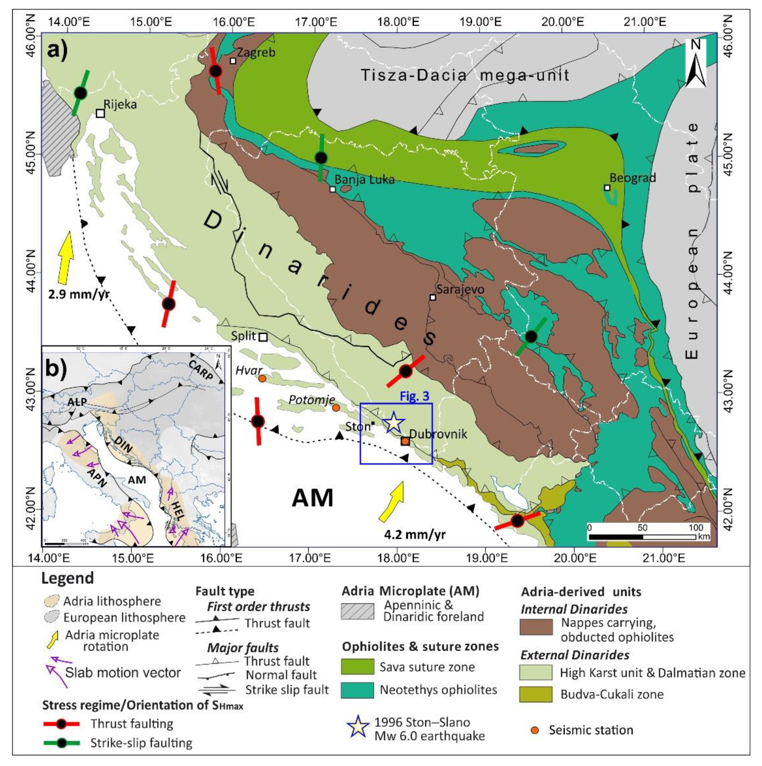
1. Introduction
2. Seismological Observations
- 138,520 observed arrival times of seismic phases for 10,897 earthquakes that occurred between 1 January, 1995 and 5 September, 2018 in the area within the radius of 90 km from the mainshock of the Ston–Slano sequence, based on the seismic data of the Department of Geophysics, Faculty of Science, University of Zagreb (DGFSUZ), and supplemented by arrival times published in the ISC bulletin [21] or in available seismic bulletins from the neighbouring countries. In addition, we have also repicked some onset times from the available seismograms from the analogue and digital seismogram archive of the DGFSUZ, as well as from the international digital seismogram archives [22,23].
- A database of FMS and the corresponding first-motion polarity readings for earthquakes in Croatia and the neighbouring regions since 1910 maintained by the DGFSUZ. Those were either manually read (for all digital seismograms, and for the analogue records obtained at stations of the Croatian Seismograph Network) or adopted from various bulletins and databases. All FMS related to the studied region were rechecked and recomputed using recent crustal models.
- Intensities observed due to the Ston–Slano mainshock in Croatia and Bosnia and Herzegovina from the macroseismic archive of the DGFSUZ. The data on earthquake effects were collected by fieldwork, interviews, questionnaires sent into the greater epicentral area, and from other available sources (e.g., newspaper articles, official damage reports, etc.).
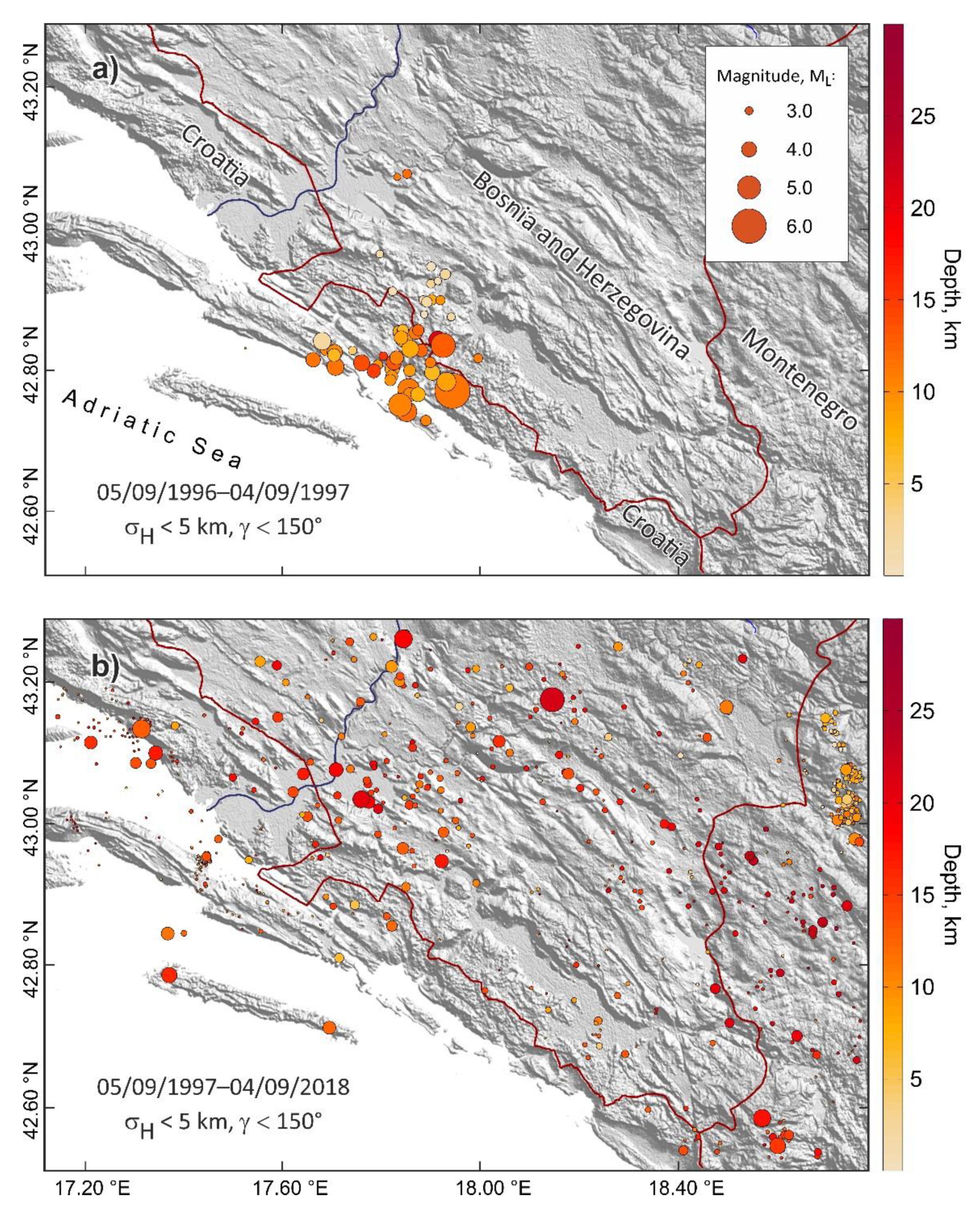
2.1. Earthquake Relocation
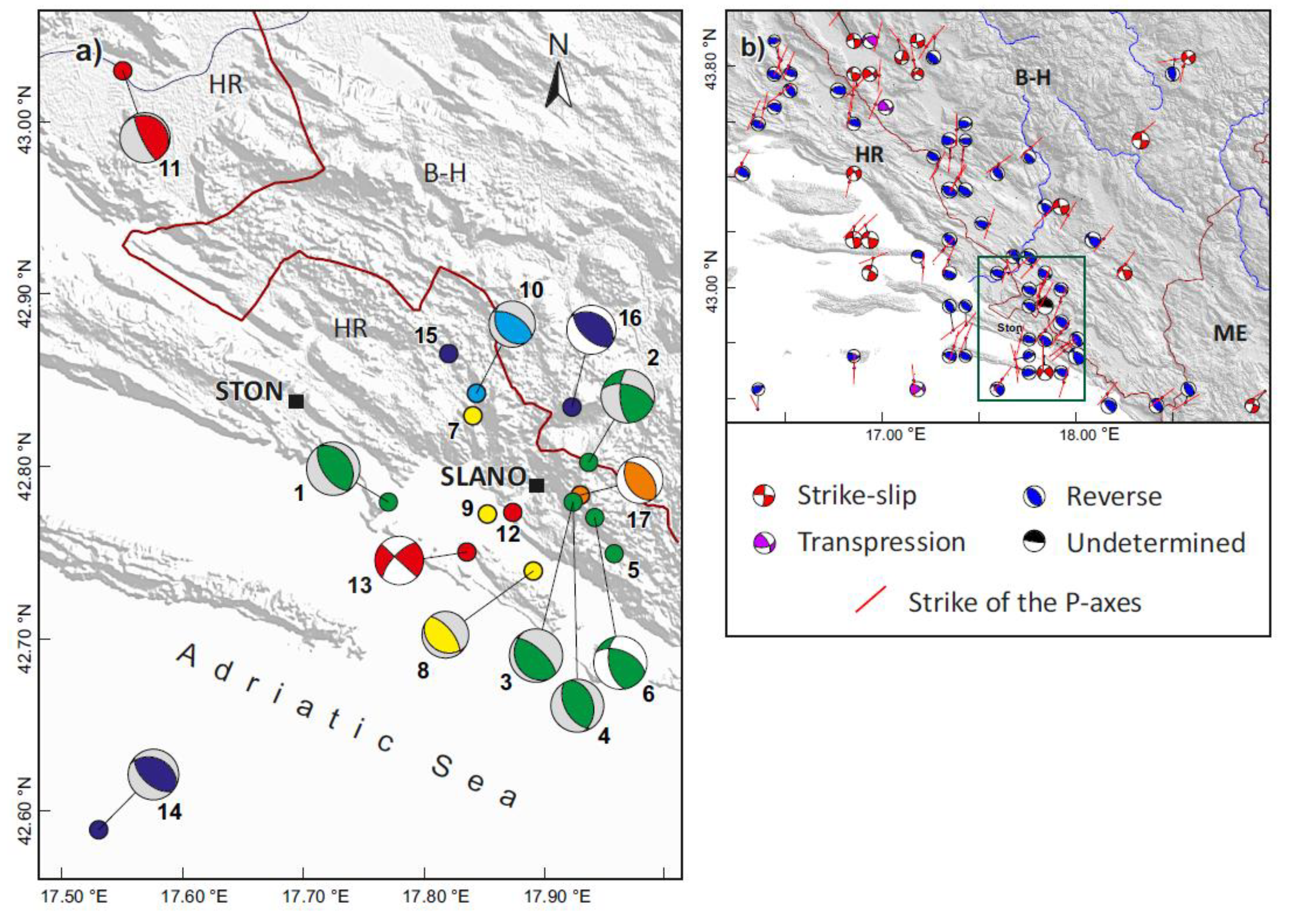
2.2. Fault Mechanism Solutions
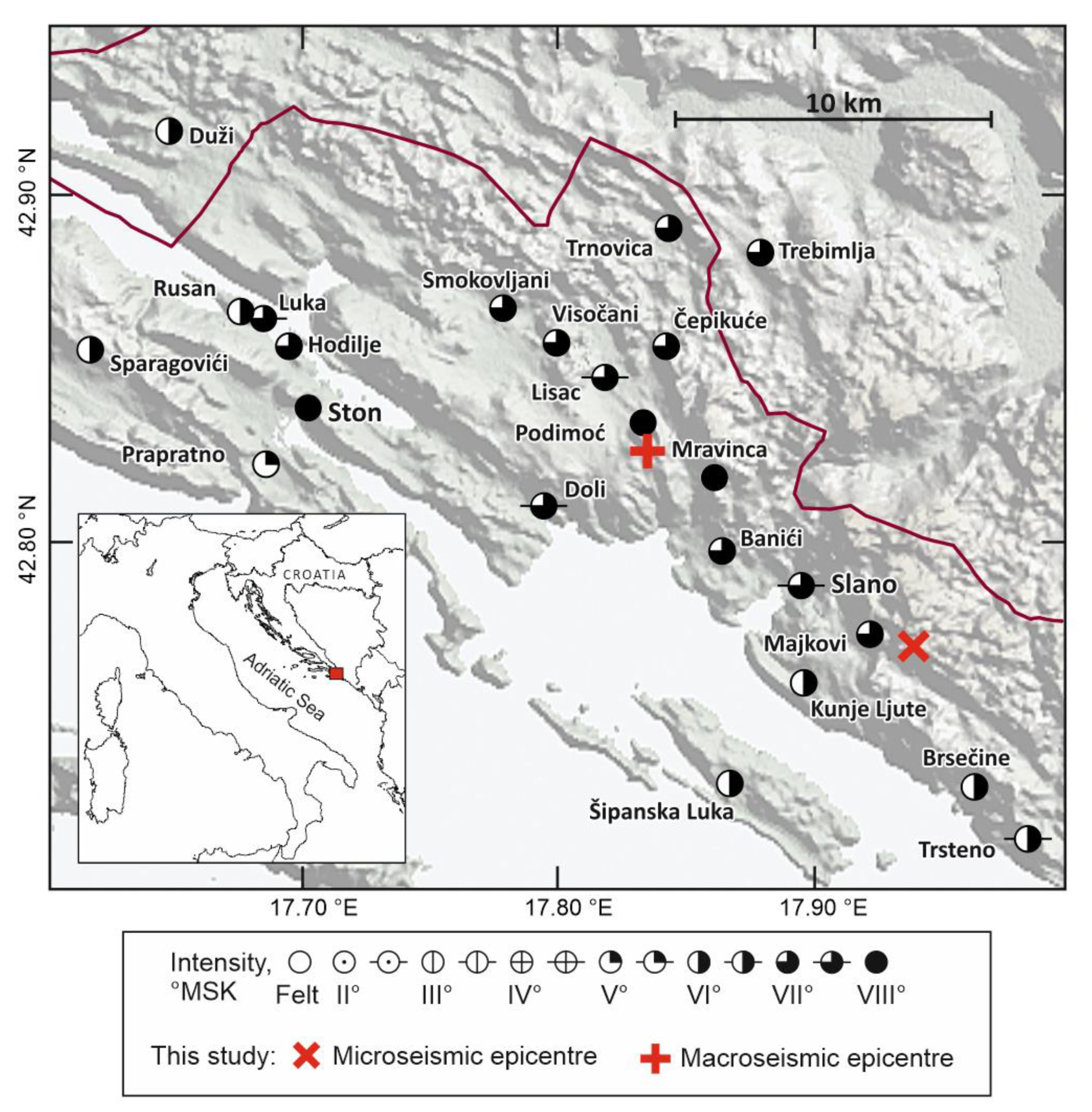
2.3. Inversion of the Macroseismic Field
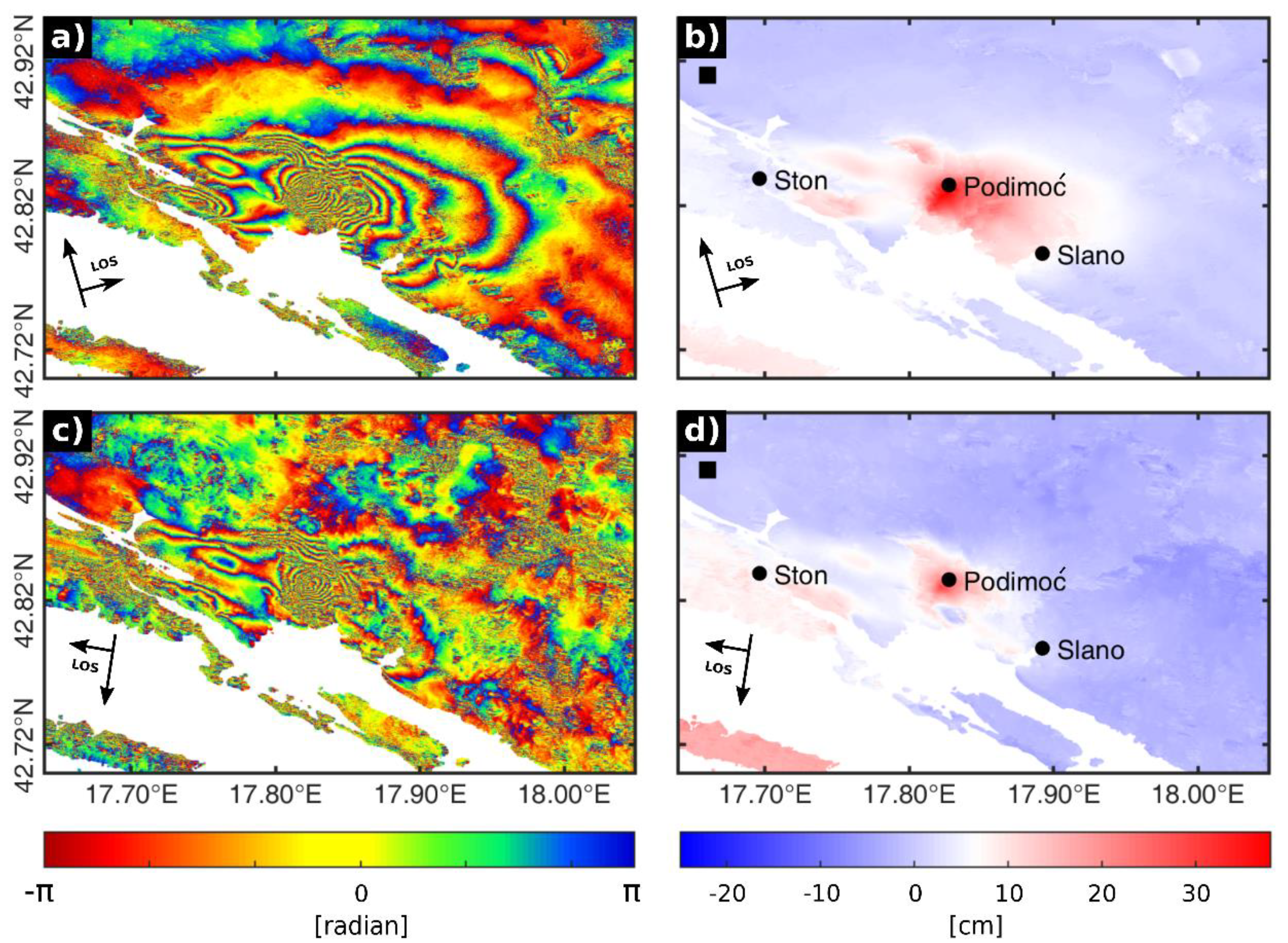
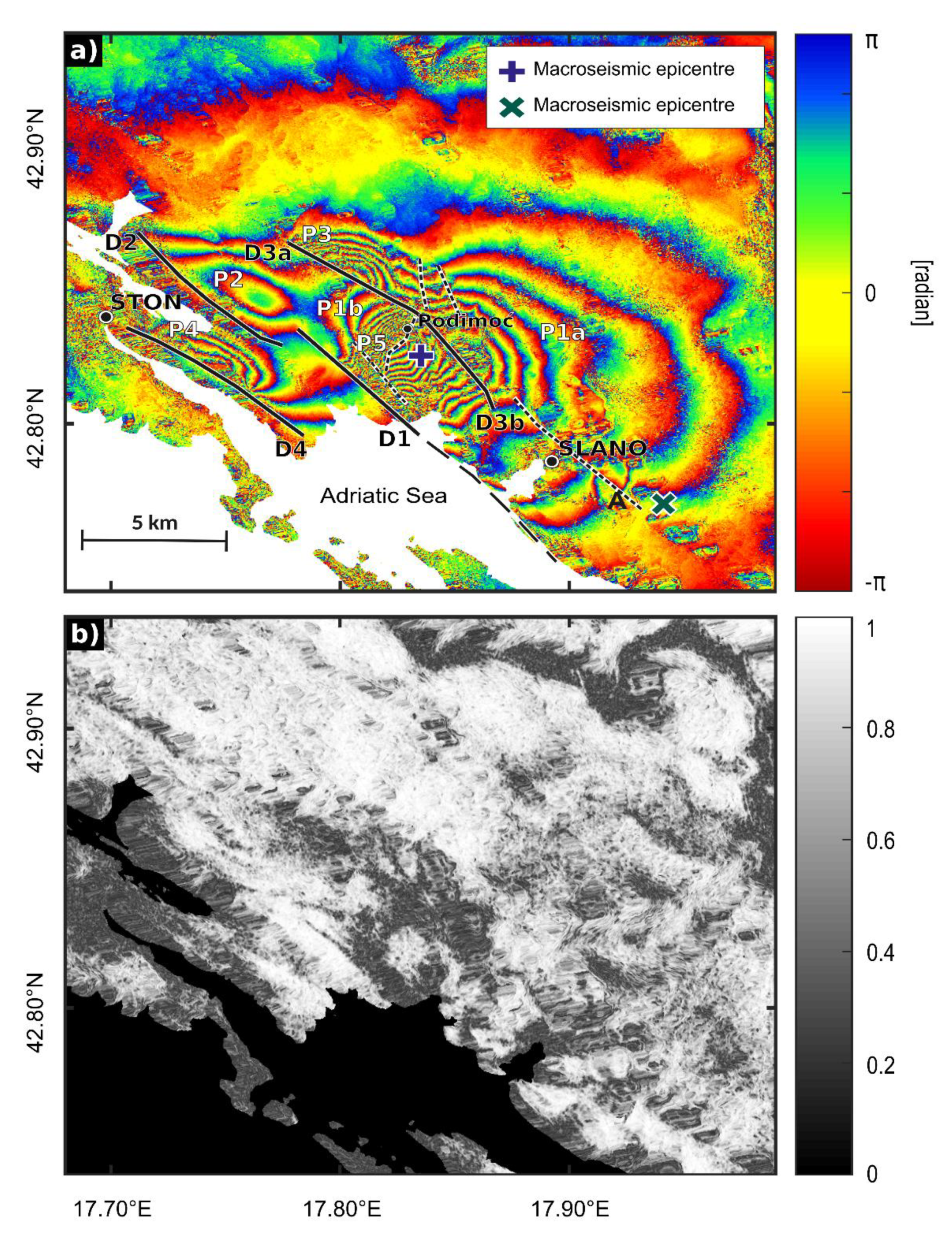
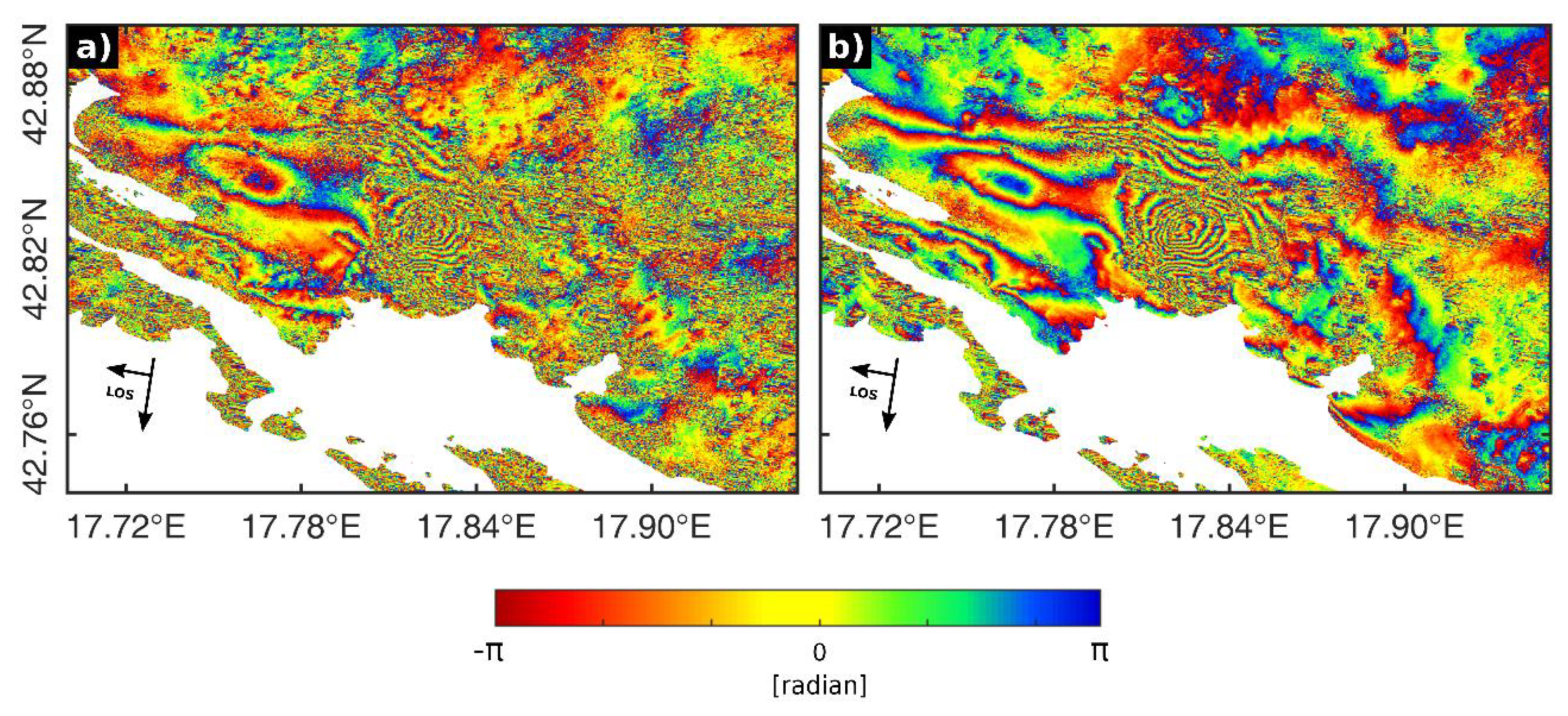
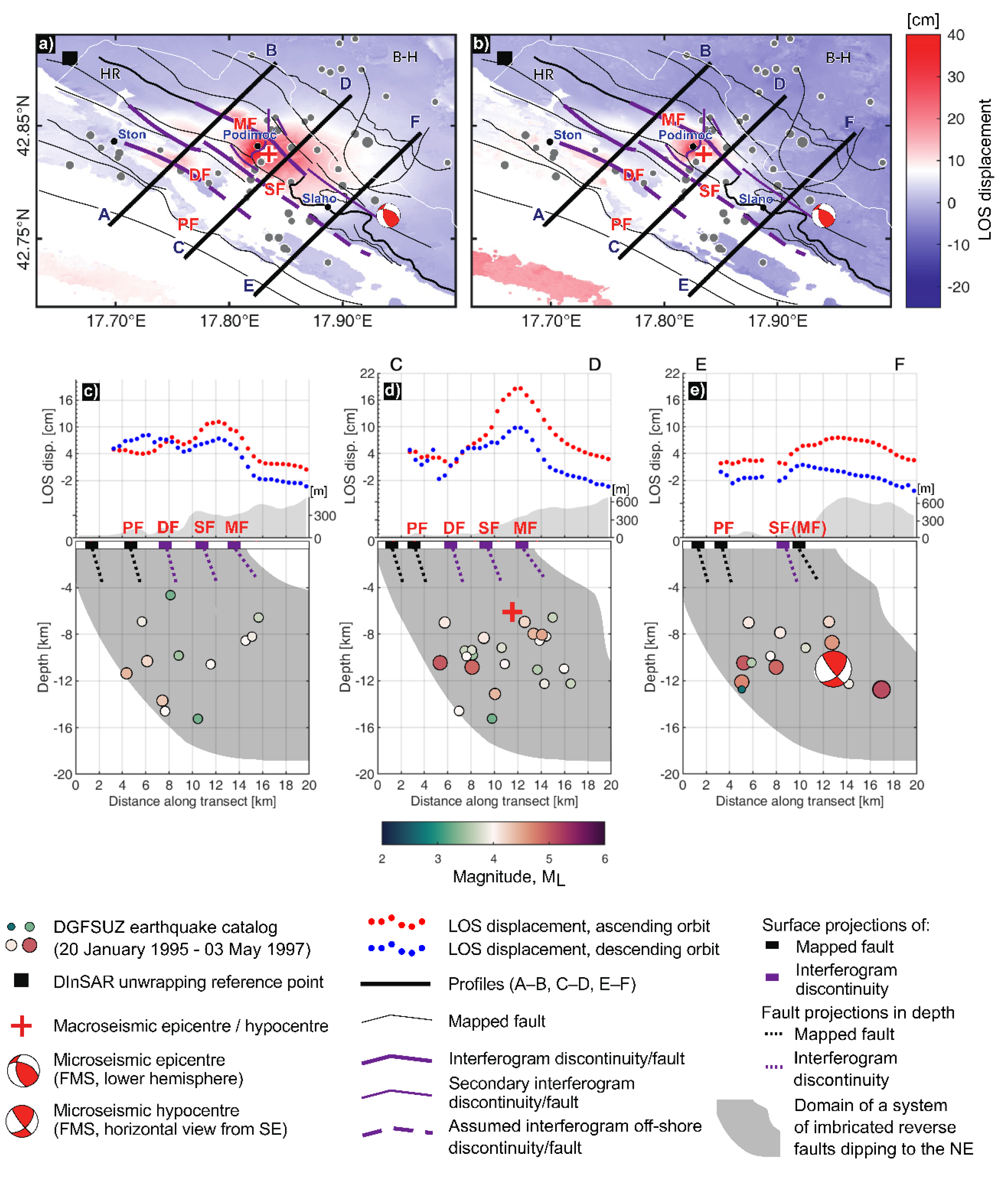
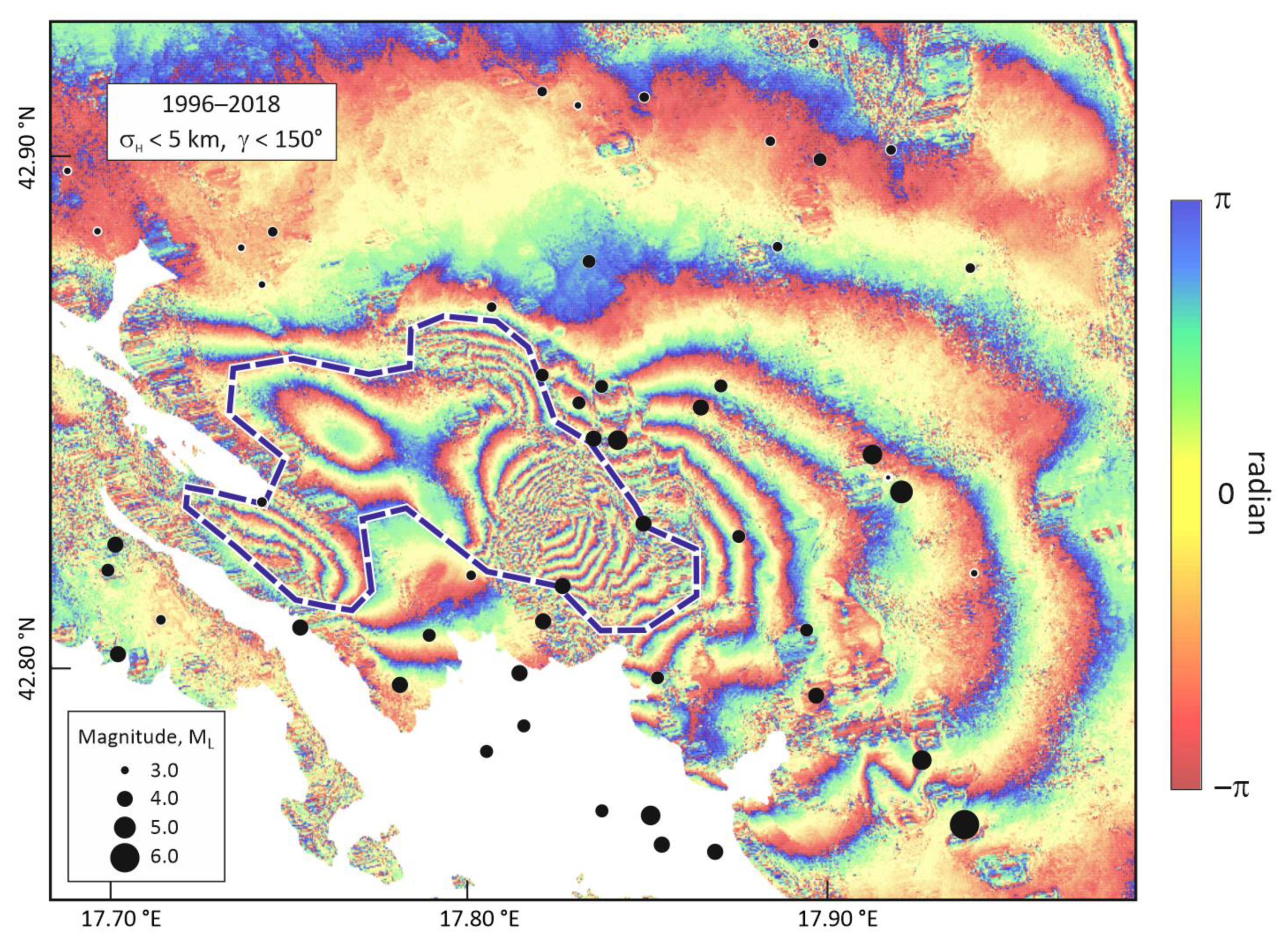
3. DInSAR Observations
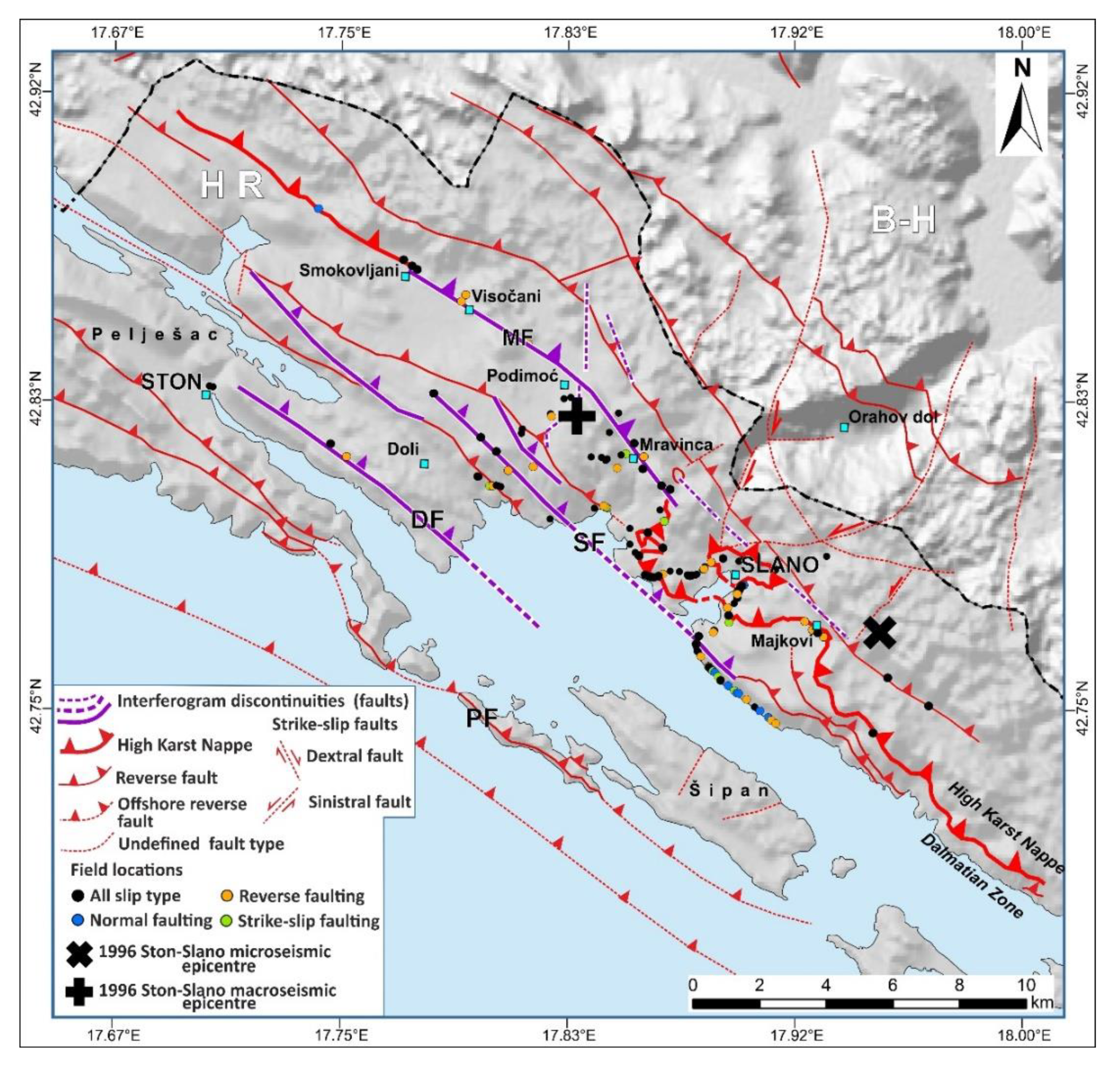
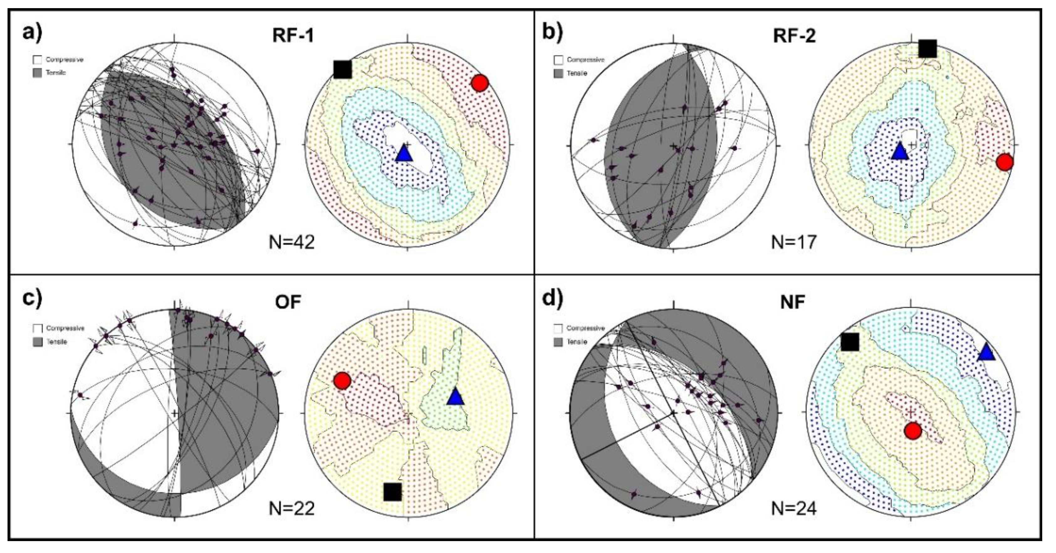
4. Geological Observations
5. Discussion
6. Conclusions
Author Contributions
Funding
Acknowledgments
Conflicts of Interest
References
- Markušić, S.; Herak, D.; Ivančić, I.; Sović, I.; Herak, M.; Prelogović, E. Seismicity of Croatia in the period 1993–1996 and the Ston–Slano earthquake of 1996. Geofizika 1998, 15, 83–101. [Google Scholar]
- Herak, M.; Herak, D.; Markušić, S.; Ivančić, I. Numerical modelling of the Ston–Slano (Croatia) aftershock sequence. Stud. Geophys. Geod. 2001, 45, 251–266. [Google Scholar] [CrossRef]
- Croci, G.; Bonci, A. UNESCO world heritage centre –Mission to Dubrovnik and Ston. Technical Report 1996, 24 pp. Available online: https://whc.unesco.org/document/140421 (accessed on 28 February 2020).
- Herak, M.; Allegretti, I.; Herak, D.; Kuk, K.; Kuk, V.; Marić, K.; Markušić, S.; Stipčević, J. HVSR of ambient noise in Ston (Croatia)—Comparison with theoretical spectra and with the damage distribution after the 1996 Ston–Slano earthquake. Bull. Earthq. Eng. 2010, 8, 483–499. [Google Scholar] [CrossRef]
- University of Zagreb, Macroseismic archives of the Department of Geophysics, Faculty of Science, University of Zagreb, Zagreb, 2020; University of Zagreb: Zagreb, Croatia, 2020.
- Schmid, S.M.; Bernoulli, D.; Fügenschuh, B.; Matenco, L.; Schefer, S.; Schuster, R.; Tischler, M.; Ustaszewski, K. The Alpine–Carpathian–Dinaridic orogenic system: Correlation and evolution of tectonic units. Swiss J. Geosci. 2008, 101, 139–183. [Google Scholar] [CrossRef]
- Ustaszewski, K.; Schmid, S.M.; Lugović, B.; Schuster, R.; Schlategger, U.; Bernoulli, D.; Hottinger, L.; Kounov, A.; Fugenschuh, B.; Schefer, S. Late Cretaceous intra-oceanic magmatism in the internal Dinarides (northern Bosnia and Herzegovina): Implication for the collision of the Adriatic and European Plate. Lithos 2009, 108, 106–125. [Google Scholar] [CrossRef]
- Vlahović, I.; Tišljar, J.; Velić, I.; Matičec, D. Evolution of the Adriatic Carbonate Platform: Palaeogeography, main events and depositional dynamics. Palaeogeogr. Palaeoclimatol. Palaeoecol. 2005, 220, 333–360. [Google Scholar] [CrossRef]
- Schmid, S.M.; Fügenschuh, B.; Kounov, A.; Matenco, L.; Nievergelt, P.; Oberhänsli, R.; Pleuger, J.; Schefer, S.; Schuster, R.; Tomljenović, B.; et al. Tectonic units of the alpine collision zone between Eastern Alps and western Turkey. Gondwana Res. 2020. [Google Scholar] [CrossRef]
- Raić, V.; Papeš, J.; Ahac, A.; Korolija, B.; Borović, I.; Grimani, I.; Marinčić, S. Basic Geological Map of the SFRY, 1:100,000 Scale, Ston Sheet K33-48. Geoinženjering OOUR Institut za geologiju Sarajevo (1972–1980) and Institut za geološka istraživanja Zagreb (1967–1968); Federal Geological Institute: Beograd, Serbia, 1980. [Google Scholar]
- Natević, L.J.; Petrović, V. Basic Geological Map of the SFRY, 1:100,000 Scale, Trebinje Sheet K34-37. Geološki zavod Sarajevo (1963); Federal Geological Institute: Beograd, Serbia, 1967. [Google Scholar]
- D’Agostino, N.; Avallone, A.; Cheloni, D.; D’Anastasio, E.; Mantenuto, S.; Selvaggi, G. Active tectonics of the Adriatic region from GPS and earthquake slip vectors. J. Geophys. Res. B–Solid Earth 2008, 113, B12413. [Google Scholar] [CrossRef]
- Bennett, R.A.; Hreinsdóttir, S.; Buble, G.; Bašić, T.; Bačić, Z.; Marjanović, M.; Casale, G.; Gendaszek, A.; Cowan, D. Eocene to present subduction of southern Adria mantle lithosphere beneath the Dinarides. Geology 2008, 35, 3–6. [Google Scholar] [CrossRef]
- Ivančić, I.; Herak, D.; Markušić, S.; Sović, I.; Herak, M. Seismicity of Croatia in the period 1997–2001. Geofizika 2001, 18–19, 17–29. [Google Scholar]
- Kastelic, V.; Vannoli, P.; Burrato, P.; Fracassi, U.; Tiberti, M.M.; Valensise, G. Seismogenic sources in Adriatic Domain. Mar. Pet. Geol. 2013, 42, 181–213. [Google Scholar] [CrossRef]
- Heidbach, O.; Custodio, S.; Kingdon, A.; Mariucci, M.T.; Montone, P.; Müller, B.; Pierdominici, S.; Rajabi, M.; Reinecker, J.; Reiter, K.; et al. Stress map of the Mediterranean and Central Europe 2016. GFZ Data Serv. 2016. [Google Scholar] [CrossRef]
- Handy, M.; Ustaszewski, K.; Kissling, E. Reconstructing the Alps–Carpathian–Dinarides as a key to understanding switches in subduction polarity, slab gaps and surface motion. Int. J. Earth. Sci. (Geol. Rundsch.) 2014. [Google Scholar] [CrossRef]
- Herak, D.; Herak, M. Focal depth distribution in the Dinara Mt. region, Yugoslavia. Gerlands Beitr. Geophys. 1990, 99, 505–511. [Google Scholar]
- Tomljenović, B.; Herak, M.; Herak, D.; Kralj, K.; Prelogović, E.; Bostjančić, I.; Matoš, B. Active tectonics, seismicity and seismogenic sources of the Adriatic coastal and offshore region of Croatia. In 28 Convegno Nazionale "Riassunti Estesi delle Comunicazioni"; Stella Arti Grafice: Trieste, Italy, 2009; pp. 133–136. [Google Scholar]
- Herak, M.; Herak, D.; Markušić, S. Revision of the earthquake catalogue and seismicity of Croatia, 1908–1992. Terra Nova 1996, 8, 86–94. [Google Scholar] [CrossRef]
- ISC. Bulletin of the International Seismological Centre. Available online: http://www.isc.ac.uk/iscbulletin/search/ (accessed on 28 February 2020).
- EIDA. European Integrated Data Archive. Available online: http://eida.gfz-potsdam.de/webdc3/ (accessed on 28 February 2020).
- IRIS. Incorporated Research Institutions for Seismology. Available online: http://ds.iris.edu/wilber3/find_event (accessed on 28 February 2020).
- Molinari, I.; Morelli, A. EPcrust: A reference crustal model for the European plate. Geophys. J. Int. 2011, 185, 352–364. [Google Scholar] [CrossRef]
- Stipčević, J.; Herak, M.; Molinari, I.; Dasović, I.; Tkalčić, H.; Gosar, A. AlpArray-CASE Working Group and AlpArray Working Group, crustal thickness beneath the Dinarides and surrounding areas from receiver functions. Tectonics 2020, 39, e2019TC005872. [Google Scholar] [CrossRef]
- Herak, M. Hyposearch: An earthquake location program. Comput. Geosci. 1989, 15, 1157–1162. [Google Scholar] [CrossRef]
- Herak, M.; Herak, D. Seismicity and seismic sources in the greater Kvarner–Velebit area, Croatia: Recent advances. In Proceedings of the 5th Regional scientific meeting on quaternary geology dedicated to geohazards, Starigrad-Paklenica, Croatia, 9–10 November 2017; pp. 20–21. [Google Scholar]
- Yang, X.; Bondár, I.; McLaughlin, K.; North, R. Source specific station corrections for regional phases at Fennoscandian stations. Pure Appl. Geophys. 2001, 158, 35–57. [Google Scholar] [CrossRef]
- Materni, V.; Giuntini, A.; Chiappini, S.; Chiappini, M. Relocation of earthquakes by source-specific station corrections in Iran. Bull. Seismol. Soc. Am. 2015, 105, 2498–2509. [Google Scholar] [CrossRef]
- Dziewonski, A.M.; Chou, T.A.; Woodhouse, J.H. Determination of earthquake source parameters from waveform data for studies of global and regional seismicity. J. Geophys. Res. 1981, 86, 2825–2852. [Google Scholar] [CrossRef]
- Ekström, G.; Nettles, M.; Dziewonski, A.M. The global CMT project 2004–2010, Centroid-moment tensors for 13,017 earthquakes. Phys. Earth Planet. Inter. 2012, 200–201, 1–9. [Google Scholar] [CrossRef]
- USGS. U.S. Geological Survey Earthquake Hazards Program. Available online: https://earthquake.usgs.gov/earthquakes/search/https://earthquake.usgs.gov/earthquakes/search/https://earthquake.usgs.gov/earthquakes/search/ (accessed on 28 February 2020).
- GCMT. Global Centroid Moment Tensor Catalog. Available online: https://www.globalcmt.org/CMTsearch.html (accessed on 28 February 2020).
- ISC. International Seismological Centre Global Focal Mechanism Catalogue. Available online: http://www.isc.ac.uk/iscbulletin/search/fmechanisms/ (accessed on 28 February 2020).
- ISC-GEM. International Seismological Centre Global Instrumental Earthquake Catalogue, 2020. Available online: https://doi.org/10.31905/d808b825 (accessed on 28 February 2020).
- RCMT. European-Mediterranean Regional Centroid-Moment Tensors. Available online: http://rcmt2.bo.ingv.it/Italydataset1976-2015.dek (accessed on 28 February 2020).
- Musson, R.M.W. MEEP 2.0 User Guide; Open Report OR/09/045; British Geological Survey: Keyworth, Nottingham, UK, 2009; p. 16. [Google Scholar]
- Herak, M.; Živčić, M.; Sović, I.; Cecić, I.; Dasović, I.; Stipčević, J.; Herak, D. Historical seismicity of the Rijeka region (NW External Dinarides, Croatia)–Part II: The Klana earthquakes of 1870. Seismol. Res. Lett. 2018, 89, 1524–1536. [Google Scholar] [CrossRef]
- Herak, D.; Živčić, M.; Vrkić, I.; Herak, M. The Međimurje (Croatia) earthquake of 1738. Seismol. Res. Lett. 2020, 91, 1042–1056. [Google Scholar] [CrossRef]
- Massonnet, D.; Rossi, M.; Carmona, C.; Adragna, F.; Peltzer, G.; Feigl, K.; Rabaute, T. The displacement field of the Landers earthquake mapped by radar interferometry. Nature 1993, 364, 138–142. [Google Scholar] [CrossRef]
- Rosen, P.A.; Gurrola, E.; Sacco, G.F.; Zebker, H. The InSAR scientific computing environment. In Proceedings of the EUSAR. 9th European Conference on Synthetic Aperture Radar, Nuremberg, Germany, 23–26 April 2012; pp. 730–733. [Google Scholar]
- Farr, T.G.; Rosen, P.A.; Caro, E.; Crippen, R.; Duren, R.; Hensley, S.; Kobrick, M.; Paller, M.; Rodriguez, E.; Roth, L.; et al. The shuttle radar topography mission. Rev. Geophys. 2007, 45, RG2004. [Google Scholar] [CrossRef]
- Massonnet, D.; Feigl, K.L. Discrimination of geophysical phenomena in satellite radar interferograms. Geophys. Res. Lett. 1995, 22, 1537–1540. [Google Scholar] [CrossRef]
- Hanssen, R.F. Radar Interferometry: Data Interpretation and Error Analysis; Springer Science & Business Media: Berlin/Heidelberg, Germany, 2001; Volume 2. [Google Scholar]
- Scharoo, R.; Visser, P.N.A.M.; Mets, G.J. Precise orbit determination and gravity field improvement for the ERS satellites. J. Geophys. Res. 1998, 88, 4984–4996. [Google Scholar] [CrossRef]
- Goldstein, R.M.; Werner, C.L. Radar interferogram filtering for geophysical applications. Geophys. Res. Lett. 1998, 25, 4035–4038. [Google Scholar] [CrossRef]
- Chen, C.W.; Zebker, H.A. Two-dimensional phase unwrapping with use of statistical models for cost functions in nonlinear optimization. J. Opt. Soc. Am. 2001, 18, 338–351. [Google Scholar] [CrossRef]
- Ortner, H.; Reiter, F.; Acs, P. Easy handling of tectonic data: The programs Tectonic VB for Mac and Tectonics FP for Windows TM. Comput. Geosci. 2002, 28, 1193–1200. [Google Scholar] [CrossRef]
- Turner, F.J. Nature and dynamic interpretation of deformation lamellae in calcite of three marbles. Am. J. Sci. 1953, 251, 276–298. [Google Scholar] [CrossRef]
- Marrett, R.; Allmendinger, R.W. Kinematic analysis of fault-slip data. J. Struct. Geol. 1990, 12, 973–986. [Google Scholar] [CrossRef]
- Angelier, J.; Mechler, P. Sur une méthode graphique de recherche des contraintes principales également utilisable en tectonique et en séismologie: La méthode des dièdres droits. Bull. Soc. Géol. Fr. 1977, 19, 1309–1318. [Google Scholar] [CrossRef]
- Wells, D.L.; Coppersmith, K.J. New empirical relationships among magnitude, rupture length, rupture width, rupture area, and surface displacement. Bull. Seismol. Soc. Am. 1994, 84, 974–1002. [Google Scholar]
- Funning, G.J.; Garcia, A. A systematic study of earthquake detectability using Sentinel-1 Interferometric Wide-Swath data. Geophys. J. Int. 2019, 216, 332–349. [Google Scholar] [CrossRef]
- Ross, Z.E.; Idini, B.; Jia, Z.; Stephenson, O.L.; Zhong, M.; Wang, X.; Zhan, Z.; Simons, M.; Fielding, E.J.; Yun, S.-H.; et al. Hierarchical interlocked orthogonal faulting in the 2019 Ridgecrest earthquake sequence. Science 2019, 366, 346–351. [Google Scholar] [CrossRef]
- Chounet, M.; Vallée, M.; Causse, M.; Courboulex, F. Global catalog of earthquake rupture velocities shows anticorrelation between stress drop and rupture velocity. Tectonophysics 2018, 733, 148–158. [Google Scholar] [CrossRef]


| No. | Date | Time, DT (s)1 | Lat., °N | Lon., °E | C, E1 | Depth, km | Mag. | ϕ1°, δ1°, λ1° ϕ2°, δ2°, λ2° (BDC or FMS) 1 | Source 2 |
|---|---|---|---|---|---|---|---|---|---|
| 1 | Mainshock 5 September, 1996 | 20:44:17.3 DT = 8.1 s | 42.78 | 17.77 | C | 15.0 | Mw 6.0, mb 5.6, MS 6.0 | 328, 32, 92 146, 58, 89 (BDC) | GCMT |
| 2 | 20:44:09 | 42.80 | 17.94 | E | 10.0 | Mwc 6.0 | 285, 55, 30 177, 66, 141 (FMS) | USGS | |
| 3 | 20:44:11.3 | 42.78 | 17.92 | E | 13.3 | Mw 5.9 | 345, 40, 102 150, 52, 80 (FMS) | ISC | |
| 4 | 20:44:11.3 | 42.78 | 17.92 | E | 13.3 | Mw 6.0, mb 5.6, MS 6.0 | 312, 69, 82 153, 23, 110 (FMS) | ISC | |
| 5 | 20:44:11 | 42.75 | 17.96 | E | 12.5 | Mw 6.0 | – | ISCGEM | |
| 6 | 20:44:07.9 | 42.77 ± 5 km | 17.94 ± 5 km | E | 11.4 ± 5 | ML 6.0 | 293, 53, 47 170, 54, 132 (FMS) | This study | |
| 7 | Aftershock 5 September, 1996 | 21:43:31.1 | 42.83 | 17.84 | E | 10.0 | mb 4.9 | – | RCMT (from PDE) |
| 8 | 21:43:34.6 DT = 3.5 s | 42.74 | 17.89 | C | 15.0 | Mw 4.6 | 321, 66 100 119, 26, 70 (BDC) | RCMT (from PDE) | |
| 9 | 21:43:30.3 | 42.77 ± 4 km | 17.85 ± 4 km | E | 10.8 ± 2 | ML 4.9 | – | This study | |
| 10 | Aftershock 7 September, 1996 | 05:45:32.4 | 42.85 | 17.84 | E | 8.1 | ML 4.5 | 301, 59, 77 145,33, 111 (FMS) | This study |
| 11 | Aftershock 9 September, 1996 | 15:57:08.7 DT = 3.6 s | 43.03 | 17.55 | C | 15.0 | Mw 5.3, mb 4.8, MS 5.0 | 301, 13, 58 154, 79, 97 (BDC) | GCMT |
| 12 | 15:57:05 | 42.77 | 17.873 | E | 10.0 | Mwc 5.3 | – | USGS | |
| 13 | 15:57:04.6 | 42.75± 2 km | 17.83± 2 km | E | 10.5± 2 | ML 5.0 | 223, 69, 1 133, 89, 159 (FMS) | This study | |
| 14 | Aftershock 17 September, 1996 | 13:45:27.9 DT = 5.1 s | 42.59 | 17.53 | C | 15.0 | Mw 5.4, mb 5.4, MS 5.1 | 295, 35, 76 132, 56, 99 (BDC) | GCMT |
| 15 | 13:45:22 | 42.87 | 17.82 | E | 10.0 | Mwc 5.4 | – | USGS | |
| 16 | 13:45:22.1 | 42.83 ± 2 km | 17.92 ± 2 km | E | 12.8 ± 1 | ML 5.1 | 299, 33, 77 134, 58, 98 (FMS) | This study | |
| 17 | Aftershock 20 October, 1996 | 15:00:01.7 | 42.78 ± 1 km | 17.93 ± 1 km | E | 8.7 ± 2 | ML 4.6 | 319, 47, 83 149, 43, 97 (FMS) | This study |
| Sat. | Orbit Direction | Track | Master Image (yr/mm/dd) | Slave Image (yr/mm/dd) | Bperp (m) | Btemp (days) | Hamb (m) |
|---|---|---|---|---|---|---|---|
| ERS-2 | Descending | 451 | 09/08/1996 | 16/051997 | –59 | 280 | 158 |
| ERS-2 | Ascending | 501 | 06/11/1995 | 01/091997 | –17 | 665 | 547 |
| Fault group | Fault subset | No. of fault data | Dip azimuth (°) | Dip angle (°) | Pitch (°) | Fault type | Striation | P-axis | T-axis | |||
|---|---|---|---|---|---|---|---|---|---|---|---|---|
| Trend (°) | Plunge (°) | Trend (°) | Plunge (°) | Trend (°) | Plunge (°) | |||||||
| RF-1 | RF-1a | 27 | 44 | 51 | 69 | R | 113 | 49 | 50 | 8 | 205 | 82 |
| RF-1b | 15 | 216 | 32 | 69 | 237 | 49 | ||||||
| RF-2 | RF-2a | 11 | 95 | 52 | 57 | R | 139 | 46 | 100 | 8 | 247 | 80 |
| RF-2b | 6 | 291 | 32 | 51 | 218 | 46 | ||||||
| OF | OFa | 16 | 86 | 88 | 3 | O-S | 138 | 4 | 296 | 30 | 70 | 50 |
| OFb | 6 | 184 | 20 | 0 | S-S | 100 | 1 | |||||
| NF | NFa | 18 | 41 | 51 | 69 | N | 85 | 51 | 173 | 75 | 51 | 08 |
| NFb | 6 | 243 | 4 | 55 | 221 | 49 | ||||||
© 2020 by the authors. Licensee MDPI, Basel, Switzerland. This article is an open access article distributed under the terms and conditions of the Creative Commons Attribution (CC BY) license (http://creativecommons.org/licenses/by/4.0/).
Share and Cite
Govorčin, M.; Herak, M.; Matoš, B.; Pribičević, B.; Vlahović, I. Constraints on Complex Faulting during the 1996 Ston–Slano (Croatia) Earthquake Inferred from the DInSAR, Seismological, and Geological Observations. Remote Sens. 2020, 12, 1157. https://doi.org/10.3390/rs12071157
Govorčin M, Herak M, Matoš B, Pribičević B, Vlahović I. Constraints on Complex Faulting during the 1996 Ston–Slano (Croatia) Earthquake Inferred from the DInSAR, Seismological, and Geological Observations. Remote Sensing. 2020; 12(7):1157. https://doi.org/10.3390/rs12071157
Chicago/Turabian StyleGovorčin, Marin, Marijan Herak, Bojan Matoš, Boško Pribičević, and Igor Vlahović. 2020. "Constraints on Complex Faulting during the 1996 Ston–Slano (Croatia) Earthquake Inferred from the DInSAR, Seismological, and Geological Observations" Remote Sensing 12, no. 7: 1157. https://doi.org/10.3390/rs12071157
APA StyleGovorčin, M., Herak, M., Matoš, B., Pribičević, B., & Vlahović, I. (2020). Constraints on Complex Faulting during the 1996 Ston–Slano (Croatia) Earthquake Inferred from the DInSAR, Seismological, and Geological Observations. Remote Sensing, 12(7), 1157. https://doi.org/10.3390/rs12071157