Spatio-Temporal Sub-Pixel Land Cover Mapping of Remote Sensing Imagery Using Spatial Distribution Information From Same-Class Pixels

Abstract

The generation of land cover maps with both fine spatial and temporal resolution would aid the monitoring of change on the Earth’s surface. Spatio-temporal sub-pixel land cover mapping (STSPM) uses a few fine spatial resolution (FR) maps and a time series of coarse spatial resolution (CR) remote sensing images as input to generate FR land cover maps with a temporal frequency of the CR data set. Traditional STSPM selects spatially adjacent FR pixels within a local window as neighborhoods to model the land cover spatial dependence, which can be a source of error and uncertainty in the maps generated by the analysis. This paper proposes a new STSPM using FR remote sensing images that pre- and/or post-date the CR image as ancillary data to enhance the quality of the FR map outputs. Spectrally similar pixels within the locality of a target FR pixel in the ancillary data are likely to represent the same land cover class and hence such same-class pixels can provide spatial information to aid the analysis. Experimental results showed that the proposed STSPM predicted land cover maps more accurately than two comparative state-of-the-art STSPM algorithms.

1. Introduction

Land cover change plays a major role in environmental processes and patterns such as the global carbon cycle and ecosystem diversity [1,2]. Optical remote sensing provides the opportunity to monitor and map the land cover transition trajectories from space with different spatial and temporal resolutions. Coarse spatial resolution (CR) remote sensing imagery such as the Moderate Resolution Imaging Spectroradiometer (MODIS) have a short revisiting period that can be used to monitor land cover with a high temporal frequency but lack spatial detail. The relatively large size of the pixels in such CR imagery often results in a large proportion of the image being composed of mixed pixels which can degrade the ability to accurately map the land cover [3]. The mixed pixel problem can be reduced through the use of spectral unmixing or soft classification analysis that allow for multiple class membership [4]. Typically, the output of an unmixing or soft classification is a set of class fraction images that represent the proportional cover of the classes in the area represented by CR pixels. However, a limitation of spectral unmixing is that the spatial distribution of each class within the CR pixels is still unknown. The latter may, however, be estimated using super-resolution mapping techniques such as sub-pixel mapping (SPM).

SPM is a technique that predicts a land cover map with a finer spatial resolution than the image from which it is derived [5,6]. The SPM analysis typically uses the sub-pixel scale land cover information contained in class fraction images to locate the classes geographically in the area represented by CR pixels. A range of SPM algorithms has been developed [7,8,9,10,11,12] and the approach has been applied to data sets ranging from a single, mono-temporal, CR image to spatio-temporal SPM that uses a time series of CR images [13,14]. In the latter, the analysis may also be enhanced through the integration of information from a few fine spatial resolution (FR) land cover maps, if available, which enable the generation of FR land cover maps at the temporal frequency of the CR imagery [15]. For studies of land cover change, such spatio-temporal SPM (STSPM) is more appropriate than SPM as the incorporated FR maps can greatly reduce the uncertainty in modeling FR land cover temporal change trajectories [13,15]. STSPM has been applied in numerous studies to produce FR maps that facilitate the monitoring of land cover change [13,14,15,16,17,18,19,20] and the filling of gaps in time series products such as maps of annual forest cover obtained from PALRSAR/PALSAR2 [21].

Although a range of STSPM algorithms has been developed in recent years, limitations still exist in accurately predicting the sub-pixel scale land cover map. The limitation is mainly because the land cover spatial distribution model adopted in STSPM is relatively simple, which makes it difficult to represent the real-world complex spatial distribution of various land covers [5]. The most popular land cover spatial distribution model used in SPM and STSPM is the spatial dependence model, which aims to maximize the spatial dependence between neighboring FR pixels, based on the assumption that spatially adjacent objects are more alike than those that are far apart [5]. However, the spatial dependence model is most suitable when the object of interest is larger than the CR pixel size. Objects are, however, often smaller than the CR pixel size and the aim of SPM is to represent the land cover mosaic at a sub-pixel scale. Furthermore, using the spatial dependence model in SPM and STSPM usually produces inappropriate smoothed boundaries between classes [13,22].

One way to reduce errors in STSPM is to incorporate additional ancillary data to constrain the analysis in order to enhance the quality of the map generated from it. A range of ancillary data sets may be used. For example, studies have used the digital elevation model (DEM) [23], vector boundaries [24], and points-of-interest (POI) [25] to refine the result from SPM. However, in such studies it is typically assumed that the land cover is the same at the time of acquisition of both the ancillary data and the CR image. This assumption may be untenable for environments that experience relatively abrupt land cover change. A temporally dense FR data set would be attractive in STSPM for areas that experience abrupt land cover change. It is important that the ancillary data should be acquired temporally close to the date of the map to be predicted and that the ancillary data should be temporally updated.

In STSPM, the FR maps used to inform the analysis are usually produced from FR remote sensing images. These FR images could, however, also be used as a source of additional ancillary data for use in STSPM. In the ancillary FR images, the local similar pixels are likely from the same land cover class. For each FR pixel, a number of similar FR pixels within a local window could be extracted that have the most similar spectral values to the target pixel in the ancillary FR images. The spatial distribution of the local similar pixels could represent the spatial distribution information about the same-class pixels to the target FR pixel within the local window. Since the same-class pixels are extracted from FR images, they can indicate detailed land cover spatial distribution information within the CR pixels, which can be used in combination with the spatial dependence model in STSPM to avoid producing over-smoothed boundaries between land cover patches. The same-class pixels are extracted from the ancillary FR images which are temporally updated in a high frequency, and the effect of abrupt change between the dates of ancillary data and the map to be predicted is expected to be minimized.

This paper proposed a novel STSPM that uses not only FR land cover maps but also FR remote sensing images as ancillary data to help the analysis. Unlike traditional STSPMs that only use FR land cover maps as ancillary data and use spatial dependence models to characterize the land cover spatial distribution, the proposed method also incorporates same-class pixels from the ancillary FR images to assist the prediction of land cover spatial distributions at the FR scale. The proposed same-class pixels-based STSPM model, i.e., SCPSM, was assessed in three experiments with different land cover change scenarios. The first experiment focused on land cover changes of a spatially heterogeneous region in which six land cover classes were present. The second experiment focused on land cover change caused by a forest fire. The third experiment focused on deforestation due to forest clearance. The first and second experiments used resampled remote sensing images as the CR image to exclude errors such as misregistration, and the third experiment used a real MODIS MCD43A4 image as the CR image and Landsat as the source FR images. The proposed SCPSM was compared with two state-of-the-art STSPM algorithms.

2. Methods

2.1. The Scheme of SCPSM

STSPM predicts the FR land cover map ${\mathrm{X}}_{tp}^{FR}$ at the time of CR image ${\mathit{y}}_{tp}^{CR}$ acquisition t_p, using FR land cover ${\mathrm{X}}_{t0}^{FR}$ and ${\mathrm{X}}_{tn}^{FR}$ at observation times t₀ and t_n as input (t₀<t_p<t_n). SCPSM also inputs the FR images ${\mathit{y}}_{t0}^{FR}$ and ${\mathit{y}}_{tn}^{FR}$ at observation times t₀ and t_n. The input CR image ${\mathit{y}}_{tp}^{CR}$ contains I×J pixels and B^CR spectral bands. The input FR maps ${\mathrm{X}}_{t0}^{FR}$ and ${\mathrm{X}}_{tn}^{FR}$ contain I×s×J×s pixels where s is the scale factor between the CR and FR pixels, and contain C land cover classes. Each CR pixel contains s×s FR pixels. 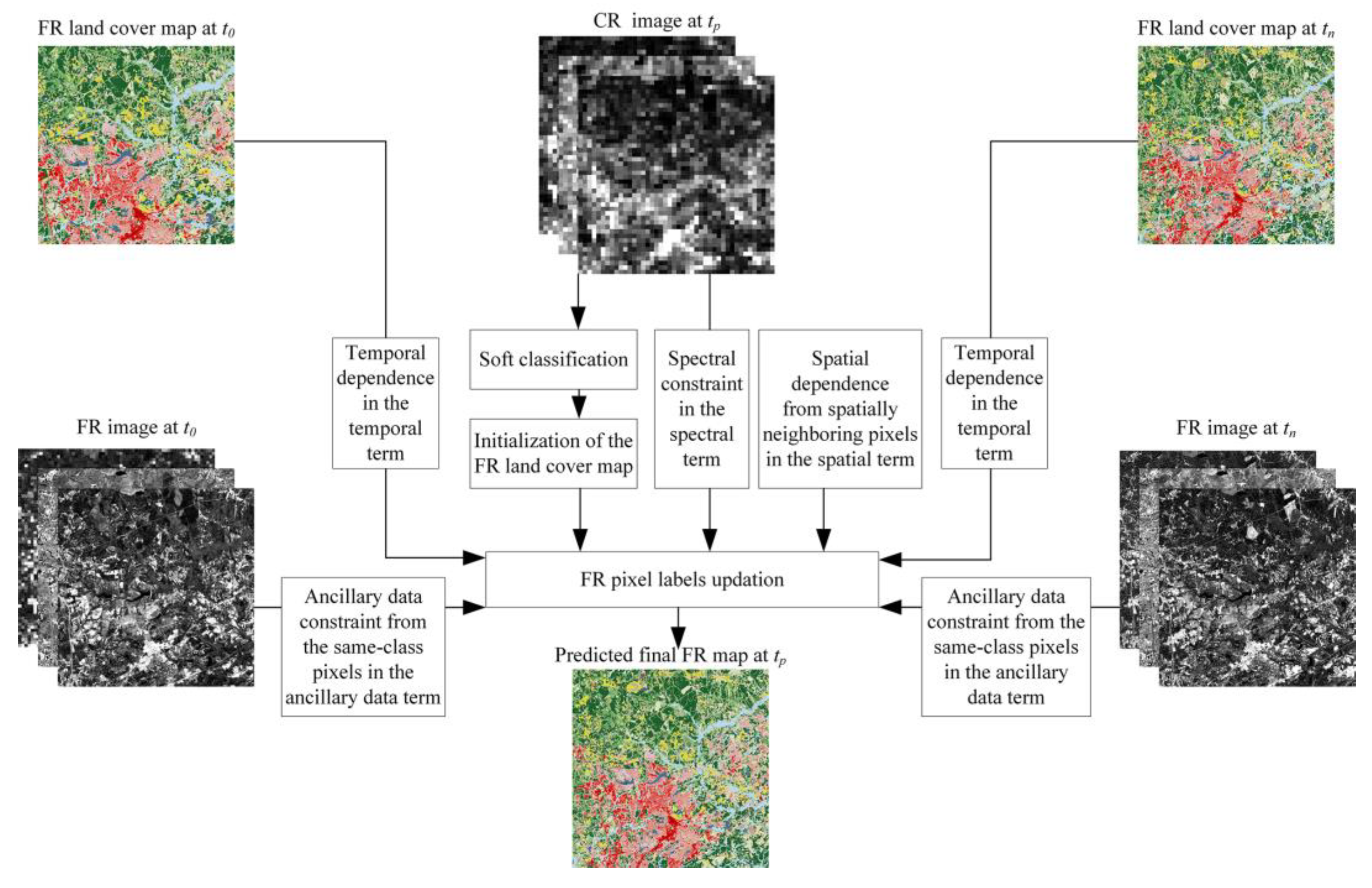The FR images ${\mathit{y}}_{t0}^{FR}$ and ${\mathit{y}}_{tn}^{FR}$ contain I×s×J×s pixels and B^FR spectral bands. The estimation of FR map using STSPM is equivalent to minimizing the energy function in Equation (1):

$$\begin{array}{ll}f\left({\mathrm{X}}_{tp}^{FR}\right)& ={\lambda }^{spatial}\cdot U^{spatial}({\mathrm{X}}_{tp}^{FR})+{\lambda }^{ancillary}\cdot U^{ancillary}({\mathrm{X}}_{tp}^{FR}|{\mathit{y}}_{t0}^{FR},{\mathit{y}}_{tn}^{FR})\\ & +{\lambda }^{temporal}\cdot U^{temporal}({\mathrm{X}}_{tp}^{FR}|{\mathrm{X}}_{t0}^{FR},{\mathrm{X}}_{tn}^{FR})+U^{spectral}({\mathit{y}}_{tp}^{CR}|{\mathrm{X}}_{tp}^{FR})\end{array}$$

(1)

where f(${\mathrm{X}}_{tp}^{FR}$) is the objective function, U^spatial(${\mathrm{X}}_{tp}^{FR}$) is the spatial term, U^ancillary(${\mathrm{X}}_{tp}^{FR}$|${\mathit{y}}_{t0}^{FR}$,${\mathit{y}}_{tn}^{FR}$) is the ancillary data term, U^temporal(${\mathrm{X}}_{tp}^{FR}$|${\mathrm{X}}_{t0}^{FR}$,${\mathrm{X}}_{tn}^{FR}$) is the temporal term, and U^spectral(${\mathit{y}}_{tp}^{CR}$|${\mathrm{X}}_{tp}^{FR}$) is the spectral term, respectively. λ^spatial, λ^ancillary, and λ^temporal are the weights of the spatial, ancillary data and temporal terms, respectively. The flow chart of SCPSM is in Figure 1.

2.2. Spatial Term

The STSPM spatial term aims to encode the land cover spatial distribution prior information in predicting the FR map ${\mathrm{X}}_{tp}^{FR}$. The spatial dependence model is used in this paper, and the class label of the target FR pixel is dependent on its spatially neighboring FR pixels in a local window [22]. Assume N^spatial(a_ijk) is the set of FR spatially neighboring pixels that includes all FR pixels inside a square window whose center is a_ijk, and a_l is a spatially neighboring pixel of a_ijk in N^spatial(a_ijk). The size of the neighborhood N^spatial(a_ijk) is W^spatial, and N^spatial(a_ijk) contains a total of L FR pixels, excluding the central pixel (L = W^spatial×W^spatial−1). Figure 2a shows an example of the selected FR spatially neighboring pixels within a 3×3 local window. The spatial energy from the spatially neighboring pixels for the FR pixel a_ijk is calculated as:

$$U_{ijk}^{spatial}={\displaystyle \sum _{l=1}^L{w}_l^{spatial}\times \delta \left(c(a_{ijk}),c(a_l)\right)}$$

(2)

where c(a_l) is the land cover class label for FR pixel a_l, and δ(c(a_ijk),c(a_l)) equals 1 if c(a_ijk) and c(a_l) are the same and 0 otherwise. $w_l^{spatial}$ is the weight of FR spatially neighboring pixel that is calculated as:

$$w_l^{spatial}=\left(1/d\left(a_{ijk},a_l\right)\right)/{\displaystyle \sum _{l=1}^L\left(1/d\left(a_{ijk},a_l\right)\right)}$$

(3)

where d(a_ijk,a_l) is the Euclidean distance between a_ijk and a_l.

The contribution of the spatial term from all FR pixels is calculated as:

$$U^{spatial}({\mathrm{X}}_{tp}^{FR})={\displaystyle \sum _{i=1}^I{\displaystyle \sum _{j=1}^J{\displaystyle \sum _{k=1}^{s^2}\left(-1\times U_{ijk}^{spatial}\right)}}}.$$

(4)

2.3. Ancillary Data Term

In the ancillary data term, the same-class FR pixels extracted from the ancillary FR images are used in predicting the FR pixel labels, and the class label of the target FR pixel is dependent on its same-class FR pixels within a local window. The same-class FR pixels are selected according to the smallest spectral difference between the target FR pixel and the FR pixels within the local window in the ancillary FR images. Figure 2b–c shows the schematic diagram of the selection of FR same-class pixels within a local window from ${\mathit{y}}_{t0}^{FR}$ and ${\mathit{y}}_{tn}^{FR}$, respectively. For a target FR pixel a_ijk, a local window centered at a_ijk is first defined (marked as dashed lines in Figure 2b–d). The local window size is W^ancillary. Then the spectral difference between a_ijk and a FR pixel a_m within the local window at time t₀ and t_n is calculated as:

$$S_{m,t_0}={\displaystyle \sum _{b=1}^{B^{FR}}\left(\left|y_{ijk,b,t_0}-y_{m,b,t_0}\right|/y_{ijk,b,t_0}\right)}$$

(5)

$$S_{m,t_n}={\displaystyle \sum _{b=1}^{B^{FR}}\left(\left|y_{ijk,b,t_n}-y_{m,b,t_n}\right|/y_{ijk,b,t_n}\right)}$$

(6)

where y_ijk,b,t0 and y_m,b,t0 are the spectral values of FR pixels a_ijk and a_m in the FR image ${\mathit{y}}_{t0}^{FR}$, and y_ijk,b,tn and y_m,b,tn are the spectral values of FR pixels a_ijk and a_m in the FR image ${\mathit{y}}_{tn}^{FR}$. A number of M FR pixels with the smallest spectral difference at time t₀ and t_n are selected as same-class FR neighboring pixels for the target FR pixel a_ijk at time t₀ and t_n, respectively, excluding the central pixel (Figure 2b,c) [26,27]. Finally, an intersection operation is applied to the selected same-class FR neighboring pixels at time t₀ and t_n to produce the final same-class FR neighboring pixels (Figure 2d) [27]. If no same-class FR neighboring pixel is selected, then no same-class FR neighboring pixel information is used in the spatial term for the FR pixel under consideration.

Assume N^ancillary(a_ijk) is the final set of same-class FR neighboring pixels, and M’ FR pixels are included in N^ancillary(a_ijk) after the intersection operation. The spatial energy from the same-class FR neighboring pixels is calculated as:

$$U_{ijk}^{ancillary}={\displaystyle \sum _{m=1}^{M{}^{\prime }}{w}_m^{ancillary}\times \delta \left(c(a_{ijk}),c(a_m)\right)}$$

(7)

where a_m is a same-class FR neighboring pixel of a_ijk in N^ancillary(a_ijk). $w_m^{ancillary}$ is the weight of a_m, which is calculated as:

$$w_m^{ancillary}=\left(1/D_m\right)/{\displaystyle \sum _{m=1}^{M{}^{\prime }}\left(1/D_m\right)}$$

(8)

$$D_m=1+d\left(a_{ijk},a_m\right)/\left(W^{ancillary}/2\right)$$

(9)

where D_m is the relative distance between the a_m and a_ijk [28]. The contribution of the ancillary data term from all FR pixels is calculated as:

$$U^{ancillary}({\mathrm{X}}_{tp}^{FR}|y_{t0}^{FR},y_{tn}^{FR})={\displaystyle \sum _{i=1}^I{\displaystyle \sum _{j=1}^J{\displaystyle \sum _{k=1}^{s^2}\left(-1\times U_{ijk}^{ancillary}\right)}}}.$$

(10)

2.4. Temporal Term

The temporal term of SCPSM aims to encode temporal dependence of land covers between ${\mathrm{X}}_{t0}^{FR}$ and ${\mathrm{X}}_{tp}^{FR}$ and between ${\mathrm{X}}_{tp}^{FR}$ and ${\mathrm{X}}_{tn}^{FR}$ [13,14]. In particular, if an FR pixel belongs to class c in the FR map ${\mathrm{X}}_{t0}^{FR}$ or ${\mathrm{X}}_{tn}^{FR}$, then this FR pixel has a relatively higher probability of belonging to class c than other classes according to the temporal dependence. The temporal term from all FR pixels is calculated as:

$$U^{temporal}({\mathrm{X}}_{tp}^{FR}|{\mathrm{X}}_{t0}^{FR},{\mathrm{X}}_{tn}^{FR})={\displaystyle \sum _{i=1}^I{\displaystyle \sum _{j=1}^J{\displaystyle \sum _{k=1}^{s^2}\left(-{\lambda }_T\times \left(w_{ij,t_{t_0}}\times \delta \left(c(a_{ijk}),c(a_{ijk,}{}_{t_0})\right)+w_{ij,}{}_{t_n}\times \delta \left(c(a_{ijk}),c(a_{ijk,}{}_{t_n})\right)\right)\right)}}}$$

(11)

where c(a_{ijk, t0}) and c(a_{ijk, tn}) are the class of FR pixel a_ijk in the maps ${\mathrm{X}}_{t0}^{FR}$ and ${\mathrm{X}}_{tn}^{FR}$, respectively. w_ij,t0 and w_ij,tn are the temporal weights for CR pixel (i,j) at time t₀ and t_n [13].

2.5. Spectral Term

The spectral term in SCPSM is used to link the predicted FR land cover map ${\mathrm{X}}_{tp}^{FR}$ with the CR remote sensing image ${\mathit{y}}_{tp}^{CR}$, based on the assumption that the FR spectral values are linearly combined in each CR pixel [13,29]. The spectral term aims to minimize the spectrum difference between the observed CR pixel spectral values in ${\mathit{y}}_{tp}^{CR}$ and the synthetic CR pixel spectral values according to the FR map ${\mathrm{X}}_{tp}^{FR}$ and the endmember values as:

$$U^{spectral}({\mathit{y}}_{tp}^{CR}|{\mathrm{X}}_{tp}^{FR})={\displaystyle \sum _{i=1}^I{\displaystyle \sum _{j=1}^J{\displaystyle \sum _{b=1}^{B^{CR}}\Vert y_{ij,b,}{}_{t_p}-{\mathit{E}}_{b,}{}_{t_p}{\mathit{f}}_{ij}{{}_{,}}_{t_p}\Vert }}}$$

(12)

where y_ij,b,tp is the spectral value of the bth band of CR pixel (i,j) at time t_p, E_b,tp is a 1×C vector representing the endmember values of C classes for the bth band, f_ij,tp is a C×1 vector representing the class fraction values of each class in the CR pixel (i,j) at time t_p, and $\Vert \Vert$ is the L2 norm. f_ij,tp is calculated by dividing the total number of FR pixels of each class in the CR pixel (i,j) by s² in ${\mathrm{X}}_{tp}^{FR}$, which is estimated and iteratively updated in SCPSM.

2.6. Model Initialization and Optimization

An initial FR map is produced by spectrally unmixing the CR image ${\mathit{y}}_{tp}^{CR}$ to CR class fraction images based on the linear mixture model. In each CR pixel, the number of FR pixels belonging to a class is determined by multiplying the CR class fraction of that class by s². Then the FR pixels are randomly allocated within each CR pixel. Simulated annealing is used to update the initial FR map, and the model is run until convergence or when some predefined stopping criterion, such as when less than 0.1% FR pixels are changed in class labels during two successive iterations, is achieved.

3. Experiments

The performance of SCPSM was validated using three experiments each involving substantial land cover change. In the first and second experiments, the CR image was produced by spatially resampling the corresponding FR image at the prediction time, and hence avoiding complications linked to the spatial co-registration of data sets. The third experiment used a real MODIS image and a Landsat image, respectively, as the CR and FR data, in order to test the performance of SCPSM in real applications.

The first experiment focused on land cover change using the National Land Cover Database (NLCD) of the U.S.A. (https://www.usgs.gov/centers/eros/science/national-land-cover-database?qt-science_center_objects=0#qt-science_center_objects). The second experiment focused on land cover change caused by a forest fire. The third experiment focused on deforestation arising from forest clearance.

3.1. NLCD Experiment

This experiment focused on an area located near Charlotte, South Carolina (35°24′00″ N and 81°10′00″ W), U.S.A. The Landsat 5 Thematic Mapper (TM) image (path 017, row 036) acquired on 7 October 2011, Landsat 8 Operational Land Imager (OLI) image (path 017, row 036) acquired on 13 November 2013 and on 5 November 2016 were downloaded, and a subset of 800 × 800 pixels was extracted and used as the study area (Figure 3a–c). The 30 m Landsat OLI image on 13 November 2013 was then spatially resampled to 480 m, similar to the spatial resolution of the MODIS image (Figure 3d). The scale factor between the CR and FR images was set to 16, and each CR pixel exactly contained 16 × 16 FR pixels [28,30]. The spectral value of a CR pixel in the MODIS-like image was calculated by averaging values of all FR Landsat pixels inside the CR pixel. The Landsat images on 7 October 2011 and 5 November 2016 (Figure 3a,c) were used as the FR images at t₀ and t_n, and the resampled Landsat image on 13 November 2013 (Figure 3d) was used as the CR image at t_p.

The 30 m NLCD land cover maps for the years 2011, 2013, and 2016 were used (Figure 3e–g). The original NLCD maps with 16 classes according to the NLCD classification system were reclassified into 6 classes: Water, Developed, Barren, Forest & Shrubland, Herbaceous & Planted/Cultivated, and Wetlands. The percentage cover of these classes in the reference map was 1.20% for Water, 6.92% for Developed, 0.23% for Barren, 63.99% for Forest & Shrubland, 14.62% for Herbaceous & Planted/Cultivated, and 13.05% for Wetlands. The FR land cover change map was produced by comparing the NLCD 2011, 2013, and 2016 maps (Figure 3h). An FR pixel was labelled as unchanged in the change map if it had the same class label in each of the 3 maps. Otherwise, this FR pixel was labelled as changed in the FR change map. The NLCD 2011 and 2016 maps (Figure 3e,g) were used as the FR maps at t₀ and t_n, and NLCD 2013 was used as the FR map at t_p (Figure 3f) which was the reference map for validation.

3.2. Forest Fire Experiment

This experiment focused on an area located near Las Piedras (10°56′00″ S and 66°00′00″ W), Bolivia. The Landsat 5 TM images (path 233, row 068) acquired on 7 June 2010, 11 September 2010 and 27 September 2010 were downloaded and a 960 × 960 block of pixels was extracted to form the study area (Figure 4a–c). Two sites of burned areas due to forest fire can be seen in the Landsat images on 11 September 2010 and 27 September 2010 as highlighted in the black rectangles. The 30 m Landsat image on 11 September 2010 was spatially resampled to a 480 m image as the CR image by averaging values of all FR Landsat pixels inside the CR pixel (Figure 4d), and the scale factor between the CR and FR images was 16. The Landsat image on 7 June 2010 and 27 September 2010 (Figure 4a,c) were used as the FR images at t₀ and t_n, and the resampled Landsat image on 11 September 2010 (Figure 4d) was used as the CR image at t_p.

The Landsat images were classified into three land cover classes: Water, Forest, and Bareland/Impervious, using a support vector machine classifier (Figure 4e–g). The radial basis function was selected as the kernel function in support vector machine for its ability to classify remote sensing image with high accuracy [31]. The training samples of each class were selected according to Google Earth, and the endmembers were selected directly from the Landsat images. The percentage cover of the classes in the reference map was 9.38% for Water, 76.57% for Forest, and 14.05% for Bareland/Impervious. An FR land cover change map was produced by comparing the three land cover maps, and an FR pixel was labelled as unchanged in the FR change map only when its class was the same in the three land cover maps (Figure 4h). The land cover maps on 7 June 2010 and 27 September 2010 (Figure 4e,g) were used as the FR maps at t₀ and t_n, and the land cover map on 11 September 2010 was used as the FR map at t_p (Figure 4f), which was the reference map used for validation.

3.3. Forest Clearance Experiment

This experiment focused on an area located near Mato Grosso (12°33′00″ S and 55°42′00″ W), Brazil. The Landsat 5 TM images (path 226, row 069) acquired on 23 July 2001, 21 July 2003 and 5 June 2004 were downloaded and a block of 3200 × 3200 pixels was extracted to form the study area (Figure 5a–c). In this study area, a land cover change caused by forest clearance occurred. The MODIS MCD43A4 Nadir Bidirectional Reflectance Distribution Function (BRDF)-Adjusted Reflectance (NBAR) dataset on 21 July 2003 was used as the CR image. The MODIS image was re-projected from sinusoidal projection to UTM projection with a spatial resolution of 480 m, and the scale factor between the CR and FR images was 16 (Figure 5d). The Landsat image on 23 July 2001 and 5 June 2004 (Figure 5a,c) were used as the FR images at t₀ and t_n, and the MODIS image on 21 July 2003 (Figure 5d) was used as the CR image at t_p.

The two Landsat images at t₀ and t_n were classified to form land cover maps depicting the Forest and Non-forest classes using a support vector machine (Figure 5e–g). The radial basis function was selected as the kernel function in support vector machine for its ability to classify remote sensing image with high accuracy [31]. The Landsat image at t_p was classified to FR land cover map as the reference map using the support vector machine. The training samples of each class were selected according to Google Earth, and the endmembers were selected directly from the Landsat images. The percentage cover of the classes in the reference map was 61.63% for Forest and 38.37% for Non-forest. The FR land cover change map was produced by comparing the three land cover maps, and an FR pixel was labelled as unchanged in the FR change map only when its class was the same in the three land cover maps in Figure 5h. The land cover maps on 23 July 2001 (Figure 5e) and 5 June 2004 (Figure 5g) were used as the FR maps at t₀ and t_n, and the land cover map on 21 July 2003 was used as the FR map at t_p (Figure 5f), which was the reference map used for validation.

3.4. Comparator Methods

SCPSM was compared with two popular STSPM algorithms that use both CR image and FR land cover maps as input, including the spatio-temporal PSA-based SPM (STPSA) [32] and the spatio-temporal image and map fusion model (STIMFM) [13]. STPSA uses a CR image at t_p and the FR land cover map at t₀ as input. STIMFM uses a CR image at t_p and two pairs of FR land cover maps at t₀ and t_n as inputs. SCPSM uses a CR image at t_p and two pairs of FR land cover maps and FR images at t₀ and t_n as inputs. STIMFM has the same spatial, temporal, and spectral terms in its objective function as SCPSM, but it does not have the ancillary data term and does not use FR images at t₀ and t_n as inputs. The linear mixture model was used to unmix the CR image at t_p to generate CR class fraction images, which were the input data for STPSA. The CR class fraction images were also used to generate the initial FR land cover map for STIMFM and SCPSM.

The parameters used in SCPSM were defined on the basis of prior experience. The local window size W^spatial was set to 7 [33], and the local window size W^ancillary was 16, which was equal to the scale factor between the CR and FR pixels [28]. The number of same-class pixels selected from the FR image t₀ or t_n, i.e., M, was set to 20. The temporal weights for CR pixel (i,j) at time t₀ and t_n, i.e., w_ij,t0 and w_ij,tn, were set according to those used in STIMFM [13]. The optimal weights for λ^spatial, λ^temporal, and λ^ancillary in SCPSM in all experiments were set through trial and error.

Quantitative assessments, including omission and commission errors, were used to assess the per-class accuracy. The global accuracy was used to assess the accuracy of the entire image for all pixels. The accuracy for changed pixels was expressed as the percentage of correctly labelled pixels of changed land cover among all pixels of the changed land cover, and the accuracy for unchanged pixels was the percentage of correctly labelled pixels of unchanged land cover among all pixels of the unchanged land cover. The error map was used to visualize the correctly labelled pixels of changed land cover, correctly labelled pixels of unchanged land cover, incorrectly labelled pixels of changed land cover, and incorrectly labelled pixels of unchanged land cover, respectively.

4. Results

4.1. NLCD Experiment

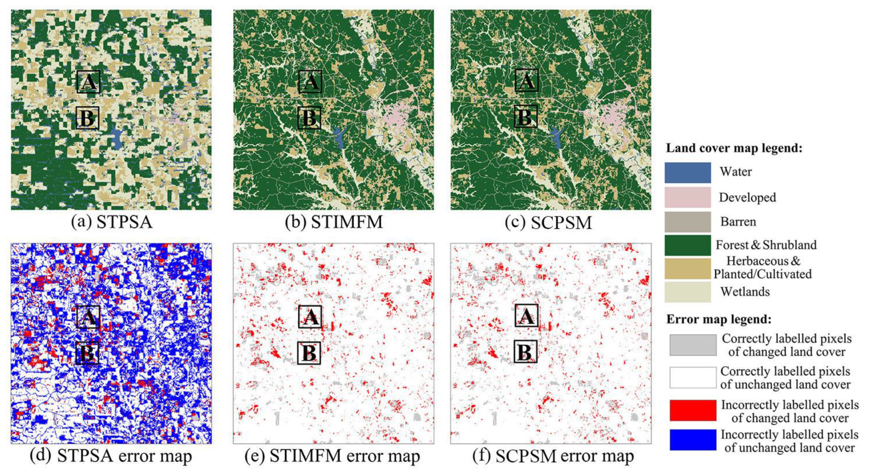
The predicted land cover maps from different methods are shown in Figure 6. The maps generated from STIMFM and SCPSM in Figure 6b,c were visually more similar to the reference map in Figure 3f than that generated from STPSA in Figure 6a. Many Forest & Shrubland pixels in green color in Figure 6a were incorrectly labeled as Wetlands pixels in the STPSA map. Many pixels incorrectly predicted as being of the unchanged class were found in the error map from STPSA, and were mostly eliminated in the error maps from STIMFM and SCPSM, showing that both STIMFM and SCPSM can predict unchanged pixels with better accuracy.

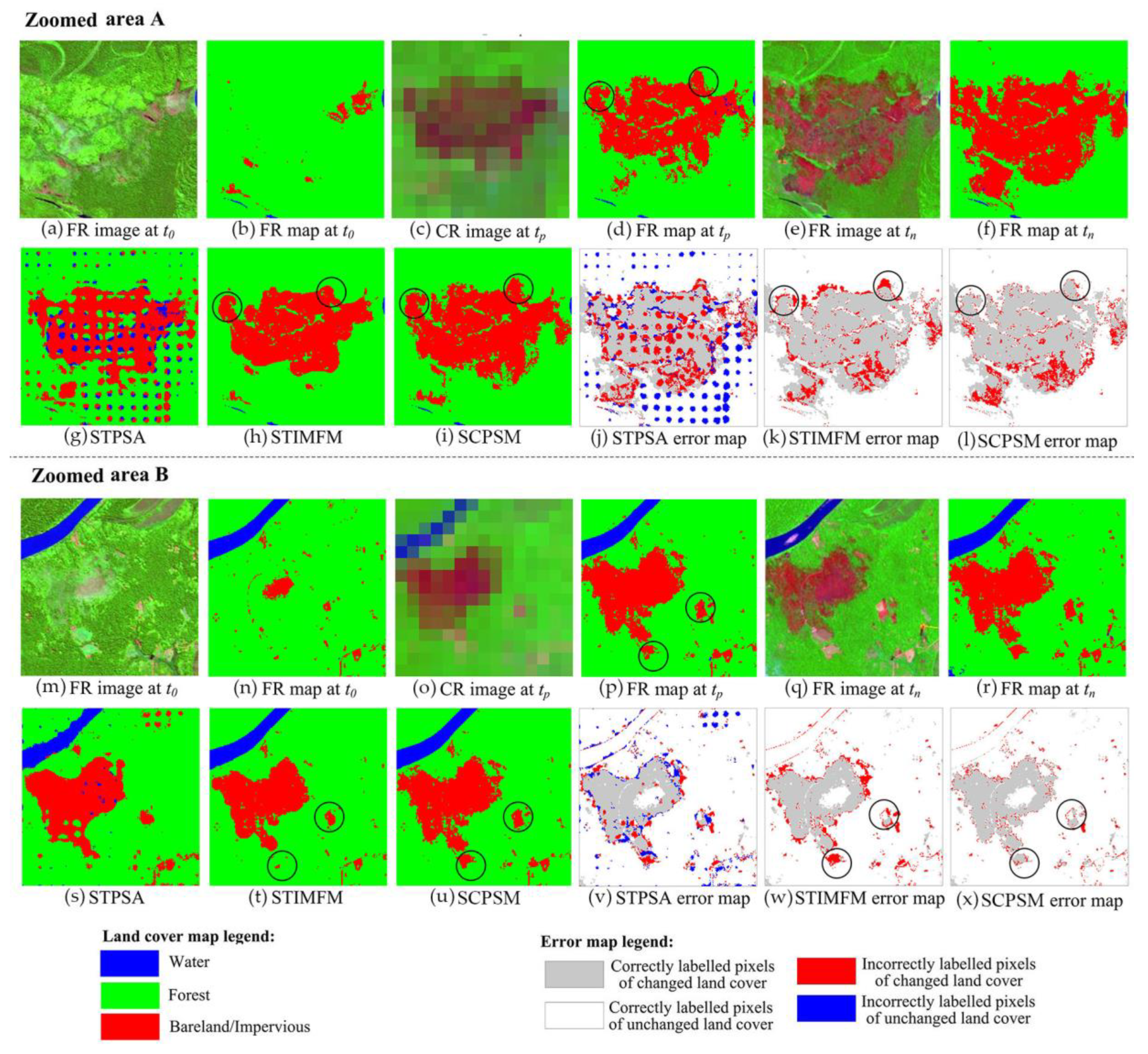
Figure 7 shows the zoomed areas in the outputs generated from the different methods. In both of the zoomed areas, the predicted map from STPSA was relatively dissimilar to the reference FR map at t_p in terms of the representation of spatial detail. For instance, in area A, the linear Developed class feature highlighted in the black ellipse was partly predicted by STPSA. However, since STPSA used the CR class fraction images unmixed from the CR remote sensing image at t_p as input and the analysis constrained to require that the class fractions should be unchanged between the input CR class fraction image and the output FR map, any errors in the class fraction images inevitably impact negatively on the map output from STPSA. In contrast, the linear Developed class feature was better predicted in the maps from STIMFM and SCPSM. In the zoomed area B, the predicted FR map from STIMFM contained rounded boundaries for the changed object highlighted in the black circles. This is because STIMFM uses the spatial dependence model from a spatially neighboring pixel in the spatial term, which is most suitable for objects that are larger than the size of the CR pixel that may over-smooth patch boundaries [5,34]. The boundaries between classes were better predicted in the map generated from SCPSM, showing that incorporating FR same-class pixels in STSPM can enhance the final map in terms of the spatial detail represented. In the error maps for the zoomed areas A and B, the map generated from STPSA contained many incorrectly labelled pixels. This is because these models are constrained to maintain the class fractions between the input CR class fraction image and the output FR map, and the predicted maps were affected by errors in the class fraction images. The incorrectly predicted unchanged pixels were not found in the maps from STIMFM and SCPSM, and the incorrectly predicted changed pixels were reduced in the map from SCPSM than that from STIMFM.

The accuracies of the predicted FR maps from different methods are shown in

Table 1. The error and accuracies (%) for changed pixels, unchanged pixels, and all pixels (overall accuracy) of different methods in the NLCD experiment.

			Mapping Method
			STPSA	STIMFM	SCPSM
Error	Omission error	Water	28.44	11.79	11.12
		Developed	82.61	0.00	0.00
		Barren	21.22	1.99	1.99
		Forest & Shrubland	50.02	2.62	2.05
		Herbaceous & Planted/Cultivated	27.37	16.63	15.58
		Wetlands	35.44	0.16	0.20
	Commission error	Water	87.33	2.32	2.46
		Developed	25.19	0.10	0.24
		Barren	90.70	10.98	11.91
		Forest & Shrubland	12.71	3.76	3.50
		Herbaceous & Planted/Cultivated	43.28	12.19	9.66
		Wetlands	75.47	0.71	0.62
Accuracy	Changed pixels		33.59	59.48	64.46
	Unchanged pixels		55.58	100.00	100.00
	Overall accuracy		53.26	95.72	96.25

. The STIMFM and SCPSM generated the lowest omission and commission errors for different classes. For the Forest & Shrubland classes and Herbaceous & Planted/Cultivated classes, which were the two dominant land cover classes in the reference map, SCPSM generated both the lowest omission and commission errors. For the Wetlands classes (the percentage was 13.05%), SCPSM generated relatively higher omission errors but lower commission errors than STIMFM. For changed pixels, the accuracy from STPSA was 33.59%, and the accuracy increased to 59.48% from STIMFM, and increased to 64.46% from SCPSM, showing that SCPSM can predict with the highest accuracy for changed pixels. The accuracy of the classifications of unchanged pixels increased from 55.58% from STPSA to 100% from both STIMFM and SCPSM. The prediction accuracies for unchanged pixels were higher than for changed pixels for all the STSPM methods. This is because the FR maps were used in these STSPM algorithms, and an FR pixel has a higher probability of being labelled with the class of that FR pixel in the input FR map than other classes, according to the temporal dependence model used in STSPM. SCPSM generated the highest overall accuracy, indicating its suitability for land cover mapping.

4.2. Forest Fire Experiment

In Figure 8, the predicted map from STPSA contained many small speckle-like artifacts. This is because the class fractions in the map produced from STPSA must be the same as those in the CR class fraction images input to the analysis, and the error in class fraction images resulted in the speckle-like artifacts. For instance, if a CR pixel contains 100% of Forest pixels but the unmixed class fraction images contain 5% of Bareland/Impervious class, then 16 × 16 × 5% = 13 FR pixels will be labelled as Bareland/Impervious class in the area represented by this CR pixel. The speckle-like artifacts were eliminated in the maps from STIMFM and SCPSM because they did not constrain the analysis to maintain the class fraction information. The FR maps from STIMFM and SCPSM were close to the reference map in Figure 4f. Most of the incorrectly labelled pixels of unchanged land cover in blue color in Figure 8e,f were eliminated in the STIMFM and SCPSM maps.

Figure 9 shows the zoomed areas which experienced forest fire in the period t₀ to t_n in the maps produced by the different methods. The map from STPSA contained many speckle-like artifacts which were eliminated in the maps from STIMFM and SCPSM. The spatial detail of the burned area in the map from STPSA was dissimilar to the reference FR map at t_p. The map from STIMFM contained rounded boundaries such as those highlighted in the black circles in zoomed area A, and parts of the burned area were not predicted in the map from STIMFM, highlighted in the black circles in zoomed area B. In contrast, the map from SCPSM was more similar to the reference map than that from STIMFM. The spatial details of the burned area were better reconstructed in the SCPSM map in zoomed area A, and most of the missing parts of the burned area in the STIMFM map highlighted in the black circles in zoomed area B were reconstructed in the SCPSM map. The error maps from STIMFM and SCPSM contained very few incorrectly labelled pixels, especially for unchanged classes. The maps from SCPSM contained the least error in both zoomed areas.

STIMFM and SCPSM generated the lowest omission and commission errors (

Table 2. The error and accuracies (%) for changed pixels, unchanged pixels and all pixels (overall accuracy) of different methods in the forest fire experiment.

			Mapping Method
			STPSA	STIMFM	SCPSM
Error	Omission error	Water	28.11	5.59	5.02
		Forest	8.63	1.02	1.45
		Bareland/Impervious	15.43	18.11	9.89
	Commission error	Water	15.75	2.71	2.29
		Forest	4.12	3.51	1.99
		Bareland/Impervious	37.57	6.87	8.84
Accuracy	Changed pixels		66.29	65.81	73.63
	Unchanged pixels		91.41	99.99	99.99
	Overall accuracy		88.59	96.15	97.03

). SCPSM generated the lowest omission and commission errors for the Water class. The transition from Forest to Bareland/Impervious due to forest fire is the dominant land cover change trajectory in this area. STIMFM generated lower omission error for the Forest class but a much higher omission error for the Bareland/Impervious class than SCPSM. For instance, many Bareland/Impervious pixels were not mapped in the result from STIMFM in Figure 9, showing that STIMFM underestimated the burned areas due to forest fire in this experiment. SCPSM generated the lowest commission error for Forest class, and STIMFM generated the lowest commission error for the Bareland/Impervious class. STIMFM generated the highest accuracy for changed pixels, and STIMFM and SCPSM generated the highest accuracy for unchanged pixels in Table 2. The overall accuracy increased from 88.59% for STPSA, and increased to 96.15% for STIMFM and 97.03% for SCPSM.

4.3. Forest Clearance Experiment

In Figure 10d, the error map from STPSA contained many pixels incorrectly labelled as changed and unchanged. A visual comparison shows that the error maps from STIMFM and SCPSM contained fewer incorrectly predicted unchanged pixels than that from STPSA. In both zoomed areas in Figure 11, the map from STPSA contained many speckle-like artifacts due to class fraction errors from spectral unmixing. In zoomed area A, the class boundary from SCPSM highlighted in the black circle was more similar to the reference map than that from STIMFM. In zoomed area B, the corners of the Non-forest patch from STIMFM were rounded due to over-smoothing, and the shape of corners was better mapped using SCPSM. In both zoomed areas, the error map from STPSA contained many incorrectly predicted changed and unchanged pixels. The error maps from STIMFM and SCPSM eliminated most of the incorrectly predicted unchanged pixels. The error map from SCPSM contained fewer incorrectly predicted changed pixels than that from STIMFM, such as those highlighted in the black circles in both zoomed areas.

SCPSM generated the fewest omission and commission errors for Forest class and the fewest commission error for Non-forest among all methods in

Table 3. The error and accuracies (%) for changed pixels, unchanged pixels and all pixels (overall accuracy) of different methods in the forest clearance experiment.

			Mapping Method
			STPSA	STIMFM	SCPSM
Error	Omission error	Forest	3.47	1.88	0.67
		Non-forest	13.03	5.82	5.87
	Commission error	Forest	7.75	3.56	3.55
		Non-forest	6.02	3.11	1.14
Accuracy	Changed pixels		83.24	82.99	86.66
	Unchanged pixels		95.26	100.00	99.99
	Overall accuracy		92.86	96.61	97.33

. SCPSM generated the highest accuracy for changed pixels, but the predicted accuracy for unchanged pixels was 0.01% lower than STIMFM. The overall accuracy was slightly lower than 93% for STPSA, and increased to 96.61% for STIMFM and 97.33% for SCPSM.

5. Discussion

The results show that SCPSM yielded FR land cover predictions with a high overall accuracy. Critically, it appears that SCPSM made fuller use of the FR data available, notably the information obtained from same-class pixels, in producing its predictions. Four key issues are apparent and explored further in this section; the difference in the usage between the FR maps and the FR images in STSPM is introduced, and the methods of identifying same-class pixels from the FR images are discussed. The difference in predicting the percentage of FR pixels of different classes from STPSA, STIMFM, and SCPSM is discussed. The performance of SCPSM is also related to the degree of land cover change in the study area and the model parameters, which are also discussed in the following sub-sections.

5.1. Differences in the Usage Between the FR Maps and the FR Images in STSPM

Compared with traditional STSPMs, which use FR maps that pre- and post-date the CR image, SCPSM also incorporated FR images as ancillary data. The FR maps and images played different roles in STPSM. In the use of FR maps, each pixel was assigned to one specific class in the maps. The error in labeling the FR pixels could evidently affect the use of FR maps in STSPM. In contrast, in the use of FR images, the identification of same-class pixels did not label the FR pixel to any land cover classes, and only computed the similarity between the FR pixel in the local window and the target FR pixel. SCPSM used the spatial distribution of same-class pixels within the local window to assist the prediction of FR land cover spatial distributions, and experiments showed that SCPSM can better predict the spatial details of changed land cover objects. The advantage was, for example, clear in the prediction of burned areas in the forest fire experiment and in predicting the spatial details of the non-forest patch in the forest clearance experiment.

5.2. Methods of Identifying Same-Class Pixels

The method identifying same-class pixels in SCPSM was based on the spectral distance between the target FR pixel and a neighboring FR pixel within a local window centered on the target FR pixel. The selection of same-class pixels was similar to the selection of spectrally similar pixels in the field of spatio-temporal reflectance image fusion (STIF) [26,35,36]. The effect of different same-class pixel selection methods according to different spectrally similar pixel selection schemes used in STIF could be explored in SCPSM in the future. For instance, the same-class pixels can be selected using a non-local searching approach, assuming same-class pixels can be located in different regions of the image [37,38].

5.3. Comparison of Different Methods in Predicting the Percentage of FR Pixels of Different Classes

The percentage of each class in the predicted maps was compared with that in the reference map in each experiment, and the corresponding differences are shown in Figure 12. First, among different methods and in all experiments, STPSA generated the largest absolute difference in the percentage of FR pixels for all classes and in all experiments. In particular, STPSA underestimated about $27\%\times 800\times 800=172800$ FR pixels of Forest & Shrubland class, and overestimated about $21\%\times 800\times 800=134400$ FR pixels of Wetlands class in the NLCD experiment. This was clear by comparing the STPSA map in Figure 6a with the reference map in Figure 3f, in which many Forest & Shrubland pixels were incorrectly labeled as Wetlands pixels from STPSA. Second, STIMFM and SCPSM over- or underestimated the FR pixel of each class simultaneously. For instance, in the forest fire experiment, both STIMFM and SCPSM overestimated the FR pixel number of Forest class, and they underestimated the FR pixel number of Water and Bareland/Impervious classes. The main reason was that STIMFM and SCPSM had the same spatial, temporal, and spectral terms in their objective functions. Third, STIMFM generated relatively smaller absolute differences than SCPSM for Forest & Shrubland and Herbaceous & Planted/Cultivated classes in the NLCD experiment, as well as Forest and Non-forest classes in the forest clearance experiment. However, STIMFM only decreased the absolute difference by less than 0.3%, compared with SCPSM for these classes. By contrast, SCPSM decreased the absolute difference by about 1.5% compared with STIMFM for Water and Forest classes in the forest fire experiment.

5.4. Influencing Factors

5.4.1. The Degree of Land Cover Change in the Study Area

The accuracies of predicting changed pixels and unchanged pixels were different for SCPSM. In all the three experiments, the accuracies from both STIMFM and SCPSM were close to 100% for unchanged pixels and 60–80% for changed pixels. This shows that it was more difficult to predict accurately for changed than for unchanged pixels. The reason was that if a pixel had an unchanged class in the FR maps at t₀ and t_n, it was more likely to have an unchanged class in the FR map at t_p. The temporal term used in STIMFM and SCPSM gave a higher probability of predicting an FR pixel as an unchanged class than changed class. If an FR pixel was changed, the uncertainty in predicting its label was much larger in STSPM. One way to increase the accuracy of SCPSM is to accurately detect the sub-pixel scale class change within the CR pixels. For instance, in the STSPM proposed by Li et al. [39], a class fraction change detection is first applied to the CR class fraction images at time t₀ and t_p. Then the prediction of an FR pixel label (assuming its label is c) is related to the cth CR fraction change detection result in the corresponding CR pixel; the pixel’s label is assumed unchanged in STSPM if the cth class fraction in the corresponding CR pixel is detected as unchanged, and the pixel’s label is updated by STSPM if the cth class fraction in the corresponding CR pixel is detected as changed. In this way the STSPM is simplified to only predict the changed FR pixel labels, and the temporal term may not have a negative effect in this case. However, the linear mixture model is used in [39] to produce the CR fraction images, and the accuracy of class fraction image accuracy would decrease with low inter-class spectral separability. Considering that spectral unmixing is an open problem, future studies on class fraction extraction and sub-pixel change detection and their applications in SCPSM should be developed.

5.4.2. Model Parameters

The performance of SCPSM was influenced by the weights used in the analysis. The optimal weights can be selected based on criteria such as inter-class spectral separability, which could be used to balance the spectral and spatial terms [40], and based on the spatial heterogeneity of the CR class fraction images, which could be used to give different weights of spatial terms to different CR pixels [41]. In real applications in which subsets of training data are usually available, the optimal weights can also be defined based on the subsets of training samples.

6. Conclusions

A novel STSPM which uses same-class FR neighborhood pixels extracted from the ancillary FR remote sensing images was proposed in this paper. In addition to the FR land cover maps at the times that pre- and post-date the CR image at the prediction time, the proposed SCPSM inputs FR remote sensing images to constrain the analysis. The same-class FR neighborhood pixels selected from the FR images are used to model the spatial distribution for FR pixels, based on the assumption that spectrally similar pixels are more likely to belong to the same class. This paper is, to the best of our knowledge, the first to report on the use of same-class pixels extracted from the ancillary FR images in STSPM.

The proposed SCPSM has two advantages against the state-of-the-art STSPM algorithms, including STPSA and STIMFM. First, SCPSM could increase the overall accuracy compared with STPSA and STIMFM in this paper. Since the overall accuracy is a key metric in assessing the accuracy of land cover maps, SCPSM is effective in producing land cover maps due to its higher overall accuracy. Second, SCPSM could also predict the pixels of changed pixels more accurately than both STPSA and STIMFM. The detection and mapping of land cover change are important issues in the society of remote sensing, and these tasks are especially difficult when the change occurs at the sub-pixel scale. SCPSM is superior to STPSA and STIMFM in monitoring the substantial sub-pixel scale spatio-temporal change of surface land covers. Finally, SCPSM better predicted the spatial details of land cover spatial patterns. Since SCPSM adopted the same-class pixels extracted from FR images to indicate detailed land cover spatial distribution information within the CR pixels, it could avoid producing over-smoothed boundaries between land cover patches that result from STSPM algorithms, which only use the spatial dependence model to model the land cover spatial distribution. Thus, SCPSM is more suitable in land cover mapping, especially in fragmented landscapes, than the other STSPMs.

Although SCPSM has numerous advantages over the comparison algorithms, it has limitations and faces challenges in several aspects. First, SCPSM is superior to STPSA in the accuracy of predicting unchanged FR pixel labels, but it may generate a slightly lower accuracy than STIMFM, such as in the forest clearance experiment. This is because, although SCPSM and STIMFM have the same spatial, spectral, and temporal terms, SCPSM has an additional ancillary data term. In SCPSM, if an FR is unchanged and the labels between the same-class FR pixels at t_p and the temporal neighborhood FR pixels at t₀ and t_p are different, the ancillary data term in SCPSM makes the target FR pixel have a changed FR pixel label, and this effect may decrease the accuracy in predicting unchanged FR pixel labels in SCPSM. Second, SCPSM uses more data, i.e., the FR images that pre- and post-date the prediction time, as input in comparison with STIMFM, and uses a relative longer time than STIMFM in computation. Lastly, SCPSM has limitations in predicting the labels of changed pixels, regardless of the fact that it predicts higher accuracy of changed pixels than STPSA and STIMFM. SCPSM predicted the labels accurately for more than 99.99% of unchanged FR pixels in all the experiments, but it predicted labels accurately for only 64.46%–86.66% of changed FR pixels. Means to enhance the method, such as using an advanced method to accurately detect the sub-pixel scale class change within the CR pixels, and the potential of different methods for the selection of same-class pixels should be explored further for the study of mapping spatio-temporal changes of land use and land covers.

References

- Chapin, F.S.; Zavaleta, E.S.; Eviner, V.T.; Naylor, R.L.; Vitousek, P.M.; Reynolds, H.L.; Hooper, D.U.; Lavorel, S.; Sala, O.E.; Hobbie, S.E.; et al. Consequences of changing biodiversity. Nature 2000, 405, 234–242. [Google Scholar] [CrossRef] [PubMed]
- Foley, J.A.; DeFries, R.; Asner, G.P.; Barford, C.; Bonan, G.; Carpenter, S.R.; Chapin, F.S.; Coe, M.T.; Daily, G.C.; Gibbs, H.K.; et al. Global consequences of land use. Science 2005, 309, 570–574. [Google Scholar] [CrossRef] [PubMed]
- Hsieh, P.F.; Lee, L.C.; Chen, N.Y. Effect of spatial resolution on classification errors of pure and mixed pixels in remote sensing. IEEE Trans. Geosci. Remote Sens. 2001, 39, 2657–2663. [Google Scholar] [CrossRef]
- Keshava, N.; Mustard, J.F. Spectral unmixing. IEEE Signal Process. Mag. 2002, 19, 44–57. [Google Scholar] [CrossRef]
- Atkinson, P.M. Issues of uncertainty in super-resolution mapping and their implications for the design of an inter-comparison study. Int. J. Remote Sens. 2009, 30, 5293–5308. [Google Scholar] [CrossRef]
- Foody, G.M.; Muslim, A.M.; Atkinson, P.M. Super-resolution mapping of the waterline from remotely sensed data. Int. J. Remote Sens. 2005, 26, 5381–5392. [Google Scholar] [CrossRef]
- Jia, Y.; Ge, Y.; Chen, Y.; Li, S.; Heuvelink, G.B.M.; Ling, F. Super-resolution land cover mapping based on the Convolutional Neural Network. Remote Sens. 2019, 11, 1815. [Google Scholar] [CrossRef]
- Wang, X.; Ling, F.; Yao, H.; Liu, Y.; Xu, S. Unsupervised sub-pixel water body mapping with Sentinel-3 OLCI image. Remote Sens. 2019, 11, 327. [Google Scholar] [CrossRef]
- Xu, X.; Tong, X.; Plaza, A.; Zhong, Y.; Xie, H.; Zhang, L. Joint sparse sub-pixel mapping model with endmember variability for remotely sensed imagery. Remote Sens. 2017, 9, 15. [Google Scholar] [CrossRef]
- Kasetkasem, T.; Arora, M.K.; Varshney, P.K. Super-resolution land cover mapping using a Markov random field based approach. Remote Sens. Environ. 2005, 96, 302–314. [Google Scholar] [CrossRef]
- Ling, F.; Boyd, D.; Ge, Y.; Foody, G.M.; Li, X.; Wang, L.; Zhang, Y.; Shi, L.; Shang, C.; Li, X.; et al. Measuring River Wetted Width From Remotely Sensed Imagery at the Subpixel Scale With a Deep Convolutional Neural Network. Water Resour. Res. 2019, 55, 5631–5649. [Google Scholar] [CrossRef]
- Li, X.; Li, X.; Foody, G.; Yang, X.; Zhang, Y.; Du, Y.; Ling, F. Optimal Endmember-Based Super-Resolution Land Cover Mapping. IEEE Geosci. Remote Sens. Lett. 2019, 16, 1279–1283. [Google Scholar] [CrossRef]
- Li, X.; Ling, F.; Foody, G.M.; Ge, Y.; Zhang, Y.; Du, Y. Generating a series of fine spatial and temporal resolution land cover maps by fusing coarse spatial resolution remotely sensed images and fine spatial resolution land cover maps. Remote Sens. Environ. 2017, 196, 293–311. [Google Scholar] [CrossRef]
- Wang, Q.; Shi, W.; Atkinson, P.M. Spatiotemporal subpixel mapping of time-series images. IEEE Trans. Geosci. Remote Sens. 2016, 54, 5397–5411. [Google Scholar] [CrossRef]
- Ling, F.; Li, W.; Du, Y.; Li, X. Land cover change mapping at the subpixel scale with different spatial-resolution remotely sensed imagery. IEEE Geosci. Remote Sens. Lett. 2011, 8, 182–186. [Google Scholar] [CrossRef]
- He, D.; Zhong, Y.; Feng, R.; Zhang, L. Satial-temporal sub-pixel mapping based on swarm intelligence theory. Remote Sens. 2016, 8, 894. [Google Scholar] [CrossRef]
- Li, X.; Ling, F.; Du, Y.; Feng, Q.; Zhang, Y. A spatial-temporal Hopfield neural network approach for super-resolution land cover mapping with multi-temporal different resolution remotely sensed images. ISPRS J. Photogramm. Remote Sens. 2014, 93, 76–87. [Google Scholar] [CrossRef]
- Wang, Q.; Shi, W.; Atkinson, P.M.; Li, Z. Land cover change detection at subpixel resolution with a Hopfield neural network. IEEE J. Sel. Top. Appl. Earth Obs. Remote Sens. 2015, 8, 1339–1352. [Google Scholar] [CrossRef]
- Wu, K.; Du, Q.; Wang, Y.; Yang, Y. Supervised sub-pixel mapping for change detection from remotely sensed images with different resolutions. Remote Sens. 2017, 9, 284. [Google Scholar] [CrossRef]
- Yang, X.; Xie, Z.; Ling, F.; Li, X.; Zhang, Y.; Zhong, M. Spatio-temporal super-resolution land cover mapping based on fuzzy C-means clustering. Remote Sens. 2018, 10, 1212. [Google Scholar] [CrossRef]
- Zhang, Y.; Ling, F.; Foody, G.M.; Ge, Y.; Boyd, D.S.; Li, X.; Du, Y.; Atkinson, P.M. Mapping annual forest cover by fusing PALSAR/PALSAR-2 and MODIS NDVI during 2007-2016. Remote Sens. Environ. 2019, 224, 74–91. [Google Scholar] [CrossRef]
- Atkinson, P.M. Sub-pixel target mapping from soft-classified, remotely sensed imagery. Photogramm. Eng. Remote Sens. 2005, 71, 839–846. [Google Scholar] [CrossRef]
- Ling, F.; Xiao, F.; Du, Y.; Xue, H.P.; Ren, X.Y. Waterline mapping at the subpixel scale from remote sensing imagery with high-resolution digital elevation models. Int. J. Remote Sens. 2008, 29, 1809–1815. [Google Scholar] [CrossRef]
- Aplin, P.; Atkinson, P.M. Sub-pixel land cover mapping for per-field classification. Int. J. Remote Sens. 2001, 22, 2853–2858. [Google Scholar] [CrossRef]
- Chen, Y.; Ge, Y.; An, R.; Chen, Y. Super-resolution mapping of impervious surfaces from remotely sensed imagery with Points-of-Interest. Remote Sens. 2018, 10, 242. [Google Scholar] [CrossRef]
- Gao, F.; Masek, J.; Schwaller, M.; Hall, F. On the blending of the Landsat and MODIS surface reflectance: Predicting daily Landsat surface reflectance. IEEE Trans. Geosci. Remote Sens. 2006, 44, 2207–2218. [Google Scholar] [CrossRef]
- Zhu, X.; Chen, J.; Gao, F.; Chen, X.; Masek, J.G. An enhanced spatial and temporal adaptive reflectance fusion model for complex heterogeneous regions. Remote Sens. Environ. 2010, 114, 2610–2623. [Google Scholar] [CrossRef]
- Zhu, X.; Helmer, E.H.; Gao, F.; Liu, D.; Chen, J.; Lefsky, M.A. A flexible spatiotemporal method for fusing satellite images with different resolutions. Remote Sens. Environ. 2016, 172, 165–177. [Google Scholar] [CrossRef]
- Ling, F.; Du, Y.; Xiao, F.; Li, X.D. Subpixel Land Cover Mapping by Integrating Spectral and Spatial Information of Remotely Sensed Imagery. IEEE Geosci. Remote Sens. Lett. 2012, 9, 408–412. [Google Scholar] [CrossRef]
- Wu, K.; Zhong, Y.; Wang, X.; Sun, W. A Novel Approach to Subpixel Land-Cover Change Detection Based on a Supervised Back-Propagation Neural Network for Remotely Sensed Images With Different Resolutions. IEEE Geosci. Remote Sens. Lett. 2017, 14, 1750–1754. [Google Scholar] [CrossRef]
- Kavzoglu, T.; Colkesen, I. A kernel functions analysis for support vector machines for land cover classification. Int. J. Appl. Earth Obs. Geoinf. 2009, 11, 352–359. [Google Scholar] [CrossRef]
- Xu, Y.; Huang, B. A spatio-temporal pixel-swapping algorithm for subpixel land cover mapping. IEEE Geosci. Remote Sens. Lett. 2014, 11, 474–478. [Google Scholar] [CrossRef]
- Ardila, J.P.; Tolpekin, V.A.; Bijker, W.; Stein, A. Markov-random-field-based super-resolution mapping for identification of urban trees in VHR images. ISPRS J. Photogramm. Remote Sens. 2011, 66, 762–775. [Google Scholar] [CrossRef]
- Tatem, A.J.; Lewis, H.G.; Atkinson, P.M.; Nixon, M.S. Super-resolution land cover pattern prediction using a Hopfield neural network. Remote Sens. Environ. 2002, 79, 1–14. [Google Scholar] [CrossRef]
- Ma, J.; Zhang, W.; Marinoni, A.; Gao, L.; Zhang, B. Performance assessment of ESTARFM with different similar-pixel identification schemes. J. Appl. Remote Sens. 2018, 12, 025017. [Google Scholar] [CrossRef]
- Zhu, X.; Cai, F.; Tian, J.; Williams, T.K.-A. Spatiotemporal fusion of multisource remote sensing data: Literature survey, taxonomy, principles, applications, and future directions. Remote Sens. 2018, 10, 527. [Google Scholar] [CrossRef]
- Cheng, Q.; Liu, H.; Shen, H.; Wu, P.; Zhang, L. A spatial and temporal nonlocal filter-based data fusion method. IEEE Trans. Geosci. Remote Sens. 2017, 55, 4476–4488. [Google Scholar] [CrossRef]
- Zhao, Y.; Huang, B.; Song, H. A robust adaptive spatial and temporal image fusion model for complex land surface changes. Remote Sens. Environ. 2018, 208, 42–62. [Google Scholar] [CrossRef]
- Li, X.; Du, Y.; Ling, F. Sub-pixel-scale land cover map updating by integrating change detection and sub-pixel mapping. Photogramm. Eng. Remote Sens. 2015, 81, 59–67. [Google Scholar] [CrossRef]
- Tolpekin, V.A.; Stein, A. Quantification of the effects of land-cover-class spectral separability on the accuracy of Markov-random-field-based superresolution mapping. IEEE Trans. Geosci. Remote Sens. 2009, 47, 3283–3297. [Google Scholar] [CrossRef]
- Li, X.; Du, Y.; Ling, F. Spatially adaptive smoothing parameter selection for Markov random field based sub-pixel mapping of remotely sensed images. Int. J. Remote Sens. 2012, 33, 7886–7901. [Google Scholar] [CrossRef]
Figure 1.
The flowchart of same-class pixels-based STSPM model (SCPSM).
Figure 2.
The schematic diagram of spatially neighboring pixels in the spatial term and same-class pixels in the ancillary data term. (
a) Spatially neighboring fine spatial resolution (FR) pixels in the spatial term. (
b) Same-class FR pixels selected from FR image at
t0 in the ancillary data term; (
c) same-class FR pixels selected from FR image at
tn in the ancillary data term; (
d) final same-class FR pixels used in the ancillary data term. The FR pixels as same-class pixels from images at
t0 and
tn in (
b,
c) are randomly selected in
Figure 3.
The fine spatial resolution (FR) images, coarse spatial resolution (CR) image, FR land cover maps and FR land cover change map used in the National Land Cover Database (NLCD) experiment. The scale factor s was 16. (a) FR image at t0 from Landsat image acquired on 7 October 2011; (b) FR image at tp from Landsat image acquired on 13 November 2013; (c) FR image at tn from Landsat image acquired on 5 November 2016; (d) CR image at tp resampled from (b); (e) FR land cover map at t0; (f) FR land cover map at tp (reference land cover map); (g) FR image at tn; (h) FR land cover change map that was produced by comparing (e–g).
Figure 4.
The FR images, CR image, FR land cover maps and FR land cover change map used in the experiment for the forest fire experiment. The scale factor s was 16. (a) FR image at t0 from Landsat image acquired on 7 June 2010; (b) FR image at tp from Landsat image acquired on 11 September 2010; (c) FR image at tn from Landsat image acquired on 27 September 2010; (d) CR image at tp resampled from (b); (e) FR land cover map at t0; (f) FR land cover map at tp (reference land cover map); (g) FR image at tn; (h) FR land cover change map that was produced by comparing (e–g).
Figure 5.
The FR images, CR image, FR land cover maps, and FR land cover change map used in the forest clearance experiment. The scale factor s was 16. (a) FR image at t0 from Landsat image acquired on 23 July 2001; (b) FR image at tp from Landsat image acquired on 21 July 2003; (c) FR image at tn from Landsat image acquired on 5 June 2004; (d) CR image at tp from MODIS image acquired on 21 July 2003; (e) FR land cover map at t0; (f) FR land cover map at tp (reference land cover map); (g) FR image at tn; (h) FR land cover change map that was produced by comparing (e–g).
Figure 6.
The result of land cover maps predicted from different methods, and the corresponding error maps in the NLCD experiment. (a) spatio-temporal PSA-based SPM (STPSA); (b) spatio-temporal image and map fusion model (STIMFM); (c) same-class pixels-based STSPM model (SCPSM); (d) STPSA error map; (e) STIMFM error map; (f) SCPSM error map.
Figure 7.
Input, reference, resulting land cover maps and error maps for the zoomed areas in
Figure 6 in the NLCD experiment. Each zoomed area contains 80 × 80 FR pixels. (
a–
l) are the input, reference, resulting maps and error maps for zoomed area A: (
a) FR image at
t0; (
b) FR map at
c) CR image at
tp; (
d) FR map at
e) FR image at
tn; (
f) FR map at
g) STPSA; (
h) STIMFM; (
i) SCPSM; (
j) STPSA error map; (
k) STIMFM error map; (
l) SCPSM error map. (
m–
x) are the input, reference, resulting maps and error maps for zoomed area B: (
m) FR image at
n) FR map at
o) CR image at
p) FR map at
q) FR image at
r) FR map at
s) STPSA; (
t) STIMFM; (
u) SCPSM; (
v) STPSA error map; (
w) STIMFM error map; (
x) SCPSM error map.
Figure 8.
The result of land cover maps predicted from different methods and the corresponding error maps in the experiment for the forest fire experiment. (a) STPSA; (b) STIMFM; (c) SCPSM; (d) STPSA error map; (e) STIMFM error map; (f) SCPSM error map.
Figure 9.
Input, reference, resulting land cover maps, and error maps for the zoomed areas in
Figure 8 in the forest fire experiment. Each zoomed area contains 240 × 240 FR pixels. (
a)–(
m)–(
Figure 10.
The land cover maps predicted from different methods and the corresponding error maps in the forest clearance experiment. (a) STPSA; (b) STIMFM; (c) SCPSM; (d) STPSA error map; (e) STIMFM error map; (f) SCPSM error map.
Figure 11.
Figure 10 in the forest clearance experiment. Each zoomed area contains 192 × 192 FR pixels. (
Figure 12.
The absolute differences between the percentage of FR pixels of each class in the predicted and reference maps in the three experiments. Positive value means the predicted number of pixels is higher than that in the reference map for a class, and negative value means the predicted number of pixels is lower than that in the reference map for a class.